Fundamentals of structural dynamics
Bạn đang xem bản rút gọn của tài liệu. Xem và tải ngay bản đầy đủ của tài liệu tại đây (23.48 MB, 217 trang )
Course “Fundamentals of Structural Dynamics”
An-Najah National University
April 19 - April 23, 2013
Lecturer: Dr. Alessandro Dazio, UME School
Course “Fundamentals of Structural Dynamics”
April 19 - April 23, 2013
4 Schedule of classes
Date
Fundamentals of Structural Dynamics
Day 1
Fri. April 19
2013
1 Course description
Aim of the course is that students develop a “feeling for dynamic problems” and acquire the theoretical
background and the tools to understand and to solve important problems relevant to the linear and, in
part, to the nonlinear dynamic behaviour of structures, especially under seismic excitation.
The course will start with the analysis of single-degree-of-freedom (SDoF) systems by discussing: (i)
Modelling, (ii) equations of motion, (iii) free vibrations with and without damping, (iv) harmonic, periodic and short excitations, (v) Fourier series, (vi) impacts, (vii) linear and nonlinear time history analysis, and (viii) elastic and inelastic response spectra.
Afterwards, multi-degree-of-freedom (MDoF) systems will be considered and the following topics will
be discussed: (i) Equation of motion, (ii) free vibrations, (iii) modal analysis, (iv) damping, (v) Rayleigh’s
quotient, and (vi) seismic behaviour through response spectrum method and time history analysis.
To supplement the suggested reading, handouts with class notes and calculation spreadsheets with selected analysis cases to self-training purposes will be distributed.
Lecturer:
Dr. Alessandro Dazio, UME School
Day 2
Sat. April 20
2013
Day 3
Sun. April 21
2013
Day 4
Mon. April 22
2013
2 Suggested reading
Time
Topic
09:00 - 10:30
1. Introduction
2. SDoF systems: Equation of motion and modelling
11:00 - 12:30
3. Free vibrations
14:30 - 16:00
Assignment 1
16:30 - 18:00
Assignment 1
9:00 - 10:30
4. Harmonic excitation
11:00 - 12:30
5. Transfer functions
14:30 - 16:00
6. Forced vibrations (Part 1)
16:30 - 18:00
6. Forced vibrations (Part 2)
09:00 - 10:30
7. Seismic excitation (Part 1)
11:00 - 12:30
7. Seismic excitation (Part 2)
14:30 - 16:00
Assignment 2
16:30 - 18:00
Assignment 2
9:00 - 10:30
8. MDoF systems: Equation of motion
11:00 - 12:30
9. Free vibrations
14:30 - 16:00
10. Damping
11. Forced vibrations
[Cho11]
Chopra A., “Dynamics of Structures”, Prentice Hall, Fourth Edition, 2011.
16:30 - 18:00
11. Forced vibrations
[CP03]
Clough R., Penzien J., “Dynamics of Structures”, Second Edition (revised), Computer and
Structures Inc., 2003.
09:00 - 10:30
12. Seismic excitation (Part 1)
[Hum12] Humar J.L., “Dynamics of Structures”. Third Edition. CRC Press, 2012.
3 Software
Day 5
Tue. April 23
2013
11:00 - 12:30
12. Seismic excitation (Part 2)
14:30 - 16:00
Assignment 3
16:30 - 18:00
Assignment 3
In the framework of the course the following software will be used by the lecturer to solve selected examples:
[Map10]
Maplesoft: “Maple 14”. User Manual. 2010
[Mic07]
Microsoft: “Excel 2007”. User Manual. 2007
[VN12]
Visual Numerics: “PV Wave”. User Manual. 2012
As an alternative to [VN12] and [Map10] it is recommended that students make use of the following
software, or a previous version thereof, to deal with coursework:
[Mat12]
MathWorks: “MATLAB 2012”. User Manual. 2012
A. Dazio, April 19, 2013
Page 1/2
Page 2/2
Course “Fundamentals of Structural Dynamics”
An-Najah 2013
Table of Contents
Course “Fundamentals of Structural Dynamics”
An-Najah 2013
3.2 Damped free vibrations ....................................................................... 3-6
Table of Contents...................................................................... i
3.2.1
Formulation 3: Exponential Functions ....................................................... 3-6
3.2.2
Formulation 1: Amplitude and phase angle............................................. 3-10
3.3 The logarithmic decrement .............................................................. 3-12
3.4 Friction damping ............................................................................... 3-15
1 Introduction
1.1 Goals of the course .............................................................................. 1-1
1.2 Limitations of the course..................................................................... 1-1
1.3 Topics of the course ............................................................................ 1-2
1.4 References ............................................................................................ 1-3
4 Response to Harmonic Excitation
4.1 Undamped harmonic vibrations ......................................................... 4-3
4.1.1
Interpretation as a beat ................................................................................ 4-5
4.1.2
Resonant excitation (ω = ωn) ....................................................................... 4-8
4.2 Damped harmonic vibration .............................................................. 4-10
4.2.1
2 Single Degree of Freedom Systems
2.1 Formulation of the equation of motion............................................... 2-1
2.1.1
Direct formulation......................................................................................... 2-1
2.1.2
Principle of virtual work............................................................................... 2-3
2.1.3
Energy Formulation...................................................................................... 2-3
2.2 Example “Inverted Pendulum”............................................................ 2-4
2.3 Modelling............................................................................................. 2-10
2.3.1
Structures with concentrated mass.......................................................... 2-10
2.3.2
Structures with distributed mass ............................................................. 2-11
2.3.3
Damping ...................................................................................................... 2-20
3 Free Vibrations
Resonant excitation (ω = ωn) ..................................................................... 4-13
5 Transfer Functions
5.1 Force excitation .................................................................................... 5-1
5.1.1
Comments on the amplification factor V.................................................... 5-4
5.1.2
Steady-state displacement quantities ........................................................ 5-8
5.1.3
Derivating properties of SDoF systems from harmonic vibrations....... 5-10
5.2 Force transmission (vibration isolation) ......................................... 5-12
5.3 Base excitation (vibration isolation)................................................. 5-15
5.3.1
Displacement excitation ........................................................................... 5-15
5.3.2
Acceleration excitation ............................................................................. 5-17
5.3.3
Example transmissibility by base excitation .......................................... 5-20
5.4 Summary Transfer Functions ........................................................... 5-26
3.1 Undamped free vibrations ................................................................... 3-1
3.1.1
Formulation 1: Amplitude and phase angle............................................... 3-1
3.1.2
Formulation 2: Trigonometric functions .................................................... 3-3
3.1.3
Formulation 3: Exponential Functions ....................................................... 3-4
6 Forced Vibrations
6.1 Periodic excitation .............................................................................. 6-1
6.1.1
Table of Contents
Page i
Steady state response due to periodic excitation..................................... 6-4
Table of Contents
Page ii
Course “Fundamentals of Structural Dynamics”
An-Najah 2013
Course “Fundamentals of Structural Dynamics”
An-Najah 2013
7.5 Elastic response spectra ................................................................... 7-42
6.1.2
Half-sine ........................................................................................................ 6-5
6.1.3
Example: “Jumping on a reinforced concrete beam”............................... 6-7
7.5.1
Computation of response spectra ............................................................ 7-42
6.2 Short excitation .................................................................................. 6-12
7.5.2
Pseudo response quantities...................................................................... 7-45
Step force .................................................................................................... 6-12
7.5.3
Properties of linear response spectra ..................................................... 7-49
6.2.2
Rectangular pulse force excitation .......................................................... 6-14
7.5.4
Newmark’s elastic design spectra ([Cho11]) ........................................... 7-50
6.2.3
Example “blast action” .............................................................................. 6-21
7.5.5
Elastic design spectra in ADRS-format (e.g. [Faj99])
(Acceleration-Displacement-Response Spectra) .................................... 7-56
6.2.1
7.6 Strength and Ductility ........................................................................ 7-58
7 Seismic Excitation
7.6.1
Illustrative example .................................................................................... 7-58
7.1 Introduction .......................................................................................... 7-1
7.6.2
“Seismic behaviour equation” .................................................................. 7-61
7.2 Time-history analysis of linear SDoF systems ................................. 7-3
7.6.3
Inelastic behaviour of a RC wall during an earthquake ........................ 7-63
Newmark’s method (see [New59]) .............................................................. 7-4
7.6.4
Static-cyclic behaviour of a RC wall ........................................................ 7-64
7.2.2
Implementation of Newmark’s integration scheme within
the Excel-Table “SDOF_TH.xls”.................................................................. 7-8
7.6.5
General definition of ductility ................................................................... 7-66
7.6.6
Types of ductilities .................................................................................... 7-67
7.2.3
Alternative formulation of Newmark’s Method. ....................................... 7-10
7.2.1
7.3 Time-history analysis of nonlinear SDoF systems ......................... 7-12
7.7 Inelastic response spectra ............................................................... 7-68
7.7.1
Inelastic design spectra............................................................................. 7-71
7.7.2
Determining the response of an inelastic SDOF system
by means of inelastic design spectra in ADRS-format ........................... 7-80
7.3.1
Equation of motion of nonlinear SDoF systems ..................................... 7-13
7.3.2
Hysteretic rules........................................................................................... 7-14
7.3.3
Newmark’s method for inelastic systems ................................................ 7-18
7.7.3
Inelastic design spectra: An important note............................................ 7-87
7.3.4
Example 1: One-storey, one-bay frame ................................................... 7-19
7.7.4
Behaviour factor q according to SIA 261 ................................................. 7-88
7.3.5
Example 2: A 3-storey RC wall .................................................................. 7-23
7.4 Solution algorithms for nonlinear analysis problems .................... 7-26
7.4.1
General equilibrium condition................................................................. 7-26
7.4.2
Nonlinear static analysis ........................................................................... 7-26
7.4.3
The Newton-Raphson Algorithm............................................................... 7-28
7.4.4
Nonlinear dynamic analyses ..................................................................... 7-35
7.4.5
Comments on the solution algorithms for
nonlinear analysis problems ..................................................................... 7-38
7.4.6
Simplified iteration procedure for SDoF systems with
idealised rule-based force-deformation relationships............................ 7-41
Table of Contents
Page iii
7.8 Linear equivalent SDOF system (SDOFe) ....................................... 7-89
7.8.1
Elastic design spectra for high damping values ..................................... 7-99
7.8.2
Determining the response of inelastic SDOF systems
by means of a linear equivalent SDOF system and
elastic design spectra with high damping ............................................. 7-103
7.9 References ........................................................................................ 7-108
8 Multi Degree of Freedom Systems
8.1 Formulation of the equation of motion............................................... 8-1
8.1.1
Equilibrium formulation ............................................................................... 8-1
8.1.2
Stiffness formulation ................................................................................... 8-2
Table of Contents
Page iv
Course “Fundamentals of Structural Dynamics”
An-Najah 2013
Course “Fundamentals of Structural Dynamics”
An-Najah 2013
8.1.3
Flexibility formulation ................................................................................. 8-3
10.3Classical damping matrices .............................................................. 10-5
8.1.4
Principle of virtual work............................................................................... 8-5
10.3.1 Mass proportional damping (MpD) ......................................................... 10-5
8.1.5
Energie formulation...................................................................................... 8-5
10.3.2 Stiffness proportional damping (SpD) .................................................... 10-5
8.1.6
“Direct Stiffness Method”............................................................................ 8-6
10.3.3 Rayleigh damping..................................................................................... 10-6
8.1.7
Change of degrees of freedom.................................................................. 8-11
10.3.4 Example....................................................................................................... 10-7
8.1.8
Systems incorporating rigid elements with distributed mass ............... 8-14
11 Forced Vibrations
9 Free Vibrations
11.1Forced vibrations without damping ................................................. 11-1
9.1 Natural vibrations ................................................................................. 9-1
11.1.1 Introduction ................................................................................................ 11-1
9.2 Example: 2-DoF system ...................................................................... 9-4
11.1.2 Example 1: 2-DoF system.......................................................................... 11-3
9.2.1
Eigenvalues ................................................................................................ 9-4
11.1.3 Example 2: RC beam with Tuned Mass Damper (TMD) without damping...
11-7
9.2.2
Fundamental mode of vibration .................................................................. 9-5
9.2.3
Higher modes of vibration ........................................................................... 9-7
11.2Forced vibrations with damping ..................................................... 11-13
9.2.4
Free vibrations of the 2-DoF system .......................................................... 9-8
11.2.1 Introduction .............................................................................................. 11-13
9.3 Modal matrix and Spectral matrix ..................................................... 9-12
11.3Modal analysis: A summary ............................................................ 11-15
9.4 Properties of the eigenvectors.......................................................... 9-13
12 Seismic Excitation
9.4.1
Orthogonality of eigenvectors .................................................................. 9-13
9.4.2
Linear independence of the eigenvectors................................................ 9-16
12.1Equation of motion............................................................................. 12-1
9.5 Decoupling of the equation of motion.............................................. 9-17
12.1.1 Introduction................................................................................................. 12-1
9.6 Free vibration response..................................................................... 9-22
9.6.1
Systems without damping ......................................................................... 9-22
9.6.2
Classically damped systems..................................................................... 9-24
12.1.2 Synchronous Ground motion.................................................................... 12-3
12.1.3 Multiple support ground motion ............................................................... 12-8
12.2Time-history of the response of elastic systems .......................... 12-18
12.3Response spectrum method ........................................................... 12-23
10 Damping
12.3.1 Definition and characteristics ................................................................. 12-23
10.1Free vibrations with damping ........................................................... 10-1
10.2Example .............................................................................................. 10-2
10.2.1 Non-classical damping ............................................................................ 10-3
10.2.2 Classical damping .................................................................................... 10-4
Table of Contents
Page v
12.3.2 Step-by-step procedure ......................................................................... 12-27
12.4Practical application of the response spectrum method
to a 2-DoF system ............................................................................ 12-29
12.4.1 Dynamic properties ................................................................................. 12-29
12.4.2 Free vibrations.......................................................................................... 12-31
Table of Contents
Page vi
Course “Fundamentals of Structural Dynamics”
An-Najah 2013
12.4.3 Equation of motion in modal coordinates.............................................. 12-38
Course “Fundamentals of Structural Dynamics”
An-Najah 2013
14 Pedestrian Footbridge with TMD
12.4.4 Response spectrum method ................................................................... 12-41
12.4.5 Response spectrum method vs. time-history analysis ........................ 12-50
14.1Test unit and instrumentation ........................................................... 14-1
14.2Parameters .......................................................................................... 14-4
13 Vibration Problems in Structures
14.2.1 Footbridge (Computed, without TMD) ...................................................... 14-4
13.1Introduction ........................................................................................ 13-1
13.1.1 Dynamic action ........................................................................................... 13-2
14.2.2 Tuned Mass Damper (Computed) ............................................................. 14-4
14.3Test programme ................................................................................. 14-5
13.1.2 References .................................................................................................. 13-3
14.4Free decay test with locked TMD ...................................................... 14-6
13.2Vibration limitation ............................................................................. 13-4
14.5Sandbag test ....................................................................................... 14-8
13.2.1 Verification strategies ................................................................................ 13-4
14.5.1 Locked TMD, Excitation at midspan ....................................................... 14-9
13.2.2 Countermeasures ....................................................................................... 13-5
14.5.2 Locked TMD, Excitation at quarter-point of the span .......................... 14-12
13.2.3 Calculation methods .................................................................................. 13-6
14.5.3 Free TMD: Excitation at midspan .......................................................... 14-15
13.3People induced vibrations................................................................. 13-8
14.6One person walking with 3 Hz......................................................... 14-17
13.3.1 Excitation forces......................................................................................... 13-8
14.7One person walking with 2 Hz......................................................... 14-20
13.3.2 Example: Jumping on an RC beam....................................................... 13-15
13.3.3 Footbridges............................................................................................... 13-18
13.3.4 Floors in residential and office buildings .............................................. 13-26
13.3.5 Gyms and dance halls.............................................................................. 13-29
14.7.1 Locked TMD (Measured) .......................................................................... 14-20
14.7.2 Locked TMD (ABAQUS-Simulation) ...................................................... 14-22
14.7.3 Free TMD .................................................................................................. 14-24
14.7.4 Remarks about “One person walking with 2 Hz” .................................. 14-25
13.3.6 Concert halls, stands and diving platforms........................................... 13-30
13.4Machinery induced vibrations......................................................... 13-30
14.8Group walking with 2 Hz .................................................................. 14-26
14.8.1 Locked TMD ............................................................................................ 14-29
13.5Wind induced vibrations.................................................................. 13-31
14.8.2 Free TMD ................................................................................................. 14-30
13.5.1 Possible effects ........................................................................................ 13-31
14.9One person jumping with 2 Hz ........................................................ 14-31
13.6Tuned Mass Dampers (TMD) ........................................................... 13-34
14.9.1 Locked TMD .............................................................................................. 14-31
13.6.1 Introduction............................................................................................... 13-34
14.9.2 Free TMD ................................................................................................. 14-33
13.6.2 2-DoF system ........................................................................................... 13-35
14.9.3 Remarks about “One person jumping with 2 Hz” ................................. 14-34
13.6.3 Optimum TMD parameters....................................................................... 13-39
13.6.4 Important remarks on TMD...................................................................... 13-39
Table of Contents
Page vii
Table of Contents
Page viii
Course “Fundamentals of Structural Dynamics”
An-Najah 2013
1 Introduction
Course “Fundamentals of Structural Dynamics”
An-Najah 2013
1.3 Topics of the course
1) Systems with one degree of freedom
1.1 Goals of the course
• Presentation of the theoretical basis and of the relevant tools;
• General understanding of phenomena related to structural dynamics;
- Modelling and equation of motion
- Free vibrations with and without damping
- Harmonic excitation
2) Forced oscillations
• Focus on earthquake engineering;
• Development of a “Dynamic Feeling”;
- Periodic excitation, Fourier series, short excitation
• Detection of frequent dynamic problems and application of appropriate solutions.
- Linear and nonlinear time history-analysis
- Elastic and inelastic response spectra
3) Systems with many degree of freedom
1.2 Limitations of the course
• Only an introduction to the broadly developed field of structural
dynamics (due to time constraints);
- Modelling and equation of motion
- Modal analysis, consideration of damping
• Only deterministic excitation;
- Forced oscillations,
• No soil-dynamics and no dynamic soil-structure interaction will
be treated (this is the topic of another course);
- Seismic response through response spectrum method and
time-history analysis
• Numerical methods of structural dynamics are treated only
partially (No FE analysis. This is also the topic of another
course);
4) Continuous systems
• Recommendation of further readings to solve more advanced
problems.
5) Measures against vibrations
1 Introduction
1 Introduction
Page 1-1
- Generalised Systems
- Criteria, frequency tuning, vibration limitation
Page 1-2
Course “Fundamentals of Structural Dynamics”
An-Najah 2013
Course “Fundamentals of Structural Dynamics”
An-Najah 2013
1.4 References
Blank page
Theory
[Bat96]
Bathe KJ: “Finite Element Procedures”. Prentice Hall, Upper
Saddle River, 1996.
[CF06]
Christopoulos C, Filiatrault A: "Principles of Passive Supplemental Damping and Seismic Isolation". ISBN 88-7358-0378. IUSSPress, 2006.
[Cho11]
Chopra AK: “Dynamics of Structures”. Fourth Edition.
Prentice Hall, 2011.
[CP03]
Clough R, Penzien J: “Dynamics of Structures”. Second Edition (Revised). Computer and Structures, 2003.
()
[Den85]
Den Hartog JP: “Mechanical Vibrations”. Reprint of the fourth
edition (1956). Dover Publications, 1985.
[Hum12]
Humar JL: “Dynamics of Structures”. Third Edition. CRC
Press, 2012.
[Inm01]
Inman D: “Engineering Vibration”. Prentice Hall, 2001.
[Prz85]
Przemieniecki JS: “Theory of Matrix Structural Analysis”. Dover Publications, New York 1985.
[WTY90]
Weawer W, Timoshenko SP, Young DH: “Vibration problems
in Engineering”. Fifth Edition. John Wiley & Sons, 1990.
Practical cases (Vibration problems)
[Bac+97] Bachmann H et al.: “Vibration Problems in Structures”.
Birkhäuser Verlag 1997.
1 Introduction
Page 1-3
1 Introduction
Page 1-4
Course “Fundamentals of Structural Dynamics”
An-Najah 2013
2 Single Degree of Freedom Systems
Course “Fundamentals of Structural Dynamics”
An-Najah 2013
2) D’Alembert principle
(2.4)
F+T = 0
2.1 Formulation of the equation of motion
The principle is based on the idea of a fictitious inertia force
that is equal to the product of the mass times its acceleration,
and acts in the opposite direction as the acceleration
The mass is at all times in equilibrium under the resultant
force F and the inertia force T = – mu··.
2.1.1 Direct formulation
1) Newton's second law (Action principle)
F =
dI
= d ( mu· ) = mu··
dt
dt
( I = Impulse)
(2.1)
The force corresponds to the change of impulse over time.
y = x ( t ) + l + us + u ( t )
(2.5)
y·· = x·· + u··
(2.6)
T = – my·· = – m ( x·· + u··)
(2.7)
F = – k ( u s + u ) – cu· + mg (2.8)
= – ku s – ku – cu· + mg
= – ku – cu·
F+T = 0
(2.9)
– cu· – ku – mx·· – mu·· = 0 (2.10)
– f k ( t ) – f c ( t ) + F ( t ) = mu··( t )
mu·· + cu· + ku = – mx··
Introducing the spring force f k ( t ) = ku ( t ) and the damping
force f c ( t ) = cu· ( t ) Equation (2.2) becomes:
mu··( t ) + cu· ( t ) + ku ( t ) = F ( t )
2 Single Degree of Freedom Systems
(2.11)
(2.2)
(2.3)
Page 2-1
• To derive the equation of motion, the dynamic equilibrium for
each force component is formulated. To this purpose, forces,
and possibly also moments shall be decomposed into their
components according to the coordinate directions.
2 Single Degree of Freedom Systems
Page 2-2
An-Najah 2013
(2.12)
Direct Formulation
• Virtual displacement = imaginary infinitesimal displacement
m
• Should best be kinematically permissible, so that unknown reaction forces do not produce work
δA i = δA a
An-Najah 2013
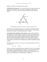
2.2 Example “Inverted Pendulum”
2.1.2 Principle of virtual work
δu
Course “Fundamentals of Structural Dynamics”
Fm
(2.13)
a sin(ϕ1)
k
Fp
• Thereby, both inertia forces and damping forces must be considered
l
(2.14)
2.1.3 Energy Formulation
a cos(ϕ1)
( f m + f c + f k )δu = F ( t )δu
Fk
a
• Kinetic energy T (Work, that an external force needs to provide to move a mass)
ϕ1
l
Course “Fundamentals of Structural Dynamics”
sin(ϕ1) ~ ϕ1
cos(ϕ1) ~ 1
• Deformation energy U (is determined from the work that an external force has to provide in order to generate a deformation)
O
• Potential energy of the external forces V (is determined with
respect to the potential energy at the position of equilibrium)
Spring force:
F k = a ⋅ sin ( ϕ 1 ) ⋅ k ≈ a ⋅ ϕ 1 ⋅ k
(2.17)
• Conservation of energy theorem (Conservative systems)
Inertia force:
··
Fm = ϕ1 ⋅ l ⋅ m
(2.18)
External force:
Fp = m ⋅ g
(2.19)
E = T + U + V = T o + U o + V o = cons tan t
(2.15)
dE
= 0
dt
(2.16)
2 Single Degree of Freedom Systems
l sin(ϕ
ϕ1)
Equilibrium
Page 2-3
F k ⋅ a ⋅ cos ( ϕ 1 ) + F m ⋅ l – F p ⋅ l ⋅ sin ( ϕ 1 ) = 0
2 Single Degree of Freedom Systems
(2.20)
Page 2-4
Course “Fundamentals of Structural Dynamics”
An-Najah 2013
2 ··
2
m ⋅ l ⋅ ϕ1 + ( a ⋅ k – m ⋅ g ⋅ l ) ⋅ ϕ1 = 0
(2.21)
Circular frequency:
K
-------1 =
M1
ω =
2
a ⋅k–m⋅g⋅l
------------------------------------- =
2
m⋅l
2
a ⋅ k- g
-----------– --2 l
m⋅l
(2.22)
An-Najah 2013
Spring force:
F k ⋅ cos ( ϕ 1 ) ≈ a ⋅ ϕ 1 ⋅ k
(2.24)
Inertia force:
··
Fm = ϕ1 ⋅ l ⋅ m
(2.25)
External force:
F p ⋅ sin ( ϕ 1 ) ≈ m ⋅ g ⋅ ϕ 1
(2.26)
δu m = δϕ 1 ⋅ l
(2.27)
Virtual displacement:
δu k = δϕ 1 ⋅ a ,
The system is stable if:
ω > 0:
Course “Fundamentals of Structural Dynamics”
2
a ⋅k>m⋅g⋅l
(2.23)
Principle of virtual work:
( F k ⋅ cos ( ϕ 1 ) ) ⋅ δu k + ( F m – ( F p ⋅ sin ( ϕ 1 ) ) ) ⋅ δu m = 0
Principle of virtual work formulation
(2.28)
··
( a ⋅ ϕ 1 ⋅ k ) ⋅ δϕ 1 ⋅ a + ( ϕ 1 ⋅ l ⋅ m – m ⋅ g ⋅ ϕ 1 ) ⋅ δϕ 1 ⋅ l = 0 (2.29)
m
Fm
Fpsin(ϕ1)
δum
Fkcos(ϕ1)
k
a
2 ··
2
m ⋅ l ⋅ ϕ1 + ( a ⋅ k – m ⋅ g ⋅ l ) ⋅ ϕ1 = 0
(2.30)
The equation of motion given by Equation (2.30) corresponds to
Equation (2.21).
δuk
l
After cancelling out δϕ 1 the following equation of motion is obtained:
ϕ1
δϕ1
sin(ϕ1) ~ ϕ1
O
2 Single Degree of Freedom Systems
cos(ϕ1) ~ 1
Page 2-5
2 Single Degree of Freedom Systems
Page 2-6
Course “Fundamentals of Structural Dynamics”
An-Najah 2013
Course “Fundamentals of Structural Dynamics”
for small angles ϕ 1 we have:
Energy Formulation
m
(1-cos(ϕ1)) l
~
0.5 l ϕ12
2
vm
2
E pot,p = – ( m ⋅ g ⋅ 0.5 ⋅ l ⋅ ϕ 1 )
l
(2.35)
and Equation (2.33) becomes:
Ekin,m
Edef,k
(2.36)
Energy conservation:
ϕ1
a
sin(ϕ1) ~ ϕ1
cos(ϕ1) ~ 1
O
1
2
2
1
Spring: E def,k = --- ⋅ k ⋅ [ a ⋅ sin ( ϕ 1 ) ] = --- ⋅ k ⋅ ( a ⋅ ϕ 1 ) (2.31)
2
2
2
2
1
1
·
E kin,m = --- ⋅ m ⋅ v m = --- ⋅ m ⋅ ( ϕ 1 ⋅ l )
2
2
(2.32)
E pot,p = – ( m ⋅ g ) ⋅ ( 1 – cos ( ϕ 1 ) ) ⋅ l
(2.33)
by means of a series development, cos ( ϕ 1 ) can be
expressed as:
2
4
2k
ϕ1 ϕ1
k
x
cos ( ϕ 1 ) = 1 – ------ + ------ – … + ( – 1 ) ⋅ ------------- + … (2.34)
2! 4!
( 2k )!
2 Single Degree of Freedom Systems
2
ϕ1
ϕ1
cos ( ϕ 1 ) = 1 – ------ and ------ = 1 – cos ( ϕ 1 )
2
2
Epot,p
a sin(ϕ1)
k
Mass:
An-Najah 2013
Page 2-7
E tot = E def,k + E kin,m + E pot,p = constant
(2.37)
2
2
2
1
·2 1
E = --- ( m ⋅ l ) ⋅ ϕ 1 + --- ( k ⋅ a – m ⋅ g ⋅ l ) ⋅ ϕ 1 = constant
2
2
(2.38)
Derivative of the energy with respect to time:
dE
= 0
dt
Derivation rule: ( g • f )' = ( g' • f ) ⋅ f'
2
2
· ··
·
( m ⋅ l ) ⋅ ϕ1 ⋅ ϕ1 + ( k ⋅ a – m ⋅ g ⋅ l ) ⋅ ϕ1 ⋅ ϕ1 = 0
(2.39)
(2.40)
·
After cancelling out the velocity ϕ 1 :
2 ··
2
m ⋅ l ⋅ ϕ1 + ( a ⋅ k – m ⋅ g ⋅ l ) ⋅ ϕ1 = 0
(2.41)
The equation of motion given by Equation (2.41) corresponds to
Equations (2.21) and (2.30).
2 Single Degree of Freedom Systems
Page 2-8
Course “Fundamentals of Structural Dynamics”
An-Najah 2013
Course “Fundamentals of Structural Dynamics”
An-Najah 2013
2.3 Modelling
Comparison of the energy maxima
2
1
·
KE = --- ⋅ m ⋅ ( ϕ 1,max ⋅ l )
2
(2.42)
2.3.1 Structures with concentrated mass
2
2 1
1
PE = --- ⋅ k ⋅ ( a ⋅ ϕ 1 ) – --- ⋅ g ⋅ m ⋅ l ⋅ ϕ 1
2
2
(2.43)
Tank:
Mass=1000t
Water tank
F(t)
F(t)
By equating KE and PE we obtain:
RC Walls in the
longitudinal direction
§ 2 ⋅ k – m ⋅ g ⋅ l·
·
ϕ 1,max = ¨ a------------------------------------¸ ⋅ ϕ 1
2
©
¹
m⋅l
(2.44)
·
ϕ 1,max = ω ⋅ ϕ 1
(2.45)
• ω is independent of the initial angle ϕ 1
Ground
Tra
dir nsver
ect se
ion
al
din
itu n
ng ctio
o
L ire
d
Bridge in transverse direction
• the greater the deflection, the greater the maximum velocity.
k = …
3EI w
k = 2 ----------3
H
F(t)
Frame with rigid beam
3EI w
k = ----------3
H
F(t)
12EI s
k = 2 ------------3
H
mu·· + ku = F ( t )
2 Single Degree of Freedom Systems
Page 2-9
2 Single Degree of Freedom Systems
(2.46)
Page 2-10
Course “Fundamentals of Structural Dynamics”
An-Najah 2013
2.3.2 Structures with distributed mass
Course “Fundamentals of Structural Dynamics”
δA i =
An-Najah 2013
L
³0 ( EIu'' ⋅ δ [ u'' ] ) dx
(2.53)
• Transformations:
u'' = ψ''U
··
u·· = ψU
and
(2.54)
• The virtual displacement is affine to the selected deformation:
δu = ψδU
δ [ u'' ] = ψ''δU
and
(2.55)
• Using Equations (2.54) and (2.55), the work δA a produced by the
external forces is:
u ( x, t ) = ψ ( x )U ( t )
Deformation:
External forces:
t ( x, t ) = – mu··( x, t )
f ( x, t )
(2.47)
0
(2.48)
• Principle of virtual work
δA i = δA a
L
³0
δA a =
(2.49)
L
( t ⋅ δu ) dx + ³ ( f ⋅ δu ) dx
(2.50)
(2.56)
0
·· L mψ 2 dx + L fψ dx
= δU – U
³
³
0
0
• Using Equations (2.54) and (2.55) the work δA i produced by the
internal forces is:
δA i =
L
³0
L
( EIψ''U ⋅ ψ''δU ) dx = δU U ³ ( EI ( ψ'' ) 2 ) dx
(2.57)
0
L
0
L
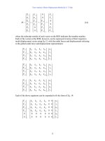
• Equation (2.49) is valid for all virtual displacements, therefore:
0
0
L
·· L mψ 2 dx + L fψ dx
U ³ ( EI ( ψ'' ) 2 ) dx = – U
³
³
(2.58)
* ··
*
*
m U
+k U = F
(2.59)
= – ³ ( mu·· ⋅ δu ) dx + ³ ( f ⋅ δu ) dx
δA i =
L
·· ⋅ ψδU ) dx + L ( f ⋅ ψδU ) dx
δA a = – ³ ( mψU
³
0
L
³0 ( M ⋅ δϕ ) dx where:
M = EIu''
and
2 Single Degree of Freedom Systems
δϕ = δ [ u'' ]
(2.51)
0
0
(2.52)
Page 2-11
2 Single Degree of Freedom Systems
Page 2-12
Course “Fundamentals of Structural Dynamics”
An-Najah 2013
Course “Fundamentals of Structural Dynamics”
An-Najah 2013
• Example No. 1: Cantilever with distributed mass
• Circular frequency
L
2
ωn
*
³0 ( EI ( ψ'' ) 2 ) dx
k
= ------*- = -----------------------------------L
2
m
³ mψ dx
(2.60)
0
-> Rayleigh-Quotient
• Choosing the deformation figure
- The accuracy of the modelling depends on the assumed
deformation figure;
- The best results are obtained when the deformation figure
fulfills all boundary conditions;
- The boundary conditions are automatically satisfied if the
deformation figure corresponds to the deformed shape due
to an external force;
- A possible external force is the weight of the structure acting in the considered direction.
• Properties of the Rayleigh-Quotient
- The estimated natural frequency is always larger than the
exact one (Minimization of the quotient!);
- Useful results can be obtained even if the assumed deformation figure is not very realistic.
2 Single Degree of Freedom Systems
Page 2-13
πx
π 2
ψ'' = § -------· cos § -------·
© 2L¹
© 2L¹
πx
ψ = 1 – cos § -------· ,
© 2L¹
*
m =
L
§
§ πx· · dx + ψ 2 ( x = L )M
³0 m © 1 – cos © -----2L¹ ¹
2
πx-·
πx
πx
§ 3πx – 8 sin § -----L + 2 cos § -------· sin § -------· L·
© 2L¹
© 2L¹ © 2L¹ ¸
1--- ¨
= m ¨ ----------------------------------------------------------------------------------------------------¸
2 ¨
π
¸
©
¹
(2.61)
(2.62)
L
+M
0
( 3π – 8 )
= -------------------- mL + M = 0.23mL + M
2π
2 Single Degree of Freedom Systems
Page 2-14
Course “Fundamentals of Structural Dynamics”
An-Najah 2013
Course “Fundamentals of Structural Dynamics”
An-Najah 2013
• Example No. 2: Cantilever with distributed mass
*
πx 2
π 4 L
k = EI § -------· ³ § cos § -------· · dx
© 2L¹ ¹
© 2L¹ 0 ©
πx· § πx· ·
§ πx + 2 cos § ------ sin ------- L
4
©
¹ © 2L¹ ¸
¨
2L
1
π
§
·
= EI ------- ⋅ --- ¨ ---------------------------------------------------------------¸
© 2L¹ 2 ¨
π
¸
©
¹
(2.63)
L
0
4
EI 3EI
π EI
= ------ ⋅ -----3- = 3.04 ⋅ -----3- ≈ -------3
32 L
L
L
ω =
πx
ψ = 1 – cos § -------· ,
© 2L¹
3EI
----------------------------------------3
( 0.23mL + M )L
(2.64)
• Check of the boundary conditions of the deformation figure
πx
ψ ( 0 ) = 0 ? -> ψ ( x ) = 1 – cos §© -------·¹ :
2L
ψ ( 0 ) = 0 OK!
π
πx
ψ' ( 0 ) = 0 ? -> ψ' ( x ) = ------- sin §© -------·¹ :
2L
2L
ψ' ( 0 ) = 0 OK!
π 2
πx
ψ'' ( L ) = 0 ? -> ψ'' ( x ) = §© -------·¹ cos §© -------·¹ :
2L
2L
ψ'' ( L ) = 0 OK!
• Calculation of the mass m
*
m =
L
§
πx
π 2
ψ'' = § -------· cos § -------·
© 2L¹
© 2L¹
*
2
§ πx· · dx + ψ 2 § x = L
---· M 1 + ψ 2 ( x = L )M 2
©
2¹
³0 m © 1 – cos © -----2L¹ ¹
(2.67)
( 3π – 8 )
3–2 2
*
m = -------------------- mL + § -------------------· ⋅ M 1 + M 2
© 2 ¹
2π
(2.68)
*
Page 2-15
(2.66)
( 3π – 8 )
π 2
*
2
m = -------------------- mL + § 1 – cos § ---· · ⋅ M 1 + 1 ⋅ M 2
©
©
4¹ ¹
2π
m = 0.23mL + 0.086M 1 + M 2
2 Single Degree of Freedom Systems
(2.65)
2 Single Degree of Freedom Systems
(2.69)
Page 2-16
Course “Fundamentals of Structural Dynamics”
• Calculation of the stiffness k
*
*
πx 2
π 4 L
k = EI § -------· ³ § cos § -------· · dx
© 2L¹ ¹
© 2L¹ 0 ©
6
3.04EI
------------------------------------------------------------------------3
( 0.23mL + 0.086M 1 + M 2 )L
4
(2.70)
(2.71)
(2.72)
3.04EI
EI
------------------------------ = 1.673 ----------3
3
( 1.086M )L
ML
3.007EI - = 1.652 ----------EI
----------------------------3
3
( 1.102M )L
ML
(2.73)
(2.74)
As a numerical example, the first natural frequency of a
L = 10m tall steel shape HEB360 (bending about the strong axis) featuring two masses M 1 = M 2 = 10t is calculated.
2 Single Degree of Freedom Systems
2
2
(2.75)
(2.76)
4
EI = 1.673 -----------------------8.638 ×10 - = 4.9170
ω = 1.673 ----------3
3
10 ⋅ 10
ML
(2.77)
1
4.9170
f = ------ ⋅ ω = ---------------- = 0.783Hz
2π
2π
(2.78)
From Equation (2.74):
1.652 EI
1.652 8.638 ×10⁴
f = ------------- ----------= ------------- ------------------------ = 0.773Hz
3
2π ML 3
2π
10 ⋅ 10
The exact first natural circular frequency of a two-mass oscillator
with constant stiffness and mass is:
ω =
EI = 8.638 ×10 kNm
An-Najah 2013
By means of Equation (2.73) we obtain:
Special case: m = 0 and M 1 = M 2 = M
ω =
13
EI = 200000 ⋅ 431.9 ×10 = 8.638 ×10 Nmm
• Calculation of the circular frequency ω
ω =
Course “Fundamentals of Structural Dynamics”
4
EI 3EIπ EI
k = ------ ⋅ -----3- = 3.04 ⋅ -----3- ≈ -------3
32 L
L
L
*
An-Najah 2013
Page 2-17
(2.79)
The first natural frequency of such a dynamic system can be calculated using a finite element program (e.g. SAP 2000), and it is
equal to:
T = 1.2946s , f = 0.772Hz
(2.80)
Equations (2.78), (2.79) and (2.80) are in very good accordance.
The representation of the first mode shape and corresponding
natural frequency obtained by means of a finite element program
is shown in the next figure.
2 Single Degree of Freedom Systems
Page 2-18
Course “Fundamentals of Structural Dynamics”
An-Najah 2013
Course “Fundamentals of Structural Dynamics”
An-Najah 2013
2.3.3 Damping
• Types of damping
M = 10t
Damping
Internal
Material
Hysteretic
(Viscous,
Friction,
Yielding)
M = 10t
External
Contact areas
within the structure
Relative
movements
between parts of
the structure
(Bearings, Joints,
etc.)
External contact
(Non-structural
elements, Energy
radiation in the
ground, etc.)
• Typical values of damping in structures
Damping ζ
Material
Reinforced concrete (uncraked)
Reinforced concrete (craked
Reinforced concrete (PT)
Reinforced concrete (partially PT)
Composite components
Steel
HEB 360
0.007 - 0.010
0.010 - 0.040
0.004 - 0.007
0.008 - 0.012
0.002 - 0.003
0.001 - 0.002
Table C.1 from [Bac+97]
SAP2000 v8 - File:HEB_360 - Mode 1 Period 1.2946 seconds - KN-m Units
2 Single Degree of Freedom Systems
Page 2-19
2 Single Degree of Freedom Systems
Page 2-20
Course “Fundamentals of Structural Dynamics”
An-Najah 2013
• Bearings
An-Najah 2013
• Dissipators
Source: A. Marioni: “Innovative Anti-seismic Devices for Bridges”.
[SIA03]
2 Single Degree of Freedom Systems
Course “Fundamentals of Structural Dynamics”
Page 2-21
Source: A. Marioni: “Innovative Anti-seismic Devices for Bridges”.
[SIA03]
2 Single Degree of Freedom Systems
Page 2-22
Course “Fundamentals of Structural Dynamics”
An-Najah 2013
3 Free Vibrations
Course “Fundamentals of Structural Dynamics”
An-Najah 2013
• Relationships
“A structure undergoes free vibrations when it is brought out of
its static equilibrium, and can then oscillate without any external
dynamic excitation”
ωn =
ωn
f n = ------ [1/s], [Hz]: Number of revolutions per time
2π
(3.8)
3.1 Undamped free vibrations
2π
T n = ------ [s]:
ωn
(3.9)
mu··( t ) + ku ( t ) = 0
(3.1)
k ⁄ m [rad/s]: Angular velocity
Time required per revolution
(3.7)
• Transformation of the equation of motion
3.1.1 Formulation 1: Amplitude and phase angle
2
u··( t ) + ω n u ( t ) = 0
• Ansatz:
(3.10)
• Determination of the unknowns A and φ :
u ( t ) = A cos ( ω n t – φ )
(3.2)
2
u··( t ) = – A ω n cos ( ω n t – φ )
(3.3)
The static equilibrium is disturbed by the initial displacement
u ( 0 ) = u 0 and the initial velocity u· ( 0 ) = v 0 :
(3.4)
A =
By substituting Equations (3.2) and (3.3) in (3.1):
2
A ( – ω n m + k ) cos ( ω n t – φ ) = 0
2
– ωn m + k = 0
(3.5)
ωn =
(3.6)
k ⁄ m “Natural circular frequency”
3 Free Vibrations
Page 3-1
v0 2
v0
2
u 0 + § ------· , tan φ = ----------© ω n¹
u0 ωn
(3.11)
• Visualization of the solution by means of the Excel file given on
the web page of the course (SD_FV_viscous.xlsx)
3 Free Vibrations
Page 3-2
Course “Fundamentals of Structural Dynamics”
An-Najah 2013
3.1.2 Formulation 2: Trigonometric functions
mu··( t ) + ku ( t ) = 0
Course “Fundamentals of Structural Dynamics”
An-Najah 2013
3.1.3 Formulation 3: Exponential Functions
(3.12)
• Ansatz:
mu··( t ) + ku ( t ) = 0
(3.19)
• Ansatz:
u ( t ) = A 1 cos ( ω n t ) + A 2 sin ( ω n t )
(3.13)
u(t) = e
2
2
u··( t ) = – A 1 ω n cos ( ω n t ) – A 2 ω n sin ( ω n t )
(3.14)
2 λt
u··( t ) = λ e
By substituting Equations (3.13) and (3.14) in (3.12):
2
2
– ωn m + k = 0
(3.16)
ωn =
(3.17)
k ⁄ m “Natural circular frequency”
• Determination of the unknowns A 1 and A 2 :
2
mλ + k = 0
(3.22)
2
k
λ = – ---m
(3.23)
k- = ± iω
λ = ± i --n
m
(3.24)
u ( t ) = C1 e
iω n t
+ C2 e
–i ωn t
(3.25)
and by means of Euler’s formulas
(3.18)
iα
Page 3-3
–i α
iα
–i α
e +e
e –e
cos α = ----------------------- , sin α = ----------------------2
2i
e
3 Free Vibrations
(3.21)
The complete solution of the ODE is:
The static equilibrium is disturbed by the initial displacement
u ( 0 ) = u 0 and the initial velocity u· ( 0 ) = v 0 :
v0
A 1 = u 0 , A 2 = -----ωn
(3.20)
By substituting Equations (3.20) and (3.21) in (3.19):
A 1 ( – ω n m + k ) cos ( ω n t ) + A 2 ( – ω n m + k ) sin ( ω n t ) = 0 (3.15)
2
λt
iα
= cos ( α ) + i sin ( α ) , e
3 Free Vibrations
–i α
= cos ( α ) – i sin ( α )
(3.26)
(3.27)
Page 3-4
Course “Fundamentals of Structural Dynamics”
An-Najah 2013
Course “Fundamentals of Structural Dynamics”
An-Najah 2013
3.2 Damped free vibrations
Equation (3.25) can be transformed as follows:
u ( t ) = ( C 1 + C 2 ) cos ( ω n t ) + i ( C 1 – C 2 ) sin ( ω n t )
(3.28)
mu··( t ) + cu· ( t ) + ku ( t ) = 0
u ( t ) = A 1 cos ( ω n t ) + A 2 sin ( ω n t )
(3.29)
- In reality vibrations subside
(3.30)
- Damping exists
Equation (3.29) corresponds to (3.13)!
- It is virtually impossible to model damping exactly
- From the mathematical point of view viscous damping is
easy to treat
s
Damping constant: c N ⋅ ---m
(3.31)
3.2.1 Formulation 3: Exponential Functions
mu··( t ) + cu· ( t ) + ku ( t ) = 0
(3.32)
• Ansatz:
u(t) = e
λt
λt
2 λt
, u· ( t ) = λe , u··( t ) = λ e
(3.33)
By substituting Equations (3.33) in (3.32):
2
( λ m + λc + k )e
λt
= 0
2
3 Free Vibrations
Page 3-5
(3.34)
λ m + λc + k = 0
(3.35)
2
c
1
λ = – -------- ± -------- c – 4km
2m 2m
(3.36)
3 Free Vibrations
Page 3-6
Course “Fundamentals of Structural Dynamics”
An-Najah 2013
An-Najah 2013
• Types of vibrations
• Critical damping when: c 2 – 4km = 0
c cr = 2 km = 2ω n m
Course “Fundamentals of Structural Dynamics”
1
(3.37)
Underdamped vibration
Critically damped vibration
• Damping ratio
Overdamped vibration
(3.38)
• Transformation of the equation of motion
mu··( t ) + cu· ( t ) + ku ( t ) = 0
(3.39)
c
k
u··( t ) + ---- u· ( t ) + ---- u ( t ) = 0
m
m
(3.40)
2
u··( t ) + 2ζω n u· ( t ) + ω n u ( t ) = 0
(3.41)
u(t)/u0 [-]
c
c
c
ζ = ------ = --------------- = -------------2ω
c cr
2 km
nm
0.5
0
-0.5
-1
• Types of vibrations:
0.5
1
1.5
2
2.5
3
3.5
4
t/Tn [-]
c
ζ = ------ < 1 :
c cr
Underdamped free vibrations
c
ζ = ------ = 1 :
c cr
Critically damped free vibrations
c
ζ = ------ > 1 :
c cr
Overdamped free vibrations
3 Free Vibrations
0
Page 3-7
3 Free Vibrations
Page 3-8
Course “Fundamentals of Structural Dynamics”
An-Najah 2013
Underdamped free vibrations ζ < 1
Course “Fundamentals of Structural Dynamics”
An-Najah 2013
The determination of the unknowns A 1 and A 2 is carried out as
usual by means of the initial conditions for displacement
( u ( 0 ) = u 0 ) and velocity ( u· ( 0 ) = v 0 ) obtaining:
By substituting:
2
c
c
k
c
ζ = ------ = --------------- = --------------- and ω n = ---2ω n m
m
c cr
2 km
(3.42)
v 0 + ζω n u 0
A 1 = u 0 , A 2 = --------------------------ωd
(3.51)
in:
c
1
c
c 2 k
2
λ = – -------- ± -------- c – 4km = – -------- ± § --------· – ---© 2m¹
m
2m 2m
2m
3.2.2 Formulation 1: Amplitude and phase angle
(3.43)
Equation (3.50) can be rewritten as “the amplitude and phase
angle”:
it is obtained:
2 2
2
2
λ = – ζω n ± ω n ζ – ω n = – ζω n ± ω n ζ – 1
λ = – ζω n ± iω n 1 – ζ
2
u ( t ) = Ae
(3.44)
A =
ω d = ω n 1 – ζ “damped circular frequency”
(3.46)
λ = – ζω n ± iω d
(3.47)
The complete solution of the ODE is:
u ( t ) = C1 e
u(t) = e
u(t) = e
3 Free Vibrations
( – ζω n + iω d )t
– ζω n t
– ζω n t
( C1 e
iω d t
+ C2 e
+ C2 e
( – ζω n – iω d )t
–i ωd t
)
( A 1 cos ( ω d t ) + A 2 sin ( ω d t ) )
cos ( ω d t – φ )
(3.52)
with
(3.45)
2
– ζω n t
v 0 + ζω n u 0
v 0 + ζω n u 0 2
2
u 0 + § ---------------------------· , tan φ = --------------------------©
¹
ωd
ωd u0
(3.53)
The motion is a sinusoidal vibration with
circular frequency ω d and decreasing amplitude Ae
– ζω n t
(3.48)
(3.49)
(3.50)
Page 3-9
3 Free Vibrations
Page 3-10
Course “Fundamentals of Structural Dynamics”
An-Najah 2013
Course “Fundamentals of Structural Dynamics”
3.3 The logarithmic decrement
• Notes
- The period of the damped vibration is longer, i.e. the vibration is slower
20
Td
u0
15
1
Free vibration
u1
10
0.8
0.7
0.6
ωd = ωn 1 – ζ
0.5
2
Tn
T d = -----------------2
1–ζ
0.4
0.3
03
Displacement
0.9
Tn/Td
An-Najah 2013
5
0
-5
-10
-15
0.2
-20
0.1
0
1
2
3
4
5
6
7
8
9
10
Time (s)
0
0
0.1 0.2 0.3 0.4 0.5 0.6 0.7 0.8 0.9
1
Damping ratio ζ
• Amplitude of two consecutive cycles
- The envelope of the vibration is represented by the following equation:
u ( t ) = Ae
– ζω n t
with A =
v 0 + ζω n u 0 2
2
u 0 + § ---------------------------·
©
¹
ωd
(3.54)
- Visualization of the solution by means of the Excel file given on the web page of the course (SD_FV_viscous.xlsx)
3 Free Vibrations
Page 3-11
– ζω t
n
u0
cos ( ω d t – φ )
Ae
----- = -------------------------------------------------------------------------------–
ζω
(
t
+
T
)
d
u1
Ae n
cos ( ω d ( t + T d ) – φ )
(3.55)
with
e
– ζω n ( t + T d )
= e
– ζω n t – ζω n T d
e
cos ( ω d ( t + T d ) – φ ) = cos ( ω d t + ω d T d – φ ) = cos ( ω d t – φ )
3 Free Vibrations
(3.56)
(3.57)
Page 3-12
Course “Fundamentals of Structural Dynamics”
An-Najah 2013
we obtain:
An-Najah 2013
• Evaluation over several cycles
u0
ζω T
1
----- = ----------------- = e n d
–
ζω
T
n
d
u1
e
(3.58)
• Logarithmic decrement δ
u0
2πζ
δ = ln § -----· = ζω n T d = ------------------ ≅ 2πζ (if ζ small)
© u 1¹
2
1–ζ
(3.59)
The damping ratio becomes:
δ
δ
ζ = ------------------------- ≅ ------ (if ζ small)
2
2 2π
4π + δ
(3.60)
u u
uN – 1
u
ζω T N
Nζω n T d
-----0- = ----0- ⋅ ----1- ⋅ … ⋅ ------------ = (e n d) = e
uN
u1 u2
uN
(3.61)
u0
1
δ = ---- ln § ------·
N © u N¹
(3.62)
• Halving of the amplitude
u
1
---- ln § -----0-·
N © u N¹
ζ = ---------------------- =
2π
1
---- ln ( 2 )
N
1 - --------1------------------ = -----≅
2π
9N 10N
(3.63)
Useful formula for quick evaluation
10
Exact equation
9
Logarithmic Decrement δ
Course “Fundamentals of Structural Dynamics”
• Watch out: damping ratio vs. damping constant
Approximation
8
Empty
7
Full
6
5
4
3
2
1
0
0
0.1
0.2
0.3
0.4
0.5
0.6
0.7
0.8
0.9
1
Damping ratio ζ
3 Free Vibrations
Page 3-13
m 1, k 1, c 1
m2>m1, k1, c1
c1
ζ 1 = -------------------2 k1 m1
c1
ζ 2 = -------------------- < ζ 1
2 k1 m2
3 Free Vibrations
Page 3-14