Fundamentals of Structural Analysis P1 docx

Fundamentals
of
Structural Analysis
S. T. Mau
ii
Copyright registration number TXu1-086-529, February 17, 2003.
United States Copyright Office, The Library of Congress
This book is intended for the use of individual students and teachers.
No part of this book may be reproduced, in any form or by any means, for commercial
purposes, without permission in writing from the author.
iii
Contents
Preface v
Truss Analysis: Matrix Displacement Method 1
1. What is a Truss? 1
2. A Truss Member 3
3. Member Stiffness Equation in Global Coordinates 4
Problem 1. 11
4. Unconstrained Global Stiffness Equation 11
5. Constrained Global Stiffness Equation and Its Solution 17
Problem 2. 19
6. Procedures of Truss Analysis 20
Problem 3. 27
7. Kinematic Stability 27
Problem 4. 29
8. Summary 30
Truss Analysis: Force Method, Part I 31
1. Introduction 31
2. Statically Determinate Plane Truss types 31
3. Method of Joint and Method of Section 33
Problem 1. 43

Problem 2. 55
4. Matrix Method of Joint 56
Problem 3. 61
Problem 4. 66
Truss Analysis: Force Method, Part II 67
5. Truss Deflection 67
Problem 5. 81
6. Indeterminate Truss Problems – Method of Consistent Deformations 82
7. Laws of Reciprocity 89
8. Concluding Remarks 90
Problem 6. 91
Beam and Frame Analysis: Force Method, Part I 93
1. What are Beams and Frames? 93
2. Statical Determinacy and Kinematic Stability 94
Problem 1. 101
3. Shear and Moment Diagrams 102
4. Statically Determinate Beams and Frames 109
Problem 2. 118
Beam and Frame Analysis: Force Method, Part II 121
5. Deflection of Beam and Frames 121
Problem 3. 132
iv
Problem 4. 143
Problem 5. 152
Beam and Frame Analysis: Force Method, Part III 153
6. Statically Indeterminate Beams and Frames 153
Table: Beam Deflection Formulas 168
Problem 6. 173
Beam and Frame Analysis: Displacement Method, Part I 175
1. Introduction 175

2. Moment Distribution Method 175
Problem 1. 207
Table: Fixed End Moments 208
Beam and Frame Analysis: Displacement Method, Part II 209
3. Slope-Deflection Method 209
Problem 2. 232
4. Matrix Stiffness Analysis of Frames 233
Problem 3. 248
Influence Lines 249
1. What is Influence Line? 249
2. Beam Influence Lines 250
Problem 1. 262
3. Truss Influence Lines 263
Problem 2. 271
Other Topics 273
1. Introduction 273
2. Non-Prismatic Beam and Frames Members 273
Problem 1. 277
3. Support Movement, Temperature, and Construction Error Effects 278
Problem 2. 283
4. Secondary Stresses in Trusses 283
5. Composite Structures 285
6. Materials Non-linearity 287
7. Geometric Non-linearity 288
8. Structural Stability 290
9. Dynamic Effects 294
Matrix Algebra Review 299
1. What is a Matrix? 299
2. Matrix Operating Rules 300
3. Matrix Inversion and Solving Simultaneous Algebraic Equations 302

Problem 307
Solution to Problems 309
Index 323
v
Preface
There are two new developments in the last twenty years in the civil engineering
curricula that have a direct bearing on the design of the content of a course in structural
analysis: the reduction of credit hours to three required hours in structural analysis in
most civil engineering curricula and the increasing gap between what is taught in
textbooks and classrooms and what is being practiced in engineering firms. The former is
brought about by the recognition of civil engineering educators that structural analysis as
a required course for all civil engineering majors need not cover in great detail all the
analytical methods. The latter is certainly the result of the ubiquitous applications of
personal digital computer.
This structural analysis text is designed to bridge the gap between engineering practice
and education. Acknowledging the fact that virtually all computer structural analysis
programs are based on the matrix displacement method of analysis, the text begins with
the matrix displacement method. A matrix operations tutorial is included as a review and
a self-learning tool. To minimize the conceptual difficulty a student may have in the
displacement method, it is introduced with plane truss analysis, where the concept of
nodal displacements presents itself. Introducing the matrix displacement method early
also makes it easier for students to work on term project assignments that involve the
utilization of computer programs.
The force method of analysis for plane trusses is then introduced to provide the coverage
of force equilibrium, deflection, statical indeterminacy, etc., that are important in the
understanding of the behavior of a structure and the development of a feel for it.
The force method of analysis is then extended to beam and rigid frame analysis, almost in
parallel to the topics covered in truss analysis. The beam and rigid frame analysis is
presented in an integrated way so that all the important concepts are covered concisely
without undue duplicity.

The displacement method then re-appears when the moment distribution and slope-
deflection methods are presented as a prelude to the matrix displacement method for
beam and rigid frame analysis. The matrix displacement method is presented as a
generalization of the slope-deflection method.
The above description outlines the introduction of the two fundamental methods of
structural analysis, the displacement method and the force method, and their applications
to the two groups of structures, trusses and beams-and-rigid frames. Other related topics
such as influence lines, non-prismatic members, composite structures, secondary stress
analysis, limits of linear and static structural analysis are presented at the end.
S. T. Mau
2002
vi
1
Truss Analysis: Matrix Displacement Method
1. What Is a Truss?
In a plane, a truss is composed of relatively slender members often forming triangular
configurations. An example of a plane truss used in the roof structure of a house is
shown below.
A roof truss called Fink truss.
The circular symbol in the figure represents a type of connection called hinge, which
allows members to rotate in the plane relatively to each other at the connection but not to
move in translation against each other. A hinge connection transmits forces from one
member to the other but not force couple, or moment, from one member to the other.
In real construction, a plane truss is most likely a part of a structure in the three-
dimensional space we know. An example of a roof structure is shown herein. The
bracing members are needed to connect two plane trusses together. The purlins and
rafters are for the distribution of roof load to the plane trusses.
A roof structure with two Fink trusses.
Bracing
Rafter

Purlin
Truss Analysis: Matrix Displacement Method by S. T. Mau
2
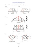
Some other truss types seen in roof or bridge structures are shown below.
Different types of plane trusses.
Saw-tooth Truss
Three-hinged Arch
Parker Truss: Pratt with curved chord
K Truss
Deck Pratt Truss
Warren Truss
Pratt Truss
Howe Truss
Truss Analysis: Matrix Displacement Method by S. T. Mau
3
2. A Truss Member
Each member of a truss is a straight element, taking loads only at the two ends. As a
result, the two forces at the two ends must act along the axis of the member and of the
same magnitude in order to achieve equilibrium of the member as shown in the figures
below.
Truss member in equilibrium. Truss member not in equilibrium.
Furthermore, when a truss member is in equilibrium, the two end forces are either
pointing away from each other or against each other, creating tension or compression,
respectively in the member.

Truss member in tension Truss member in compression
Whether a member is in tension or compression, the internal force acting on any chosen
section of the member is the same throughout the member. Thus, the state of force in the
member can be represented by a single member force entity, represented by the notation
F, which is the axial member force of a truss member. There are no other member forces

in a trusss member.
F
F
F
F
Truss Analysis: Matrix Displacement Method by S. T. Mau
4
The internal force is the same at any section of a truss member.
A tensile member force is signified by a positive value in F and a compressive member
force is signified by a negative value in F. This is the sign convention for the member
force of an axial member.
Whenever there is force in a member, the member will deform. Each segment of the
member will elongate, or shorten and the cumulative effect of the deformation is a
member elongation, or shortening,
∆
.


Member elongation.
Assuming the material the member is made of is linearly elastic with Young’s modulus
E, and the member is prismatic with a constant cross-sectional area, A and length L, then
the relationship between the member elongation and member force can be shown to be:
F = k
∆
with
L
EA
k =
(1)
where the proportional factor k is called the member rigidity. Eq. 1 is the member

stiffness equation expressed in local coordinate, namely the axial coordinate. This
relationship will eventually be expressed in a coordinate system that is common to all
members in a truss, i.e., a global coordinate system. For this to be done, we must
examine the relative position of a member in the truss.
3. Member Stiffness Equation in Global Coordinates
The simplest truss is a three-member truss as shown. Once we have defined a global
coordinate system, the x-y system, then the displaced configuration of the whole structure
is completely determined by the nodal displacement pairs (u
1
, v
1
), (u
2
, v
2
), and (u
3
, v
3
).
y
∆
F
Truss Analysis: Matrix Displacement Method by S. T. Mau
5
A three-member truss Nodal displacements in global coordinates
Furthermore, the elongation of a member can be calculated from the nodal displacements.
Displaced member Overlapped configurations
∆
= (u

2
-u
1
) Cos
θ
+ (v
2
-v
1
) Sin
θ
(2)
or,
∆
= -(Cos
θ
) u
1
–( Sin
θ
) v
1
+ (Cos
θ
) u
2
+(Sin
θ
)

v
2
(2)
In the above equation, it is understood that the angle
θ
refers to the orientation of member
1-2. For brevity we did not include the subscript that designates the member. We can
express the same equation in a matrix form, letting C and S represent Cos
θ
and Sin
θ
respectively.
∆
=
⎣⎦
SCSC −−
⎪
⎪
⎭
⎪
⎪
⎬
⎫
⎪
⎪
⎩
⎪
⎪
⎨
⎧

2
2
1
1
v
u
v
u
(3)
Again, the subscript “1-2” is not included for
∆
, C and S for brevity. One of the
advantages of using the matrix form is that the functional relationship between the
member elongation and the nodal displacement is clearer than that in the expression in
Eq. 2. Thus, the above equation can be cast as a transformation between the local quantity
of deformation
∆
L
=
∆
and the global nodal displacements
∆
G
:
θ
θ
∆
2’
2
u

2
-u
1
v
2
-v
1
x
2’
2
1 1’
1’
1
2
2’
v
3
u
3
3
2
1
x
Truss Analysis: Matrix Displacement Method by S. T. Mau
6
∆
L
=
Γ

∆
G
(4)
where
Γ
=
⎣⎦
SCSC −−
(5)
and
∆
G
=
⎪
⎪
⎭
⎪
⎪
⎬
⎫
⎪
⎪
⎩
⎪
⎪
⎨
⎧
2
2
1

1
v
u
v
u
(6)
Here and elsewhere a boldfaced symbol represents a vector or a matrix. Eq. 4 is the
deformation transformation equation. We now seek the transformation between the
member force in local coordinate, F
L
=F and the nodal forces in the x-y coordinates, F
G
.
Member force F and nodal forces in global coordinates.
From the above figure and the equivalence of the two force systems, we obtain
F
G
=
⎪
⎪
⎭
⎪
⎪
⎬
⎫
⎪
⎪
⎩
⎪
⎪

⎨
⎧
2
2
1
1
y
x
y
x
F
F
F
F
=
⎪
⎪
⎭
⎪
⎪
⎬
⎫
⎪
⎪
⎩
⎪
⎪
⎨
⎧
−

−
S
C
S
C
F (7)
where C and S represent the cosine and sine of the member orientation angle
θ
. Noting
that the transformation vector is the transpose of
Γ
, we can re-write Eq. 7 as
F
G
=
Γ

T
F
L
(8)
Eq. 8 is the force transformation equation.
x
y
F
x1
F
x2
F
y2

F
y1
F
θ
F
=
Truss Analysis: Matrix Displacement Method by S. T. Mau
7
By simple substitution, using Eq. 1 and Eq. 4, the above force transformation equation
leads to
F
G
=
Γ

T
F
L
=
Γ

Τ
k
∆
L
=
Γ

Τ
k

Γ

∆
G
or,
F
G
= k
G
∆
G
(9)
where
k
G
=
Γ

Τ
k
Γ
(10)
The above equation is the stiffness transformation equation, which transforms the
member stiffness in local coordinate, k, into the member stiffness in global coordinate,
k
G
. In the expanded form, i.e. when the triple multiplication in the above equation is
carried out, the member stiffness is a 4x4 matrix:
k
G

=
⎥
⎥
⎥
⎥
⎥
⎦
⎤
⎢
⎢
⎢
⎢
⎢
⎣
⎡
−−
−−
−−
−−
22
22
22
22
SCSSCS
CSCCSC
SCSSCS
CSCCSC
L
EA
(11)

The meaning of each of the component of the matrix, (k
G
)
ij
, can be explored by
considering the nodal forces corresponding to the following four sets of “unit” nodal
displacements:
Truss Analysis: Matrix Displacement Method by S. T. Mau
8

∆
G
=
⎪
⎪
⎭
⎪
⎪
⎬
⎫
⎪
⎪
⎩
⎪
⎪
⎨
⎧
2
2
1

1
v
u
v
u
=
⎪
⎪
⎭
⎪
⎪
⎬
⎫
⎪
⎪
⎩
⎪
⎪
⎨
⎧
0
0
0
1

∆
G
=
⎪
⎪

⎭
⎪
⎪
⎬
⎫
⎪
⎪
⎩
⎪
⎪
⎨
⎧
2
2
1
1
v
u
v
u
=
⎪
⎪
⎭
⎪
⎪
⎬
⎫
⎪
⎪

⎩
⎪
⎪
⎨
⎧
0
0
1
0

∆
G
=
⎪
⎪
⎭
⎪
⎪
⎬
⎫
⎪
⎪
⎩
⎪
⎪
⎨
⎧
2
2
1

1
v
u
v
u
=
⎪
⎪
⎭
⎪
⎪
⎬
⎫
⎪
⎪
⎩
⎪
⎪
⎨
⎧
0
1
0
0

∆
G
=
⎪
⎪

⎭
⎪
⎪
⎬
⎫
⎪
⎪
⎩
⎪
⎪
⎨
⎧
2
2
1
1
v
u
v
u
=
⎪
⎪
⎭
⎪
⎪
⎬
⎫
⎪
⎪

⎩
⎪
⎪
⎨
⎧
1
0
0
0
Four sets of unit nodal displacements
When each of the above “unit” displacement vector is multiplied by the stiffness matrix
according to Eq. 9, it becomes clear that the resulting nodal forces are identical to the
components of one of the columns of the stiffness matrix. For example, the first column
of the stiffness matrix contains the nodal forces needed to produce a unit displacement in
u
1
, with all other nodal displacements being zero. Furthermore, we can see (k
G
)
ij
is the ith
nodal force due to a unit displacement at the jth nodal displacement.
By examining Eq. 11, we observe the following features of the stiffness matrix:
1
2
1
2
1
2
1

2
Truss Analysis: Matrix Displacement Method by S. T. Mau
9
(a) The member stiffness matrix is symmetric, (k
G
)
ij
= (k
G
)
ji
.
(b) The algebraic sum of the components in each column or each row is zero.
(c) The member stiffness matrix is singular.
Feature (a) can be traced to the way the matrix is formed, via Eq.10, which invariably
leads to a symmetric matrix. Feature (b) comes from the fact that nodal forces due to a
set of unit nodal displacements must be in equilibrium. Feature (c) is due to the
proportionality of the pair of columns 1 and 3, or 2 and 4.
The fact that member stiffness matrix is singular and therefore cannot be inverted
indicates that we cannot solve for the nodal displacements corresponding to any given set
of nodal forces. This is because the given set of nodal forces may not be in equilibrium
and therefore it is not meaningful to ask for the corresponding nodal displacements. Even
if they are in equilibrium, the solution of nodal displacements requires a special
procedure described under “eigenvalue problems” in linear algebra. We shall not explore
such possibilities herein.
In computing the member stiffness matrix, we need to have the member length, L, the
member cross-section area, A, the Young’s modulus of the member material, E, and the
member orientation angle,
θ
. The member orientation angle is measured from the

positive direction of the x-axis to the direction of the member following a clockwise
rotation. The member direction is defined as the direction from the starting node to the
end node. In the following figures, the orientation angles for the two members differ by
180-degrees if we consider node 1 as the starting node and node 2 as the end node. In the
actual computation of the stiffness matrix, however, such distinction in the orientation
angle is not necessary because we do not need to compute the orientation angle directly,
as will become clear in the following example.
Member direction is defined from the starting node to the end node.
Eq. 9 can now be expressed in its explicit form as
⎪
⎪
⎭
⎪
⎪
⎬
⎫
⎪
⎪
⎩
⎪
⎪
⎨
⎧
2
2
1
1
y
x
y

x
F
F
F
F
=
⎥
⎥
⎥
⎥
⎦
⎤
⎢
⎢
⎢
⎢
⎣
⎡
44434241
34333231
24232221
14131211
kkkk
kkkk
kkkk
kkkk
⎪
⎪
⎭
⎪

⎪
⎬
⎫
⎪
⎪
⎩
⎪
⎪
⎨
⎧
2
2
1
1
v
u
v
u
(12)
2
1
1
2
x
x
Truss Analysis: Matrix Displacement Method by S. T. Mau
10
where the stiffness matrix components, k
ij
, are given in Eq. 11.

Example 1. Consider a truss member with E=70 GPa, A=1,430 mm
2
, L=5 m and
orientated as shown in the following figure. Establish the member stiffness matrix.
A truss member and its nodal forces and displacements.
Solution. The stiffness equation of the member can be established by the following
procedures.
(a) Define the starting and end nodes.
Starting Node: 1. End Node: 2.
(b) Find the coordinates of the two nodes.
Node 1: (x
1
, y
1
)= (2,2).
Node 2: (x
2
, y
2
)= (5,6).
(c) Compute the length of the member and the cosine and sine of the orientation angle.
L=
2
12
2
12
)()( yyxx −+−
=
22
43 +

= 5.
C= Cos
θ
=
L
xx )(
12
−
=
L
x)(
∆
=
5
3
=0.6
S= Sin
θ
=
L
yy )(
12
−
=
L
y
∆
=
5
4

=0.8
(d) Compute the member stiffness factor.
x
y
θ
x
y
F
x1
,u
1
F
x2
,u
2
F
y2
,v
2
F
y1
,v
1
θ
1
2
1
2
4m
3m

2m
2m
Truss Analysis: Matrix Displacement Method by S. T. Mau
11
L
EA
=
5
)00143.0)(x1070(
9
= 20x10
6
N/m=20 MN/m
(e) Compute the member stiffness matrix.
k
G
=
⎥
⎥
⎥
⎥
⎥
⎦
⎤
⎢
⎢
⎢
⎢
⎢
⎣

⎡
−−
−−
−−
−−
22
22
22
22
SCSSCS
CSCCSC
SCSSCS
CSCCSC
L
EA
=
⎥
⎥
⎥
⎥
⎦
⎤
⎢
⎢
⎢
⎢
⎣
⎡
−−
−−

−−
−−
8.126.98.126.9
6.92.76.92.7
8.126.98.126.9
6.92.76.92.7
(f) Establish the member stiffness equation in global coordinates according to Eq. 12.
⎥
⎥
⎥
⎥
⎦
⎤
⎢
⎢
⎢
⎢
⎣
⎡
−−
−−
−−
−−
8.126.98.126.9
6.92.76.92.7
8.126.98.126.9
6.92.76.92.7
⎪
⎪
⎭

⎪
⎪
⎬
⎫
⎪
⎪
⎩
⎪
⎪
⎨
⎧
2
2
1
1
v
u
v
u
=
⎪
⎪
⎭
⎪
⎪
⎬
⎫
⎪
⎪
⎩

⎪
⎪
⎨
⎧
2
2
1
1
y
x
y
x
F
F
F
F
Problem 1: Consider the same truss member with E=70 GPa, A=1,430 mm
2
, L=5 m as in
Example 1, but designate the starting and ending nodes differently as shown in the figure
below. Computer the member stiffness matrix components (a) k
11
, (b) k
12
, and (c) k
13
and
find the corresponding quantity in Example 1. What is the effect of the change of the
numbering of nodes on the stiffness matrix components?
Problem 1.

4. Unconstrained Global Stiffness Equation
Consider the following three-bar truss with E=70 GPa, A=1,430 mm
2
for each member.
This is a truss yet to be supported and loaded, but we can establish the global stiffness
x
y
θ
x
y
F
x2
,u
2
F
x1
,u
1
F
y1
,v
1
F
y2
,v
2
θ
2
1
2

1
4m
3m
2m
2m
Truss Analysis: Matrix Displacement Method by S. T. Mau
12
equation with the global coordinate system shown. Since the truss is not constrained by
any support and load, the stiffness equation is called the unconstrained stiffness equation.
An unconstrained truss in a global coordinate system.
We will show that the unconstrained global stiffness equation for the above truss is:
⎥
⎥
⎥
⎥
⎥
⎥
⎥
⎥
⎦
⎤
⎢
⎢
⎢
⎢
⎢
⎢
⎢
⎢
⎣

⎡
−−
−−
−−−
−−−
−−
−−−
8.126.98.126.900
6.199.236.92.706.16
8.126.96.2508.126.9
6.92.704.146.92.7
008.126.98.126.9
06.166.92.76.99.23
⎪
⎪
⎪
⎪
⎭
⎪
⎪
⎪
⎪
⎬
⎫
⎪
⎪
⎪
⎪
⎩
⎪

⎪
⎪
⎪
⎨
⎧
3
3
2
2
1
1
v
u
v
u
v
u
=
⎪
⎪
⎪
⎪
⎭
⎪
⎪
⎪
⎪
⎬
⎫
⎪

⎪
⎪
⎪
⎩
⎪
⎪
⎪
⎪
⎨
⎧
3
3
2
2
1
1
y
x
y
x
y
x
P
P
P
P
P
P
where the six-component displacement vector contains the nodal displacements and the
six-component force vector on the RHS contains the externally applied forces at the three

nodes. The 6x6 matrix is called the unconstrained global stiffness matrix. The derivation
of the expression of the matrix is given below. The displacements are expressed in the
unit of meter (m) and the forces are in Mega-Newton (MN).
Equilibrium Equations at Nodes. What makes the three-bar assembly into a single
truss is the fact that the three bars are connected by hinges at the nodes numbered in the
above figure. This means that (a) the bars joining at a common node share the same
nodal displacements and (b) the forces acting on each of the three nodes are in
equilibrium with any externally applied forces at each node. The former is called the
condition of compatibility and the latter is called the condition of equilibrium. The
condition of compatibility is automatically satisfied by the designation of the following
six nodal displacements:
x
y
1
2
4m
3m
2m
2m
3
3m
1
2
3
Truss Analysis: Matrix Displacement Method by S. T. Mau
13
∆
=
⎪
⎪

⎪
⎪
⎭
⎪
⎪
⎪
⎪
⎬
⎫
⎪
⎪
⎪
⎪
⎩
⎪
⎪
⎪
⎪
⎨
⎧
3
3
2
2
1
1
v
u
v
u

v
u
(13)
where each pair of the displacements (u,v) refers to the nodal displacements at the
respective nodes. The condition of compatibility implies that the displacements at the
ends of each member are the same as the displacements at the connecting nodes. In fact
if we number the members as shown in the above figure and designate the starting and
end nodes of each member as in the table below,
Starting and End Node Numbers
Member Starting Node End Node
11 2
22 3
31 3
then, we can establish the following correspondence between the four nodal
displacements of each member (local) and the six nodal displacements of the whole
structure (global).
Corresponding Global DOF Numbers
Global NumberLocal
Number
Member 1 Member 2 Member 3
11 3 1
22 4 2
33 5 5
44 6 6
Note that we use the terminology of DOF, which stands for degrees-of-freedom. For the
entire truss, the configuration is completely defined by the six displacements in Eq. 12.
Thus, we state that the truss has six degrees-of-freedom. Similarly, we may state that
each member has four DOFs, since each node has two DOFs and there are two nodes for
each member. We may also use the way each of the DOF is sequenced to refer to a
particular DOF. For example, the second DOF of member 2 is the 4

th
DOF in the global
nodal displacement vector. Conversely, the third DOF in the global DOF nodal
displacement vector is u
2
according

to Eq. 13 and it shows up as the third DOF of
member 1 and first DOF of member 2 according to the above table. This table will be
very useful in assembling the unconstrained global stiffness matrix as will be seen later.
Truss Analysis: Matrix Displacement Method by S. T. Mau
14
The unconstrained global stiffness equation is basically equilibrium equations expressed
in terms of nodal displacements. From the layout of the three-bar truss and Eq. 13, we
can see that there are six nodal displacements or six DOFs, two from each of the three
nodes. We can see from the figure below that there will be exactly six equilibrium
equations, two from each of the three nodes.
Free-body-diagrams of nodes and members.
The above figure, complicated as it seems, is composed of three parts. At the center is a
layout of the truss as a whole. The three FBDs (free-body-diagrams) of the members are
the second part of the figure. Note that we need not be concerned with the equilibrium of
each member because the forces at the member ends will be generated from the member
stiffness equation, which guarantees that the member equilibrium conditions are satisfied.
The third part, the FBDs encircled by dashed lines, is the part we need to examine to find
the six nodal equilibrium equations. In each of the nodal FBDs, the externally applied
nodal forces are represented by the symbol P, while the other forces are the internal
forces forming a pair with the respective nodal forces acting at the end of each member.
The subscript outside of the parentheses of these forces indicates the member number.
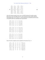
From the three nodal FBDs and noting that the nodal force vector has six components, we
can easily arrive at the following six equilibrium equations expressed in matrix form:

1
2
3
1
2
3
1
2
1
2
3
2
1
3
3
P
y2
P
x2
(F
y2
)
1
+(F
y2
)
2
(F
x2
)

1
+
(F
x2
)
2
P
y3
P
x3
(F
y3
)
2
+(F
y3
)
3
(F
x3
)
2
+
(F
x3
)
3
P
y1
P

x1
(F
y1
)
1
+(F
y1
)
3
(F
x1
)
1
+
(F
x1
)
3
(F
y1
)
3
(F
x1
)
3
N
ODE 2 FBD
N
ODE 1 FBD

N
ODE 3 FBD
(F
x1
)
1
(F
y1
)
1
(F
x2
)
2
(F
x2
)
1
(F
y2
)
1
(F
y2
)
2
(F
x3
)
2

(F
y3
)
2
(F
x3
)
3
(F
y3
)
3
Truss Analysis: Matrix Displacement Method by S. T. Mau
15
P =
⎪
⎪
⎪
⎪
⎭
⎪
⎪
⎪
⎪
⎬
⎫
⎪
⎪
⎪
⎪

⎩
⎪
⎪
⎪
⎪
⎨
⎧
3
3
2
2
1
1
y
x
y
x
y
x
P
P
P
P
P
P
=
1
2
2
1

1
0
0
⎪
⎪
⎪
⎪
⎭
⎪
⎪
⎪
⎪
⎬
⎫
⎪
⎪
⎪
⎪
⎩
⎪
⎪
⎪
⎪
⎨
⎧
y
x
y
x
F

F
F
F
+
2
3
3
2
2
0
0
⎪
⎪
⎪
⎪
⎭
⎪
⎪
⎪
⎪
⎬
⎫
⎪
⎪
⎪
⎪
⎩
⎪
⎪
⎪

⎪
⎨
⎧
y
x
y
x
F
F
F
F
+
3
3
3
1
1
0
0
⎪
⎪
⎪
⎪
⎭
⎪
⎪
⎪
⎪
⎬
⎫

⎪
⎪
⎪
⎪
⎩
⎪
⎪
⎪
⎪
⎨
⎧
y
x
y
x
F
F
F
F
(14)
where the subscript outside of each vector on the RHS indicates the member number.
Each of the vectors at the RHS, however, can be expressed in terms of their respective
nodal displacement vector using Eq.12, with the nodal forces and displacements referring
to the global nodal force and displacement representation:
⎪
⎪
⎭
⎪
⎪
⎬

⎫
⎪
⎪
⎩
⎪
⎪
⎨
⎧
2
2
1
1
y
x
y
x
F
F
F
F
=
1
44434241
34333231
24232221
14131211
⎥
⎥
⎥
⎥

⎦
⎤
⎢
⎢
⎢
⎢
⎣
⎡
kkkk
kkkk
kkkk
kkkk
⎪
⎪
⎭
⎪
⎪
⎬
⎫
⎪
⎪
⎩
⎪
⎪
⎨
⎧
2
2
1
1

v
u
v
u
⎪
⎪
⎭
⎪
⎪
⎬
⎫
⎪
⎪
⎩
⎪
⎪
⎨
⎧
3
3
2
2
y
x
y
x
F
F
F
F

=
2
44434241
34333231
24232221
14131211
⎥
⎥
⎥
⎥
⎦
⎤
⎢
⎢
⎢
⎢
⎣
⎡
kkkk
kkkk
kkkk
kkkk
⎪
⎪
⎭
⎪
⎪
⎬
⎫
⎪

⎪
⎩
⎪
⎪
⎨
⎧
3
3
2
2
v
u
v
u
⎪
⎪
⎭
⎪
⎪
⎬
⎫
⎪
⎪
⎩
⎪
⎪
⎨
⎧
3
3

1
1
y
x
y
x
F
F
F
F
=
3
44434241
34333231
24232221
14131211
⎥
⎥
⎥
⎥
⎦
⎤
⎢
⎢
⎢
⎢
⎣
⎡
kkkk
kkkk

kkkk
kkkk
⎪
⎪
⎭
⎪
⎪
⎬
⎫
⎪
⎪
⎩
⎪
⎪
⎨
⎧
3
3
1
1
v
u
v
u
Each of the above equations can be expanded to fit the form of Eq. 14:
1
2
2
1
1

0
0
⎪
⎪
⎪
⎪
⎭
⎪
⎪
⎪
⎪
⎬
⎫
⎪
⎪
⎪
⎪
⎩
⎪
⎪
⎪
⎪
⎨
⎧
y
x
y
x
F
F

F
F
=
1
44434241
34333231
24232221
14131211
000000
000000
00
00
00
00
⎥
⎥
⎥
⎥
⎥
⎥
⎥
⎥
⎦
⎤
⎢
⎢
⎢
⎢
⎢
⎢

⎢
⎢
⎣
⎡
kkkk
kkkk
kkkk
kkkk
⎪
⎪
⎪
⎪
⎭
⎪
⎪
⎪
⎪
⎬
⎫
⎪
⎪
⎪
⎪
⎩
⎪
⎪
⎪
⎪
⎨
⎧

3
3
2
2
1
1
v
u
v
u
v
u
Truss Analysis: Matrix Displacement Method by S. T. Mau
16
2
3
3
2
2
0
0
⎪
⎪
⎪
⎪
⎭
⎪
⎪
⎪
⎪

⎬
⎫
⎪
⎪
⎪
⎪
⎩
⎪
⎪
⎪
⎪
⎨
⎧
y
x
y
x
F
F
F
F
=
2
44434241
34333231
24232221
14131211
00
00
00

00
000000
000000
⎥
⎥
⎥
⎥
⎥
⎥
⎥
⎥
⎦
⎤
⎢
⎢
⎢
⎢
⎢
⎢
⎢
⎢
⎣
⎡
kkkk
kkkk
kkkk
kkkk
⎪
⎪
⎪

⎪
⎭
⎪
⎪
⎪
⎪
⎬
⎫
⎪
⎪
⎪
⎪
⎩
⎪
⎪
⎪
⎪
⎨
⎧
3
3
2
2
1
1
v
u
v
u
v

u
3
3
3
1
1
0
0
⎪
⎪
⎪
⎪
⎭
⎪
⎪
⎪
⎪
⎬
⎫
⎪
⎪
⎪
⎪
⎩
⎪
⎪
⎪
⎪
⎨
⎧

y
x
y
x
F
F
F
F
=
3
44434241
34333231
24232221
14131211
00
00
000000
000000
00
00
⎥
⎥
⎥
⎥
⎥
⎥
⎥
⎥
⎦
⎤

⎢
⎢
⎢
⎢
⎢
⎢
⎢
⎢
⎣
⎡
kkkk
kkkk
kkkk
kkkk
⎪
⎪
⎪
⎪
⎭
⎪
⎪
⎪
⎪
⎬
⎫
⎪
⎪
⎪
⎪
⎩

⎪
⎪
⎪
⎪
⎨
⎧
3
3
2
2
1
1
v
u
v
u
v
u
When each of the RHS vectors in Eq. 14 is replaced by the RHS of the above three
equations, the resulting equation is the unconstrained global stiffness equation:
⎥
⎥
⎥
⎥
⎥
⎥
⎥
⎥
⎦
⎤

⎢
⎢
⎢
⎢
⎢
⎢
⎢
⎢
⎣
⎡
666564636261
565554535251
464544434241
363534333231
262524232221
161514131211
KKKKKK
KKKKKK
KKKKKK
KKKKKK
KKKKKK
KKKKKK
⎪
⎪
⎪
⎪
⎭
⎪
⎪
⎪

⎪
⎬
⎫
⎪
⎪
⎪
⎪
⎩
⎪
⎪
⎪
⎪
⎨
⎧
3
3
2
2
1
1
v
u
v
u
v
u
=
⎪
⎪
⎪

⎪
⎭
⎪
⎪
⎪
⎪
⎬
⎫
⎪
⎪
⎪
⎪
⎩
⎪
⎪
⎪
⎪
⎨
⎧
3
3
2
2
1
1
y
x
y
x
y

x
P
P
P
P
P
P
(15)
where the components of the unconstrained global stiffness matrix, K
ij
, is the
superposition of the corresponding components in each of the three expanded stiffness
matrices in the equations above.
In actual computation, it is not necessary to expand the stiffness equation in Eq. 12 into
the 6-equation form as we did earlier. That was necessary only for the understanding of
how the results are derived. We can use the local-to-global DOF relationship in the
global DOF table and place the member stiffness components directly into the global
stiffness matrix. For example, component (1,3) of the member-2 stiffness matrix is added
to component (3,5) of the global stiffness matrix. This simple way of assembling the
global stiffness matrix is called the Direct Stiffness Method.
To carry out the above procedures numerically, we need to use the dimension and
member property given at the beginning of this section to arrive at the stiffness matrix for
each of the three members:
Truss Analysis: Matrix Displacement Method by S. T. Mau
17
(k
G
)
1
=(

1
22
22
22
22
1
)
⎥
⎥
⎥
⎥
⎥
⎦
⎤
⎢
⎢
⎢
⎢
⎢
⎣
⎡
−−
−−
−−
−−
SCSSCS
CSCCSC
SCSSCS
CSCCSC
L

EA
=
⎥
⎥
⎥
⎥
⎦
⎤
⎢
⎢
⎢
⎢
⎣
⎡
−−
−−
−−
−−
8.126.98.126.9
6.92.76.92.7
8.126.98.126.9
6.92.76.92.7
(k
G
)
2
=(
2
22
22

22
22
2
)
⎥
⎥
⎥
⎥
⎥
⎦
⎤
⎢
⎢
⎢
⎢
⎢
⎣
⎡
−−
−−
−−
−−
SCSSCS
CSCCSC
SCSSCS
CSCCSC
L
EA
=
⎥

⎥
⎥
⎥
⎦
⎤
⎢
⎢
⎢
⎢
⎣
⎡
−−
−−−
−−−
−−
8.126.98.126.9
6.92.76.92.7
8.126.98.126.9
6.92.76.92.7
(k
G
)
3
=(
3
22
22
22
22
3

)
⎥
⎥
⎥
⎥
⎥
⎦
⎤
⎢
⎢
⎢
⎢
⎢
⎣
⎡
−−
−−
−−
−−
SCSSCS
CSCCSC
SCSSCS
CSCCSC
L
EA
=
⎥
⎥
⎥
⎥

⎦
⎤
⎢
⎢
⎢
⎢
⎣
⎡
−
−
06.900
07.1607.16
0000
07.1607.16
When the three member stiffness matrices are assembled according to the Direct Stiffness
Method, the unconstrained global stiffness equation given at the beginning of this section
is obtained. For example, the unconstrained global stiffness matrix component k
34
is the
superposition of (k
34
)
1
of member 1 and (k
12
)
2
of member 2. Note that the unconstrained
global stiffness matrix has the same features as the member stiffness matrix: symmetric
and singular, etc.

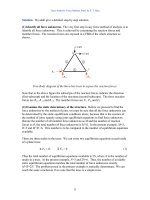
5. Constrained Global Stiffness Equation and Its Solution
Example 2. Now consider the same three-bar truss as shown before with E=70 GPa,
A=1,430 mm
2
for each member but with the support and loading conditions added.
A constrained and loaded truss in a global coordinate system.
x
y
1
2
4m
3m
2m
2m
3
3m
1
2
3
1.0 MN
0.5 MN
Truss Analysis: Matrix Displacement Method by S. T. Mau
18
Solution. The support conditions are: u
1
=0, v
1
=0, and v
3
=0. The loading conditions are:

P
x2
=0.5 MN, P
y2
= −1.0 MN, and P
x3
=0. The stiffness equation given at the beginning of
the last section now becomes
⎥
⎥
⎥
⎥
⎥
⎥
⎥
⎥
⎦
⎤
⎢
⎢
⎢
⎢
⎢
⎢
⎢
⎢
⎣
⎡
−−
−−

−−−
−−−
−−
−−−
8.126.98.126.900
6.199.236.92.706.16
8.126.96.2508.126.9
6.92.704.146.92.7
008.126.98.126.9
06.166.92.76.99.23
⎪
⎪
⎪
⎪
⎭
⎪
⎪
⎪
⎪
⎬
⎫
⎪
⎪
⎪
⎪
⎩
⎪
⎪
⎪
⎪

⎨
⎧
0
0
0
3
2
2
u
v
u
=
⎪
⎪
⎪
⎪
⎭
⎪
⎪
⎪
⎪
⎬
⎫
⎪
⎪
⎪
⎪
⎩
⎪
⎪

⎪
⎪
⎨
⎧
−
3
1
1
0
0.1
5.0
y
y
x
P
P
P
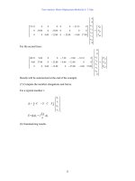
Note that there are exactly six unknown in the six equations. The solution of the six
unknowns is obtained in two steps. In the first step, we notice that the three equations, 3
rd
through 5
th
, are independent from the other three and can be dealt with separately.
⎥
⎥
⎥
⎦
⎤
⎢
⎢

⎢
⎣
⎡
−
−
9.236.92.7
6.96.250
2.704.14
⎪
⎭
⎪
⎬
⎫
⎪
⎩
⎪
⎨
⎧
3
2
2
u
v
u
=
⎪
⎭
⎪
⎬
⎫

⎪
⎩
⎪
⎨
⎧
−
0
0.1
5.0
(16)
Eq. 16 is the constrained stiffness equation of the loaded truss. The constrained 3x3
stiffness matrix is symmetric but not singular. The solution of Eq. 16 is: u
2
=0.053 m,
v
2
= −0.053 m, and u
3
= 0.037 m. In the second step, the reactions are obtained from the
direct substitution of the displacement values into the other three equations, 1
st
, 2
nd
and
6
th
:
⎥
⎥
⎥

⎦
⎤
⎢
⎢
⎢
⎣
⎡
−−
−−
−−−
8.126.98.126.900
008.126.98.126.9
06.166.92.76.99.23
⎪
⎪
⎪
⎪
⎭
⎪
⎪
⎪
⎪
⎬
⎫
⎪
⎪
⎪
⎪
⎩
⎪

⎪
⎪
⎪
⎨
⎧
−
0
037.0
053.0
053.0
0
0
=
⎪
⎭
⎪
⎬
⎫
⎪
⎩
⎪
⎨
⎧
−
83.0
17.0
5.0
=
⎪
⎭

⎪
⎬
⎫
⎪
⎩
⎪
⎨
⎧
3
1
1
y
y
x
P
P
P
or
⎪
⎭
⎪
⎬
⎫
⎪
⎩
⎪
⎨
⎧
3
1

1
y
y
x
P
P
P
=
⎪
⎭
⎪
⎬
⎫
⎪
⎩
⎪
⎨
⎧
−
83.0
16.0
5.0
MN
The member deformation represented by the member elongation can be computed by the
member deformation equation, Eq. 3:
Truss Analysis: Matrix Displacement Method by S. T. Mau
19
Member 1:
∆
1

=
⎣⎦
1
SCSC −−
⎪
⎪
⎭
⎪
⎪
⎬
⎫
⎪
⎪
⎩
⎪
⎪
⎨
⎧
2
2
1
1
v
u
v
u
=
⎣⎦
1
8.06.08.06.0 −−

⎪
⎪
⎭
⎪
⎪
⎬
⎫
⎪
⎪
⎩
⎪
⎪
⎨
⎧
− 053.0
053.0
0
0
= -0.011m
For member 2 and member 3, the elongations are
∆
2
= −0.052m, and
∆
3
=0.037m.
The member forces are computed using Eq. 1.
F=k
∆
=

L
EA
∆
F
1
= −0.20 MN, F
2
= −1.04 MN, F
3
= 0.62 MN
The results are summarized in the following table.
Nodal and Member Solutions
Displacement (m) Force (MN)
Node
x-direction y-direction x-direction y-direction
1 0 0 -0.50 0.16
2 0.053 -0.053 0.50 -1.00
3 0.037 0 0 0.83
Member Elongation (m) Force (MN)
1 -0.011 -0.20
2 -0.052 -1.04
3 0.037 0.62
Problem 2. Consider the same three-bar truss as that in Example 2, but with a different
numbering system for members. Construct the constrained stiffness equation, Eq. 16.
Problem 2.
x
y
1
2
4m

3m
2m
2m
3
3m
1
3
2
1.0 MN
0.5 MN