Numerical Solution of Differential Algebraic Equations

IMM
DEPARTMENT OF MATHEMATICAL MODELLING
Technical University of Denmark
DK-2800
Lyngby – Denmark

May 6, 1999
CBE

Numerical Solution of
Differential Algebraic
Equations

Editors: Claus Bendtsen
Per Grove Thomsen
TECHNICAL REPORT
IMM-REP-1999-8

IMM



Contents
Preface

v

Chapter 1. Introduction
1.1. Definitions
1.1.1. Semi explicit DAEs
1.1.2. Index

1.1.2.1. Singular algebraic constraint
1.1.2.2. Implicit algebraic variable
1.1.3. Index reduction
1.2. Singular Perturbations
1.2.1. An example
1.3. The Van der Pol equation

1
1
2
2
2
2
4
5
5
5

Part 1. Methods

7

Chapter 2. Runge-Kutta Methods for DAE problems
2.1. Introduction
2.1.1. Basic Runge-Kutta methods
2.1.2. Simplifying conditions
2.1.3. Order reduction, stage order, stiff accuracy
2.1.4. Collocation methods
2.2. Runge-Kutta Methods for Problems of Index 1
2.2.1. State Space Form Method

2.2.2. The ε-embedding method for problems of index 1
2.3. Runge-Kutta Methods for high-index problems
2.3.1. The semi-explicit index-2 system
2.3.2. The ε-embedding method
2.3.3. Collocation methods
2.3.4. Order-table for some methods in the index-2 case
2.4. Special Runge-Kutta methods
2.4.1. Explicit Runge-Kutta methods (ERK)
i

9
9
9
10
10
11
11
12
12
14
14
14
15
16
16
16


2.4.2. Fully implicit Runge-Kutta methods (FIRK)
2.4.3. Diagonally Implicit Runge-Kutta methods (DIRK)

2.4.4. Design Criteria for Runge-Kutta methods
2.5. ε-Expansion of the Smooth Solution

17
17
18
18

Chapter 3. Projection Methods
3.1. Introduction
3.1.1. Problem
3.1.2. Example case
3.2. Index reduction
3.2.1. Example on index reduction
3.2.2. Restriction to manifold
3.2.3. Implications of reduction
3.2.4. Drift-off phenomenon
3.2.5. Example of drift-off
3.3. Projection
3.3.1. Coordinate projection
3.3.2. Another projection method and the projected RK method
3.4. Special topics
3.4.1. Systems with invariants
3.4.2. Over determined systems

23
23
23
23
24

24
26
27
27
27
29
29
30
31
31
31

Chapter 4. BDF-methods
4.1. Multi Step-Methods in general and BDF-methods
4.1.1. BDF-methods
4.2. BDF-methods applied to DAEs
4.2.1. Semi-Explicit Index-1 Systems
4.2.2. Fully-Implicit Index-1 Systems
4.2.3. Semi-Explicit Index-2 Systems
4.2.4. Index-3 Systems of Hessenberg form
4.2.5. Summary
4.2.6. DAE-codes

33
33
33
35
36
36
37

37
38
38

Chapter 5. Stabilized Multi-step Methods Using β-Blocking
5.1. Adams methods
5.2. β-blocking
5.2.1. Why β-blocking
5.2.2. Difference correcting
5.3. Consequences of β-blocking
5.4. Discretization of the Euler-Lagrange DAE Formulation

39
39
39
40
40
41
41

ii


5.4.1. Commutative application of the DCBDF method
5.4.2. Example: The Trapezoidal Rule
5.5. Observed relative error

42
43
44

Part 2. Special Issues

45

Chapter 6. Algebraic Stability
6.1. General linear stability - AN-stability
6.2. Non-linear stability

47
47
50

Chapter 7. Singularities in DEs
7.1. Motivation
7.2. Description of the method
7.3. Detailed description of the method
7.3.1. Singularities in ODEs
7.3.2. Projection: A little more on charts
7.3.3. Singularities in DAEs
7.3.4. Augmention: Making the singular ODE a nonsingular ODE
7.4. Implementing the algorithm

53
53
54
55
55
56
56

57
59

Chapter 8. ODEs with invariants
8.1. Examples of systems with invariants
8.2. Solving ODEs with invariants
8.2.1. Methods preserving invariants
8.2.2. Reformulation as a DAE
8.2.3. Stabilization of the ODE system
8.3. Flying to the moon
8.3.1. Going nowhere
8.3.2. Round about the Earth
8.3.3. Lunar landing
8.3.4. What’s out there?
8.4. Comments on Improvement of the Solution

63
63
64
64
64
64
65
67
68
69
70
70

Part 3. Applications

73

Chapter 9. Multibody Systems
9.1. What is a Multibody System?
9.2. Why this interest in Multibody Systems?
9.3. A little bit of history repeating
9.4. The tasks in multibody system analysis
9.5. Example of a multibody system

75
75
76
76
77
79

iii


9.5.1. The multibody truck
9.5.2. The pendulum
9.5.3. Numerical solution
9.6. Problems
9.7. Multibody Software

79
81
83
83

84

Chapter 10. DAEs in Energy System Models
10.1. Models of Energy System Dynamics
10.2. Example Simulations with DNA
10.2.1. Numerical methods of DNA
10.2.2. Example 1: Air flowing through a pipe
10.2.3. Example 2: Steam temperature control

85
85
87
87
90
91

Bibliography

97

Index

99

iv


Preface
These lecture notes have been written as part of a Ph.D. course on the numerical solution of Differential Algebraic Equations. The course was held at IMM
in the fall of 1998. The authors of the different chapters have all taken part in the

course and the chapters are written as part of their contribution to the course.
We hope that coming courses in the Numerical Solution of DAE’s will benefit
from the publication of these lecture notes.
The students participating is the course along with the chapters they have
written are as follows:
¯ Astrid Jørdis Kuijers, Chapter 4 and 5 and Section 1.2.1.
¯ Anton Antonov AntonovChapter 2 and 6.
¯ Brian ElmegaardChapter 8 and 10.
¯ Mikael Zebbelin PoulsenChapter 2 and 3.
¯ Falko Jens WagnerChapter 3 and 9.
¯ Erik Østergaard, Chapter 5 and 7.

v


vi

PREFACE


CHAPTER 1

Introduction
The (modern) theory of numerical solution of ordinary differential equations
(ODEs) has been developed since the early part of this century – beginning with
Adams, Runge and Kutta. At the present time the theory is well understood
and the development of software has reached a state where robust methods are
available for a large variety of problems. The theory for Differential Algebraic
Equations (DAEs) has not been studied to the same extent – it appeared from
early attempts by Gear and Petzold in the early 1970’es that not only are the

problems harder to solve but the theory is also harder to understand.
The problems that lead to DAEs are found in many applications of which
some are mentioned in the following chapters of these lecture notes. The choice
of sources for problems have been influenced by the students following this first
time appearance of the course.
1.1. Definitions
The problems considered are in the most general form a fully implicit equation of the form
(1.1)

F´y¼ yµ

0

where F and y are of dimension n and F is assumed to be sufficiently smooth.
This is the autonomous form, a non-autonomous case is defined by
F´x y¼ yµ

0

Notice that the non-autonomous equation may be made autonomous by adding
the equation x¼ 1 and we do therefore not need to consider the non-autonomous
form seperately1 .
A special case arises when we can solve for the y¼ -variable since we (at least
formally) can make the equation explicit in this case and obtain a system of
∂F
ODEs. The condition to be fullfilled is that ∂y
¼ is nonsingular. When this is not
the case the system is commonly known as being differential algebraic and this
1 this

may be subject to debate since the non-autonomous case can have special features
1


2

1. INTRODUCTION

will be the topic of these notes. In order to emphasize that the DAE has the
general form Eq. 1.1 it is normally called a fully implicit DAE. If F in addition
is linear in y (and y¼ ) (i.e. has the form A´xµy · B´xµy¼ 0) the DAE is called
linear and if the matrices A and B further more are constant we have a constant
coefficient linear DAE.
1.1.1. Semi explicit DAEs. The simplest form of problem is the one where
we can write the system in the form
(1.2)

y¼

f´y zµ

0

g´y zµ

and gz (the partial derivative ∂g ∂z) has a bounded inverse in a neighbourhood
of the solution.
Assuming we have a set of consistent initial values ´y0 z0 µ it follows from
the inverse function theorem that z can be found as a function of y. Thus local existence, uniqueness and regularity of the solution follows from the conventional
theory of ODEs.

1.1.2. Index. Numerous examples exist where the conditions above do not
hold. These cases have general interest and below we give a couple of examples
from applications.
1.1.2.1. Singular algebraic constraint. We consider the problem defined by
the system of three equations
y¼1
0
0

y3

y2 ´1   y2 µ

y1 y2 · y3 ´1   y2µ   x

where x is a parameter of our choice. The second equation has two solutions
y2 0 and y2 1 and we may get different situations depending on the choice
of initial conditions:
1. if y2 0 we get y3 x from the last equation and we can solve the first
equation for y1 .
2. Setting y2 1 we get y1 x from the last equation and y3 1 follows
from the first equation.
1.1.2.2. Implicit algebraic variable.
(1.3)

y¼
0

f ´y z µ
g´yµ

1.1. DEFINITIONS

3

In this case we have that gz 0 and the condition of boundedness of the inverse
does not hold. However if gy fz has a bounded inverse we can do the trick of
differentiating the second equation leading to system
y¼

f ´y zµ

0

gy ´yµ f ´y zµ

and this can then be treated like the semi explicit case, Eq. 1.2. This motivates
the introduction of index.
D EFINITION 1.1 (Differential index). For general DAE-systems we define
the index along the solution path as the minimum number of differentiations
of the systems, Eq. 1.1 that is required to reduce the system to a set of ODEs for
the variable y.
The concept of index has been introduced in order to quantify the level of
difficulty that is involved in solving a given DAE. It must be stressed, as we indeed will see later, that numerical methods applicable (i.e. convergent) for DAEs
of a given index, might not be useful for DAEs of higher index.
Complementary to the differential index one can define the pertubation index
[HLR89].
D EFINITION 1.2 (Perturbation index). Eq. 1.1 is said to have perturbation
index m along a solution y if m is the smallest integer such that, for all functions

yˆ having a defect
F´yˆ ¼ yˆ µ

δ´xµ

there exists an estimate
yˆ ´xµ   y´xµ

C´ yˆ ´0µ   y´0µ

· max

δ´ξµ

·
· max

δ´m 1µ´ξµ

µ

whenever the expression on the right hand side is sufficiently small. C is a constant that depends only on the function F and the length of the interval.
If we consider the ODE-case Eq. 1.1, the lemma by Gronwall (see [HNW93,
page 62]) gives the bound
(1.4)

yˆ´xµ   y´xµ

C´ yˆ´0µ   y´0µ

·

ξ

max

0 ξ x

0

δ´t µdt

µ

If we interpret this in order to find the perturbation index it is obviously zero.


4

1. INTRODUCTION

1.1.3. Index reduction. A process called index reduction may be applied to
a system for lowering the index from an initially high value down to e.g. index
one. This reduction is performed by successive differentiation and is often used
in theoretical contexts. Let us illustrate it by an example:
We look at example 1.1.2.2 and differentiate Eq. 1.3 once, thereby obtaining
y¼

f ´y zµ

0

gy ´yµ f ´y zµ

Differentiating Eq. 1.3 once more leads to
y¼

0

f ´y zµ

gyy ´yµ´ f ´y zµµ2 · gy ´yµ´ fy ´y zµ f ´y zµ · fz ´y zµz¼ µ

which by rearranging terms can be expressed as
y¼

f ´y zµ

z¼

  gyy ´yµ´ f ´y zgµµ´y·µ fgy´´yyµzµfy´y zµ f ´y zµ

2

y

z

The two differentiations have reduced the system to one of index zero and we
can solve the resulting ODE-system using well known methods.

If we want to find the perturbation index we may look at the equations for
the perturbed system
yˆ¼

f ´yˆ zˆµ · δ´xµ

0

g´yˆµ · θ´xµ

Using differentiation on the second equation leads to
0

gy ´yˆµ f ´yˆ zˆµ · gy ´yˆµδ´xµ · θ¼´xµ

From the estimates above we can now (by using Gronwalls lemma Eq. 1.4) obtain
yˆ´xµ   y´xµ

C´ yˆ´0µ   y´0µ
x

0

zˆ´xµ   z´xµ

´

δ´ξµ

·

·

θ¼´ξµ µdξ

C´ yˆ´0µ   y´0µ

·

max δ´ξµ · max θ¼ ´ξµ

All the max- values are to be taken over 0

ξ

x.

µ


1.3. THE VAN DER POL EQUATION

5

1.2. Singular Perturbations
One important source for DAE-problems comes from using singular perturbations [RO88] Here we look at systems of the form
y¼

εz¼

(1.5)

f´y zµ
ε

g´y zµ where 0

1

Letting ε go to zero (ε
0) we obtain an index one problem in semi-explicit
form. This system may be proven to have an ε-expansion where the expansion
coefficients are solution to the system of DAEs that we get in the limit of Eq. 1.5.
1.2.1. An example. In order to show the complex relationship between singular pertubation problems and higher index DAEs, we study the following problem:
y¼

f1 ´x y z εµ

y0

ζ0

εz¼

f2 ´x y z εµ

z0

g´0 ζ0 εµ
ε

where ε

1

which can be related to the reduced problem (by letting ε
y¼

f1 ´x y z 0µ

0

f2 ´x y z 0µ

0)

This is a DAE-system in semi-explicit form and we can differentiate the second
equation with respect to x and obtain
0

y¯ ¼ f1 ´x y¯ z¯ 0µ
gy ´x y¯ 0µf2 ´x y¯ z¯ 0µ · gx ´x y¯ 0µ

y¯0

ζ0

This shows, that for indexes greater than one the DAE and the stiff problem can
not always be related easily.
Singular Pertubation Problems (SPP) are treated in more detail in Subsection

2.2.2.
1.3. The Van der Pol equation
A very famous test problem for systems of ODEs is the Van der Pol equation
defined by the second order differential equation
y¼¼

µ´1   y2 µy¼   y


6

1. INTRODUCTION

This equation may be treated in different ways, the most straigtforward is to
split the equation into two by introducing a new variable for the derivative (y1
y y2 y¼ ) which leads to
y1 ¼
y2 ¼

y2

µ´1   y12 µy2   y1

The system of two ODEs may be solved by any standard library solver but the
outcome will depend on the solver and on the parameter µ. If we divide the second of the equations by µ we get an equation that has the character of a singular
perturbation problem. Letting µ
∞ we see that this corresponds to ε
0 in
Eq. 1.5.
Several other approaches may show other aspects of the nature of this problem for example [HW91] introduces the transformation t x µ after a scaling of

y2 by µ we get
y¼1

y2

y¼

µ2 ´´1   y12 µy2   y1 µ

2

The introduction of ε
form

1 µ2 finally results in a problem in singular perturbation
y¼1

y2

2

´1

εy¼

  y12µy2   y1

As explained previously this problem will approach a DAE if ε 0 Using terminology from ODEs the stiffness of the problem increases as ε gets smaller giving
rise to stability problems for numerical ODE-solvers that are explicit while we
expect methods that are A- or L-stable to perform better.

Part 1

Methods



CHAPTER 2

Runge-Kutta Methods for DAE problems
Written by Anton Antonov Antonov & Mikael Zebbelin Poulsen
Keywords: Runge-Kutta methods, order reduction phenomenon,
stage order, stiff accuracy, singular perturbation problem, index-1
and index-2 systems, ε-embedding, state space method, ε-expansion, FIRK and DIRK methods.
2.1. Introduction
Runge-Kutta methods have the advantage of being one-step methods, possibly having high order and good stability properties, and therefore they (and
related methods) are quite popular.
When solving DAE systems using Runge-Kutta methods, the problem of
incorporation of the algebraic equations into the method exists. This chapter
focuses on understanding algorithms and convergence results for Runge-Kutta
methods. The specific Runge-Kutta tables (i.e. coefficients) has to be looked up
elsewhere, eg. [HW96], [AP98] or [ESF98].
2.1.1. Basic Runge-Kutta methods. To settle notation we recapitulate the
form of the s-stage Runge-Kutta method.
For the autonomous explicit ODE system
y¼

f´yµ

the method, for advancing the solution from a point yn to the next, would look
like this:
s

(2.1a)

Yn i

yn · h ∑ ai j f´Yn

jµ

i

12

s

j 1
s

(2.1b)

yn·1

yn · h ∑ bi f´Yn iµ
i 1

The method is a one-step method (i.e. it does not utilize information from previous steps) and it is specified by the matrix A with the elements ai j , and the
9

10

2. RUNGE-KUTTA METHODS FOR DAE PROBLEMS

vector b having the elements bi . We call the Yn i’s the internal stages of the step.
In general these equations represents a non-linear system of equations.
The classical theory for determining the order of the local and global error is
found in a number of books on ODEs. Both the J. C. Butcher and P. Albrecht
approach are shortly described in [Lam91].
2.1.2. Simplifying conditions. The construction of implicit Runge-Kutta
methods is often done with respect to some simplifying (order) conditions , see
[HW96, p.71]:
q 1

1
q

∑ ai j cqj  1

ci
q

i

1

bj
q

´1   c j µ
q

j

1

s

(2.2a)
(2.2b)
(2.2c)

B´ pµ :
C´ηµ :
D´ζµ :

∑ bici

i 1
s

j 1
s

q  1

∑ bici

i 1

ai j

q

1

p

s

q

1

η

s

q

1

ζ

q

Condition B´ pµ is the quadrature condition, and C´ηµ could be interpreted as the
quadrature condition for the internal stages. A theorem of Butcher now says
T HEOREM 2.1. If the coefficients bi , ci and ai j of a Runge-Kutta method

satisfies B´ pµ, C´ηµ and D´ζµ with p η · ζ and p 2η · 2, then the method is
of order p.
Comment: You could say “at least order p”, or - that to discover the properties
of the method, - try to find a p as high as possible.
2.1.3. Order reduction, stage order, stiff accuracy. When using an implicit Runge-Kutta method for solving a stiff system, the order of the error can
be reduced compared to what the classical theory predicts. This phenomenon is
called order reduction.
The cause of the classical order “failing”, is that the step size is actually “chosen” much to large compared to the time scale of the system. We know though,
and our error estimates often tells the same, that we get accurate solutions even
though choosing such big step-sizes. This has to do with the fact that in a stiff
system we are not following the solution curve, but we are actually following the
“stable manifold”
The order we observe is (at least) described by the concept of stage order.
The stage order is the minimum of p and q when the Runge-Kutta method
satisfies B´ pµ and C´qµ from Eq. 2.2.


2.2. RUNGE-KUTTA METHODS FOR PROBLEMS OF INDEX 1

11

A class of methods not suffering from order reduction are the methods which
are stiffly accurate. Stiff accuracy means that the final point is actually one of
the internal stages (typically the last stage), and therefore the method satisfies
bi

asi

i

1

s

2.1.4. Collocation methods. Collocation is a fundamental numerical method. It is about fitting a function to have some properties in some chosen collocation points. Normally the collocation function would be a polynomial P´xµ of
some degree r.
The collocation method for integrating a step (like Eq. 2.1a) would be to find
coefficients so that
P´xn µ yn
P¼ ´xn · ci hµ
yn·1

f´xn · ci h P´xn · ci hµµ

i

12

s

P´xn · hµ

Collocation methods are a relevant topic when discussing Runge-Kutta methods. It turns out that some special Runge-Kutta methods like Gauss, Radau IIA
and Lobatto IIIA, are in fact collocation methods.
In [Lam91, p. 194] it is shown why such a method is a Runge-Kutta method.
The principle is that the ci in the collocation formula matches the ones from the
Runge-Kutta method, and the internal stages of the Runge-Kutta method match
the collocation method as Yi P´xn · ci hµ. The “parameters” of the collocation
method are the ci ’s and therefore define the A-matrix of the identical (implicit)
Runge-Kutta method.

2.2. Runge-Kutta Methods for Problems of Index 1
The traditional form of the index-one problem looks like this:
(2.3a)
(2.3b)

y¼
0

f´y zµ
g´y zµ

with the assumption that
(2.3c)

gz ´y zµ is invertible

for every point at the solution curve. If gz ´y zµ were not invertible the system
would have index at least 2.
This implies that Eq. 2.3b has a unique solution z G´yµ by the Implicit
Function Theorem. Inserted into Eq. 2.3a gives
(2.4)

y¼

f´y G´yµµ


12

2. RUNGE-KUTTA METHODS FOR DAE PROBLEMS

- the so called state space form. We see that, if algebraic manipulations could
lead to Eq. 2.4, then we could solve the problem as a normal explicit ODE problem. This is in general not possible.
We should at this time mention another form of the implicit ODE system:
The form
My¼

f´yµ

typically occurs when you can’t separate differential and algebraic equations like
in Eq. 2.3, and some of the equations contain more than one “entry” of the primes
y¼i from y¼ , see eg. [HW96, p. 376 ff.].
If M is invertible/regular, this system is actually just a normal ODE system
(index-0), and traditional methods can be used. If M is singular the system has
index at least one.
If the system is of index-1 then a linear transformation of the variables can
give the system a form like Eq. 2.3.
2.2.1. State Space Form Method. Because of the possibility of (at least
“implicitly”) rewriting the problem to the state space form Eq. 2.4, we could
imagine using the Runge-Kutta method, by solving Eq. 2.3b (for z) in each of
the internal stages and at the final solution point:
s

Yn i

yn · h ∑ ai j f´Yn j Zn

jµ

j 1

0

i

12

s

g´Yn i Zn i µ
s

yn·1

yn · h ∑ bi f´Yn i Zn iµ
i 1

0

g´yn·1 zn·1 µ

These methods have the same order as the classical theory would predict for
Runge-Kutta methods with some A and b, and this holds for both y and z.
Furthermore these methods do not have to be implicit. The explicit state
space form methods are treated in [ESF98, p. 182], here called half-explicit
Runge-Kutta methods.
2.2.2. The ε-embedding method for problems of index 1. Discussions of
index-1 problems are often introduced by presenting the singular perturbation
problem (SPP) already encountered in Section 1.2. A key idea (see eg. [HW96, p.
374]) is the following: Transform the DAE to a SPP, by introducing ε. Deriving

the method for a SPP and then putting ε 0. This will give a method for DAE
of index 1:


2.2. RUNGE-KUTTA METHODS FOR PROBLEMS OF INDEX 1

13

s

(2.6a)
(2.6b)

yn · h ∑ ai j f´Yn j Zn

Yn i

jµ

i

12

s

i

12

s

j 1
s

εzn · h ∑ ai j g´Yn j Zn

εZn i

jµ

j 1

s

yn · h ∑ bi f´Yn i Zn i µ

yn·1

(2.6c)

i 1
s

εzn · h ∑ bi g´Yn i Zn i µ

εzn·1

(2.6d)

i 1

In order to eliminate ε from (2.6) we have
s

hg´Yn i Zn i µ

ε ∑ wi j ´Zn
j 1

j

  znµ

from Eq. 2.6b, where ωi j
ai j  1 . This means that A is invertible and
therefore the RK methods for ε-embedding must at least be implicit. So lets at
last put ε 0
s

(2.7a)

Yn i

yn · ∑ ai j f´Yn j Zn

jµ

i

12

s

i

12

s

j 1

(2.7b)

0

(2.7c)

yn·1

g´Yn i Zn iµ
s

yn · h ∑ bi f´Yn i Zn i µ
i 1
s

(2.7d)

zn·1

´1

s

  ∑ biωi j µzn · ∑ biωi j Zn j µ
j 1

i j 1

If we replace Eq. 2.7d with
(2.7e)

µ Zn j

0

g´yn·1 zn·1 µ

G´Yn j µ and zn·1 G´yn·1µ In this case Eq. 2.7 is identical to the
solution of the state space form with the same RK method. The same would hold
if the method were stiffly accurate. In these cases the error is predicted by the
classical order theory referred to previously.


14

2. RUNGE-KUTTA METHODS FOR DAE PROBLEMS

Generally the convergence results are listed in [HW96, p.380]. We should
though mention the convergence result if the method is not stiffly accurate, but

linearly stable at infinity: Then the method has the minimum of the classical
order and the stage order + 1.
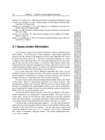
We have the following diagram:
ε

SPP

0

z=G(y)

DAE

ODE
RK

RK
Solution

ε

0

direct approach
indirect approch

Solution

F IGURE 2.1. The transformation of the index-1 problem
2.3. Runge-Kutta Methods for high-index problems

Not many convergence results exist for high-index DAEs.
2.3.1. The semi-explicit index-2 system. For problems of index 2, results
mainly exist for the semi-explicit index-2 problem. It looks as follows:
(2.8a)

y¼

f´y zµ

(2.8b)

0

g´yµ

with
gy ´yµf´y zµ being invertible.

(2.8c)

2.3.2. The ε-embedding method. This method also applies to the semiexplicit index-2 case, although in a slightly different form: (note that the new
variable ln j is introduced)
s

(2.9a)

Yn i

yn · h ∑ ai j f´Yn j Zn

jµ

i

12

s

i

12

s

i

12

s

j 1

(2.9b)

0

(2.9c)

Zn i

g´Yn iµ
s

zn · h ∑ ai j ln
j 1

j


2.3. RUNGE-KUTTA METHODS FOR HIGH-INDEX PROBLEMS

15

s

(2.9d)

yn · h ∑ bi f´Yn i Zn i µ

yn·1

i 1
s

(2.9e)

zn · h ∑ bi ln

zn·1

j

i 1

Convergence results are described in [HW96, p. 495 ff.]. The main convergence results are based on the simplifying conditions
B´ pµ and C´qµ
see Eq. 2.2. An abstract of convergence results are that the local error then
behaves like
LE ´yµ O ´hq·1µ

O ´hqµ

LE ´zµ
with p

q. The interesting result for the global error is then that

´

GE ´yµ

O ´hq·1µ
O ´hqµ

if p
if p

q
q

O ´hqµ

GE ´zµ

Remember that these results deal with the method used for the semi-explicit
index-2 problem. The convergence results are, as presented, concentrated useful
implications of more general results found in [HW96].
2.3.3. Collocation methods. The collocation method, matching an s-stage
Runge-Kutta method could be applied to Eq. 2.8, as follows: Let u´xµ and v´xµ
be polynomials of degree s. At some point xn the polynomial satisfies consistent
initial conditions
u´xn µ

(2.10a)

yn

v´xn µ

zn

Then the collocation polynomials are found to satisfy
(2.10b)

u¼ ´xn · ci hµ

0

µ

f´u´xn · ci hµ v´xn · ci hµµ
g´u´xn · ci hµµ

i

12

s

and the step is finally determined from
(2.10c)

yn·1

u´xn · hµ

zn·1

v´xn · hµ

It can be shown that this method coincides with the ε-method just mentioned,
if the coefficients are chosen correctly. The Gauss-, Radau IIA-, and Lobatto IIIA


16

2. RUNGE-KUTTA METHODS FOR DAE PROBLEMS

coefficients could therefore be used in both methods. These coefficients are quite
popular, when solving DAEs.

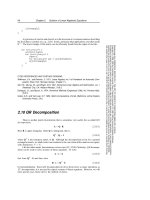
2.3.4. Order-table for some methods in the index-2 case. Here we present
a table with some of the order results from using the above methods.
Method
stages local error global error
y
z
y
z
s
·1
s
s
·1
s
 
Gauss
s odd h
h
h
h 1
s
·1
s
s
Gauss
s even h
h
h
hs 2
2s

·1
2s
projected Gauss
s
h
h
Radau IA
s
hs
hs 1
hs
hs 1
2s
 
1
2s
 
2
projected Radau IA
s
h
h
Radau IIA
s
h2s h2s 1 h2s 2 hs 1
Lobatto IIIA
s odd h2s 1
hs
h2s 2 hs 1
2s

 
1
s
Lobatto IIIA
s odd h
h
h2s 2
hs
2s
 
1
s
 
1
2s
 
2
Lobatto IIIC
s odd h
h
h
hs 1
For results on projection methods we refer to the chapter about Projection
methods, Chapter 3 or we refer to the text in [HW96, p.502].
2.4. Special Runge-Kutta methods
This section will give an overview of some special classes of methods. These
classes are defined by the structure of their coefficient matrix A. Figure 2.2 gives
an overview of these structures. The content is presented with inspiration from
[Kvæ92] and [KNO96].
2.4.1. Explicit Runge-Kutta methods (ERK). These methods have the

nice property that the internal stages one after one are expressed explicitly from
former stages. The typical structure of the A-matrix would the be
ai j

0

j

i

These methods are very interesting in the explicit ODE case, but looses importance when we introduce implicit ODEs. In this case the computation of the
internal stages would in general imply solving a system of nonlinear equations
for each stage, and introduce iterations. Additionally the stability properties of
these methods are quite poor.
As a measure of the work load we could use the factorization of the Jacobian.
We have an implicit n-dimensional ODE system. Since the factorization should
be done for each stage the work load for the factorization is of the order sn3 .


2.4. SPECIAL RUNGE-KUTTA METHODS

17

2.4.2. Fully implicit Runge-Kutta methods (FIRK). These methods have
no restriction on the elements of A. An s-stage FIRK method together with an
implicit ODE system, forms a fully implicit nonlinear equation system with a
number of equations in the order of ns. The work done in factorization of the
Jacobian would be of the order ´snµ3 s3 n3 .
2.4.3. Diagonally Implicit Runge-Kutta methods (DIRK). In order to
avoid the full Jacobian from the FIRK method, one could construct a semi explicit (close to explicit) method, by making the structure of A triangular and

thereby the Jacobian of the complete nonlinear equation system block-triangular. The condition of the A being triangular is traditionally expressed as
ai j

(2.11)

0

j

i

The work load could again be related to the factorization of the Jacobian. In each
stage we have n equations and the factorization would cost in the order of n3 per
stage. This means that the total workload would be of the order sn3 just as for
the ERK methods, when used on the implicit ODE system.
But as a major advantage these methods have better stability properties than
ERK methods. On the other hand they can not match the order of the FIRK
methods with the same number of stages.
As a subclass of the DIRK methods one should notice the singly DIRK
method (SDIRK methods) which on top of Eq. 2.11 specifies that
aii

γ

i

1

s

Yet another class of method is the ESDIRK methods which introduces the
start point as the first stage, and hereafter looks like the SDIRK method: the
method is defined by Eq. 2.11 and
a11
aii
0
11111
00000
00000
11111
00000
11111
00000
11111
00000
11111
ERK

11111
00000
00000
11111
00000
11111
00000
11111
00000
11111
FIRK

0
γ

i

2

11111
00000
0
00000
11111
00000
11111
00000
11111
00000
11111
DIRK

s
γ

γ
0
11111
00000
γ
00000
11111

γ
00000
11111
γ
00000
11111
00000
11111

SDIRK

0
111111
000000
γ
0
000000
111111
γ
000000
111111
γ
000000
111111
000000γ
111111

ESDIRK

F IGURE 2.2. Overview of the structure of A for the different

classes of methods