Tài liệu Solution of Linear Algebraic Equations part 4 docx
Bạn đang xem bản rút gọn của tài liệu. Xem và tải ngay bản đầy đủ của tài liệu tại đây (178.02 KB, 8 trang )
2.3 LU Decomposition and Its Applications
43
Sample page from NUMERICAL RECIPES IN C: THE ART OF SCIENTIFIC COMPUTING (ISBN 0-521-43108-5)
Copyright (C) 1988-1992 by Cambridge University Press.Programs Copyright (C) 1988-1992 by Numerical Recipes Software.
Permission is granted for internet users to make one paper copy for their own personal use. Further reproduction, or any copying of machine-
readable files (including this one) to any servercomputer, is strictly prohibited. To order Numerical Recipes books,diskettes, or CDROMs
visit website or call 1-800-872-7423 (North America only),or send email to (outside North America).
Isaacson, E., and Keller, H.B. 1966,
Analysis of Numerical Methods
(New York: Wiley),
§
2.1.
Johnson, L.W., and Riess, R.D. 1982,
Numerical Analysis
, 2nd ed. (Reading, MA: Addison-
Wesley),
§
2.2.1.
Westlake, J.R. 1968,
A Handbook of Numerical Matrix Inversion and Solution of Linear Equations
(New York: Wiley).
2.3 LU Decomposition and Its Applications
Suppose we are able to write the matrix A as a product of two matrices,
L · U = A (2.3.1)
where L is lower triangular (has elements only on the diagonal and below) and U
is upper triangular (has elements only on the diagonal and above). For the case of
a 4 × 4 matrix A, for example, equation (2.3.1) would look like this:
α
11
000
α
21
α
22
00
α
31
α
32
α
33
0
α
41
α
42
α
43
α
44
·
β
11
β
12
β
13
β
14
0 β
22
β
23
β
24
00β
33
β
34
000β
44
=
a
11
a
12
a
13
a
14
a
21
a
22
a
23
a
24
a
31
a
32
a
33
a
34
a
41
a
42
a
43
a
44
(2.3.2)
We can use a decomposition such as (2.3.1) to solve the linear set
A · x =(L·U)·x=L·(U·x)=b (2.3.3)
by first solving for the vector y such that
L · y = b (2.3.4)
and then solving
U · x = y (2.3.5)
What is the advantage of breaking up one linear set into two successive ones?
The advantage is that the solution of a triangular set of equations is quite trivial, as
we have already seen in §2.2 (equation 2.2.4). Thus, equation (2.3.4) can be solved
by forward substitution as follows,
y
1
=
b
1
α
11
y
i
=
1
α
ii
b
i
−
i−1
j=1
α
ij
y
j
i =2,3,...,N
(2.3.6)
while (2.3.5) can then be solved by backsubstitutionexactly as in equations (2.2.2)–
(2.2.4),
x
N
=
y
N
β
NN
x
i
=
1
β
ii
y
i
−
N
j=i+1
β
ij
x
j
i = N − 1,N −2,...,1
(2.3.7)
44
Chapter 2. Solution of Linear Algebraic Equations
Sample page from NUMERICAL RECIPES IN C: THE ART OF SCIENTIFIC COMPUTING (ISBN 0-521-43108-5)
Copyright (C) 1988-1992 by Cambridge University Press.Programs Copyright (C) 1988-1992 by Numerical Recipes Software.
Permission is granted for internet users to make one paper copy for their own personal use. Further reproduction, or any copying of machine-
readable files (including this one) to any servercomputer, is strictly prohibited. To order Numerical Recipes books,diskettes, or CDROMs
visit website or call 1-800-872-7423 (North America only),or send email to (outside North America).
Equations (2.3.6) and (2.3.7) total (for each right-hand side b) N
2
executions
of an inner loop containing one multiply and one add. If we have N right-hand
sides which are the unit column vectors (which is the case when we are inverting a
matrix), then taking into account the leading zeros reduces the total execution count
of (2.3.6) from
1
2
N
3
to
1
6
N
3
, while (2.3.7) is unchanged at
1
2
N
3
.
Notice that, once we have the LU decomposition of A, we can solve with as
many right-hand sides as we then care to, one at a time. This is a distinct advantage
over the methods of §2.1 and §2.2.
Performing the LU Decomposition
How then can we solve for L and U,givenA? First, we write out the
i, jth component of equation (2.3.1) or (2.3.2). That component always is a sum
beginning with
α
i1
β
1j
+ ···=a
ij
The number of terms in the sum depends, however, on whether i or j is the smaller
number. We have, in fact, the three cases,
i<j: α
i1
β
1j
+α
i2
β
2j
+···+α
ii
β
ij
= a
ij
(2.3.8)
i = j : α
i1
β
1j
+ α
i2
β
2j
+ ···+α
ii
β
jj
= a
ij
(2.3.9)
i>j: α
i1
β
1j
+α
i2
β
2j
+···+α
ij
β
jj
= a
ij
(2.3.10)
Equations (2.3.8)–(2.3.10) total N
2
equations for the N
2
+ N unknown α’s and
β’s (the diagonal being represented twice). Since the number of unknowns is greater
than the number of equations, we are invited to specify N of the unknowns arbitrarily
andthentry to solvefor the others. In fact, as we shall see, itisalways possibleto take
α
ii
≡ 1 i =1,...,N (2.3.11)
A surprising procedure, now, is Crout’s algorithm, which quite trivially solves
the set of N
2
+ N equations (2.3.8)–(2.3.11) for all the α’s and β’s by just arranging
the equations in a certain order! That order is as follows:
• Set α
ii
=1,i=1,...,N (equation 2.3.11).
• For each j =1,2,3,...,N do these two procedures: First, for i =
1, 2,...,j, use (2.3.8), (2.3.9), and (2.3.11) to solve for β
ij
, namely
β
ij
= a
ij
−
i−1
k=1
α
ik
β
kj
. (2.3.12)
(When i =1in 2.3.12 the summation term is taken to mean zero.) Second,
for i = j +1,j+2,...,N use (2.3.10) to solve for α
ij
, namely
α
ij
=
1
β
jj
a
ij
−
j−1
k=1
α
ik
β
kj
. (2.3.13)
Be sure to do both procedures before going on to the next j.
2.3 LU Decomposition and Its Applications
45
Sample page from NUMERICAL RECIPES IN C: THE ART OF SCIENTIFIC COMPUTING (ISBN 0-521-43108-5)
Copyright (C) 1988-1992 by Cambridge University Press.Programs Copyright (C) 1988-1992 by Numerical Recipes Software.
Permission is granted for internet users to make one paper copy for their own personal use. Further reproduction, or any copying of machine-
readable files (including this one) to any servercomputer, is strictly prohibited. To order Numerical Recipes books,diskettes, or CDROMs
visit website or call 1-800-872-7423 (North America only),or send email to (outside North America).
c
g
i
b
d
f
h
j
diagonal elements
subdiagonal elements
etc.
etc.
x
x
a
e
Figure 2.3.1. Crout’s algorithm for LU decomposition of a matrix. Elements of the original matrix are
modified in the order indicated by lower case letters: a, b, c, etc. Shaded boxes show the previously
modified elements that are used in modifying two typical elements, each indicated by an “x”.
If you work through a few iterations of the above procedure, you will see that
the α’s and β’s that occur on the right-hand side of equations (2.3.12) and (2.3.13)
are already determined by the time they are needed. You will also see that every a
ij
is used only once and never again. This means that the corresponding α
ij
or β
ij
can
be stored in the location that the a used to occupy: the decomposition is “in place.”
[The diagonal unity elements α
ii
(equation 2.3.11) are not stored at all.] In brief,
Crout’s method fills in the combined matrix of α’s and β’s,
β
11
β
12
β
13
β
14
α
21
β
22
β
23
β
24
α
31
α
32
β
33
β
34
α
41
α
42
α
43
β
44
(2.3.14)
by columns from left to right, and within each column from top to bottom (see
Figure 2.3.1).
What about pivoting? Pivoting (i.e., selection of a salubrious pivot element
for the division in equation 2.3.13) is absolutely essential for the stability of Crout’s
46
Chapter 2. Solution of Linear Algebraic Equations
Sample page from NUMERICAL RECIPES IN C: THE ART OF SCIENTIFIC COMPUTING (ISBN 0-521-43108-5)
Copyright (C) 1988-1992 by Cambridge University Press.Programs Copyright (C) 1988-1992 by Numerical Recipes Software.
Permission is granted for internet users to make one paper copy for their own personal use. Further reproduction, or any copying of machine-
readable files (including this one) to any servercomputer, is strictly prohibited. To order Numerical Recipes books,diskettes, or CDROMs
visit website or call 1-800-872-7423 (North America only),or send email to (outside North America).
method. Only partial pivoting (interchange of rows) can be implemented efficiently.
However this is enough to make the method stable. This means, incidentally, that
we don’t actually decompose the matrix A into LU form, but rather we decompose
a rowwise permutation of A. (If we keep track of what that permutation is, this
decomposition is just as useful as the original one would have been.)
Pivoting is slightly subtle in Crout’s algorithm. The key point to notice is that
equation (2.3.12) in the case of i = j (its final application) is exactly the same as
equation (2.3.13) except for the division in the latter equation; in both cases the
upper limit of the sum is k = j − 1(=i−1). This means that we don’t have to
commit ourselves as to whether the diagonal element β
jj
is the one that happens
to fall on the diagonal in the first instance, or whether one of the (undivided) α
ij
’s
below it in the column, i = j +1,...,N, is to be “promoted” to become the diagonal
β. This can be decided after all the candidates in the column are in hand. As you
should be able to guess by now, we will choose the largest one as the diagonal β
(pivot element), then do all the divisions by that element en masse.ThisisCrout’s
method with partial pivoting. Our implementation has one additional wrinkle: It
initially finds the largest element in each row, and subsequently (when it is looking
for the maximal pivot element) scales the comparison as if we had initially scaled all
the equations to make their maximum coefficient equal to unity; this is the implicit
pivoting mentioned in §2.1.
#include <math.h>
#include "nrutil.h"
#define TINY 1.0e-20; A small number.
void ludcmp(float **a, int n, int *indx, float *d)
Given a matrix
a[1..n][1..n]
, this routine replaces it by the LU decomposition of a rowwise
permutation of itself.
a
and
n
are input.
a
is output, arranged as in equation (2.3.14) above;
indx[1..n]
is an output vector that records the row permutation effected by the partial
pivoting;
d
is output as ±1 depending on whether the number of row interchanges was even
or odd, respectively. This routine is used in combination with
lubksb
to solve linear equations
or invert a matrix.
{
int i,imax,j,k;
float big,dum,sum,temp;
float *vv; vv stores the implicit scaling of each row.
vv=vector(1,n);
*d=1.0; No row interchanges yet.
for (i=1;i<=n;i++) { Loop over rows to get the implicit scaling informa-
tion.big=0.0;
for (j=1;j<=n;j++)
if ((temp=fabs(a[i][j])) > big) big=temp;
if (big == 0.0) nrerror("Singular matrix in routine ludcmp");
No nonzero largest element.
vv[i]=1.0/big; Save the scaling.
}
for (j=1;j<=n;j++) { This is the loop over columns of Crout’s method.
for (i=1;i<j;i++) { This is equation (2.3.12) except for i = j.
sum=a[i][j];
for (k=1;k<i;k++) sum -= a[i][k]*a[k][j];
a[i][j]=sum;
}
big=0.0; Initialize for the search for largest pivot element.
for (i=j;i<=n;i++) { This is i = j of equation (2.3.12) and i = j +1 ...N
of equation (2.3.13).sum=a[i][j];
for (k=1;k<j;k++)
2.3 LU Decomposition and Its Applications
47
Sample page from NUMERICAL RECIPES IN C: THE ART OF SCIENTIFIC COMPUTING (ISBN 0-521-43108-5)
Copyright (C) 1988-1992 by Cambridge University Press.Programs Copyright (C) 1988-1992 by Numerical Recipes Software.
Permission is granted for internet users to make one paper copy for their own personal use. Further reproduction, or any copying of machine-
readable files (including this one) to any servercomputer, is strictly prohibited. To order Numerical Recipes books,diskettes, or CDROMs
visit website or call 1-800-872-7423 (North America only),or send email to (outside North America).
sum -= a[i][k]*a[k][j];
a[i][j]=sum;
if ( (dum=vv[i]*fabs(sum)) >= big) {
Is the figure of merit for the pivot better than the best so far?
big=dum;
imax=i;
}
}
if (j != imax) { Do we need to interchange rows?
for (k=1;k<=n;k++) { Yes, do so...
dum=a[imax][k];
a[imax][k]=a[j][k];
a[j][k]=dum;
}
*d = -(*d); ...and change the parity of d.
vv[imax]=vv[j]; Also interchange the scale factor.
}
indx[j]=imax;
if (a[j][j] == 0.0) a[j][j]=TINY;
If the pivot element is zero the matrix is singular (at least to the precision of the
algorithm). For some applications on singular matrices, it is desirable to substitute
TINY for zero.
if (j != n) { Now, finally, divide by the pivot element.
dum=1.0/(a[j][j]);
for (i=j+1;i<=n;i++) a[i][j] *= dum;
}
} Go back for the next column in the reduction.
free_vector(vv,1,n);
}
Here is the routine for forward substitution and backsubstitution,implementing
equations (2.3.6) and (2.3.7).
void lubksb(float **a, int n, int *indx, float b[])
Solves the set of
n
linear equations A·X = B.Here
a[1..n][1..n]
is input, not as the matrix
A but rather as its LU decomposition, determined by the routine
ludcmp
.
indx[1..n]
is input
as the permutation vector returned by
ludcmp
.
b[1..n]
is input as the right-hand side vector
B, and returns with the solution vector X.
a
,
n
,and
indx
are not modified by this routine
and can be left in place for successive calls with different right-hand sides
b
. This routine takes
into account the possibility that
b
will begin with many zero elements, so it is efficient for use
in matrix inversion.
{
int i,ii=0,ip,j;
float sum;
for (i=1;i<=n;i++) { When ii is set to a positive value, it will become the
index of the first nonvanishing element of b.Wenow
do the forward substitution, equation (2.3.6). The
only new wrinkle is to unscramble the permutation
as we go.
ip=indx[i];
sum=b[ip];
b[ip]=b[i];
if (ii)
for (j=ii;j<=i-1;j++) sum -= a[i][j]*b[j];
else if (sum) ii=i; A nonzero element was encountered, so from now on we
will have to do the sums in the loop above.b[i]=sum;
}
for (i=n;i>=1;i--) { Now we do the backsubstitution, equation (2.3.7).
sum=b[i];
for (j=i+1;j<=n;j++) sum -= a[i][j]*b[j];
b[i]=sum/a[i][i]; Store a component of the solution vector X.
} All done!
}