Introduction to Confocal Microscopy and Image Analysis
Bạn đang xem bản rút gọn của tài liệu. Xem và tải ngay bản đầy đủ của tài liệu tại đây (4.12 MB, 50 trang )
BMS 524 - “Introduction to Confocal Microscopy and Image Analysis”
Beyond confocal microscopy:
modern 3-D imaging techniques:
Bartek Rajwa
Assistant Professor
Bindley Bioscience Center
Purdue University
West Lafayette, IN
This work is licensed under a Creative Commons Attribution-NonCommercial-ShareAlike 2.5 License.
Slide # 1
3-D methods based on nonlinear optical phenomena
Nonlinear optical phenomena are not part of our
everyday experience!
• In “classical” optics the optical properties of materials are
independent of the intensity of illumination
• If the illumination is sufficiently intense, the optical
properties may depend on the characteristics of light!
– Several novel 3-D microscopy techniques rely on non-linear optical
phenomena
– 2-p and multiphoton microscopy
– Higher harmonics microscopy (SGH, TTH)
– Coherent Anti-Stokes Raman scattering microscopy (CARS)
2
Linear polarization
Ut tensio sic vis
~Robert Hooke
+
-
d 2x
dx
m 2 + 2Γ + Ω 2 x − (ξ ( 2) x 2 + ξ (3) x 3 + ) = −eE (t )
dt
dt
Harmonic terms
Position of electron
varies in response to
the electric field E(t)
Anharmonic terms
1
P = ε 0 χ E0 exp(−iωt ) + c.c., where
2
Ne 2
1
χ=
ε 0 m Ω 2 − 2iΓω − ω 2
P – macroscopic polarization. This is a
measure of the response of the electron
density distribution to a static electric
field .
3
Origins of optical nonlinearity
d 2x
dx
2
( 2) 2
(3) 3
m 2 + 2Γ + Ω x − (ξ x + ξ x + ) = −eE (t )
dt
dt
• When the anharmonic terms are included there is no
longer an exact solution for the equation of motion.
• We can approximate the solution by expressing x as a
power series in E. Equivalently we can expand P:
(1)
P = ε 0 (χ E + χ
( 2)
2
E +χ
( 3)
3
E +χ
( 4)
4
E )
4
Some examples of nonlinear phenomena
• 1st order (linear) process: absorption and
reflection
• 2nd order process: SHG, Pockels effect
• 3rd order process: 2-photon absorption,
Kerr effect, CARS
• 2m-1 order: m-photon absorption
5
What is multiphoton (two photon) excitation?
• MPE of molecules is a nonlinear process involving
the absorption of multiple photons whose combined
energy is sufficient to induce a molecular transition
to an excited electronic state. It is a process
unknown in nature except in stars
• Quantum mechanically, a single photon excites the
molecule to a virtual intermediate state, and the
molecule is eventually brought to the final excited
state by the absorption of the second photon (for
two-photon excitation).
6
History of 2-photon microscopy
• The technology of 2-p spectroscopy,
developed in ‘60 by W. Kaiser and
C.G.B. Garret was based on a well
known quantum mechanical concept
presented for the first time by M.
Göppert-Mayer in 1931 (GöppertMayer M: Über Elementarakte mit
zwei Quantensprüngen. Ann Phys
1931, 9:273-295.)
Denk W, Strickler JH, Webb WW. Two-photon laser scanning fluorescence
microscopy. Science. 1990 Apr 6;248(4951):73-6.
• 1978: C.J.R. Sheppard and T.
Wilson postulated that 2-p
phenomenon can be used in
scanning microscopy
• 1990: W. Denk, J. Stricker and
W.W. Webb demonstrated 2-p
laser scanning fluorescencnt
microscope. The technology was
patented by the Cornell group in
1991
7
Radiance 2100MP at PUCL
8
2-photon excitation
excited state
excitatio
n
emission
emission
excitatio
n
excitatio
n
• Two-photon excitation occurs
through the absorption of two
lower energy photons via
short-lived intermediate
states.
• After either excitation process,
the fluorophore relaxes to the
lowest energy level of the first
excited electronic states via
vibrational processes.
• The subsequent fluorescence
emission processes for both
relaxation modes are the
same.
ground state
One-photon excitation
Two-photon excitation
9
From 2-photon to multiphoton…
10
Demonstration of the difference between singleand two-photon excitation
2·hν excitation
The cuvette is filled with a solution of a dye, safranin O,
which normally requires green light for excitation. Green
light (543 nm) from a continuous-wave helium-neon laser
is focused into the cuvette by the lens at upper right. It
shows the expected pattern of a continuous cone,
brightest near the focus and attenuated to the left. The
lens at the lower left focuses an invisible 1046-nm
infrared beam from a mode-locked Nd-doped yttrium
lanthanum fluoride laser into the cuvette. Because of the
two-photon absorption, excitation is confined to a tiny
bright spot in the middle of the cuvette.
Image source: Current Protocols in Cytometry Online
Copyright © 1999 John Wiley & Sons, Inc. All rights
reserved.
Slide credit: Brad Amos, MRC Laboratory of Molecular Biology, Cambridge, United Kingdom
11
Wide-field vs. confocal vs. 2-photon
Drawing by P.
D. Andrews, I.
S. Harper and J.
R. Swedlow
12
Probability of 2-photon excitation
• For the same average
laser power and
repetition frequency, the
excitation probability is
increased by increasing
the NA of the focusing
lens and by reducing the
pulse width of the laser.
• Increasing NA corresponds
to spatially confining the
excitation power to a
smaller focal volume.
na ∝
δ 2 Pav2
τ p f p2
NA
2 cλ
2
2
where :
na - probability
τ p - pulse duration
f p - repetition rate
δ2 - 2p cross - section
Pav - average power of the beam
λ - wavelengt h
13
Resolution of 2-photon systems
Using high NA pseudoparaxial approximations1 to estimate the illumination,
the intensity profile in a 2-photon system, the lateral (r) and axial (z) full
widths at half-maximum of the two-photon excitation spot can be
approximated by2:
0.32 ⋅ λ
2 ⋅ NA
r0 =
0.325 ⋅ λ
2 ⋅ NA 0.91
NA ≤ 0.7
NA > 0.7
0.532λ
1
z0 =
2 n − n 2 − NA 2
Two-photon excitation exhibits localized excitation, the
inherent advantage which accounts for the improved
resolution available with this method. In 2-p case, equal
fluorescence intensity is observed in all planes and there is
no depth discrimination. In the two-photon case, the
integrated intensity decreases rapidly away from the focal
plane.
1)
2)
V2 hν = π r z
32 2
0 0
C. J. R. Sheppard and H. J. Matthews, “Imaging in a high-aperture optical systems,” J. Opt. Soc. Am. A 4, 1354- (1987)
W.R. Zipfel, R.M. Williams, and W.W. Webb “Nonlinear magic: multiphoton microscopy in the biosciences,” Nat. Biotech. 21(11), 1369-1377 (2003)
14
Practical resolution
Centonze VE, White JG. Multiphoton excitation provides optical sections from
deeper within scattering specimens than confocal imaging. Biophys J. 1998
Oct;75(4):2015-24.
Effect of increased incident power on
generation of signal. Samples of acidfucsin-stained monkey kidney were
imaged at a depth of 60 µm into the
sample by confocal (550 µW of 532-nm
light) and by multiphoton (12 mW of
1047-nm light) microscopy. Laser
intensities were adjusted to produce the
same mean number of photons per pixel.
The confocal image exhibits a
significantly narrower spread of pixel
intensities compared to the multiphoton
image indicating a lower signal to
background ratio. Multiphoton imaging
therefore provides a high-contrast
image even at significant depths within
a light-scattering sample. Images were
collected at a pixel resolution of 0.27 µm
with a Kalman 3 collection filter. Scale
bar, 20 µm.
15
Penetration depth
Comparison of imaging penetration depth between
confocal and multiphoton microscopy. Optical
sections through a glomerulus from an acid-fucsinstained monkey kidney pathology sample imaged
by confocal microscopy with 2 µW of 532-nm light
(left, columns 1 and 2) and multiphoton
microscopy with 4.3 mW of 1047-nm light
(descanned; right, columns 3 and 4) were
compared. At the surface, the image quality and
signal intensity are similar; however, at increasing
depth into the sample, signal intensity and quality
of the confocal image falls off more rapidly than
the multiphoton image. Images were collected at a
pixel resolution of 0.27 µm with a Kalman
3 collection filter. Scale bar, 20 µm.
Centonze VE, White JG. Multiphoton excitation provides optical sections from
deeper within scattering specimens than confocal imaging. Biophys J. 1998
Oct;75(4):2015-24.
16
We need pulsed lasers for MPE
100 fs
Drawing not in scale!
10 ns
Power
• The average laser power of
100 mW is focused at the
specimen on a diffractionlimited spot of 0.5 µm in
diameter. The area of the
spot is 2 × 10⁻⁹ cm2
• Laser power at the spot = 0.1
W × 1/(2 × 10−9 cm2)
= 5 × 10⁷ W cm−2
• A “femtosecond” laser is on
for ~100 femtoseconds every
10 nanoseconds. The pulse
duration to gap duration ratio
10−5
• The instantaneous power
when laser is on equals 5 ×
1012 W cm−2
Time
17
Slide credit: William Guilford <>
Lasers for non-linear microscopy
Laser Material
Company; Model
Wavelelength
Pulse Length
Repetition
Rate
Power
Ti:Sapphire
Coherent; Mira
700–980
<200 fs
76 MHz
0.7 W,1.3
W
Spectra Physics;
Tsunami
700–1000
<100 fs (or 2ps
as option)
80 MHz
0.8 W, 1.4
W
Coherent; Chameleon
– XR
705–980
<140 fs
90 MHz
1.7 W
Spectra Physics; Mai
Tai
710–990
120 fs
80 MHz
1.5 W
Time Bandwidth;
Pallas
780–860
<100 fs
75 MHz
500 mW
Time Bandwidth;
Tiger
780–860
<100 fs
100 MHz
400 mW
Femtosource
750–850
<12 fs
75 MHz
400 mW
600 mW
Nd:YLF
MicroLase/Coherent
Scotland; BioLite
1047
200 fs
120 MHz
500 mW
Nd:Glass
Time Bandwidth;
GLX200
1058
<250 fs
100 MHz
>400 mW
Ytterbium
Amplitude Systems
1030
<200 fs
50 MHz
1W
Cr:LiSAF
Highqlasers
850
100 fs
50 MHz
>1mW
OPO
Coherent and Spectra
Physics
350–1200
100 fs
~200 mW
18
Advantages of 2-p microscopy
• The tissue above and below the plane of focus is merely
subjected to infrared light and multiphoton excitation is
restricted to a small focal volume (because fluorescence
from the two-photon effect depends on the square of the
incident light intensity, which in turn decreases
approximately as the square of the distance from the focus.
• 2-p microscopy can image turbid specimens with
submicrometer resolution down to a depth of a few hundred
microns.
• 2-p microscopy separates excitation and emission light more
effectively
• All the emitted photons from multi-photon excitation can be
used for imaging (in principle) therefore no confocal
blocking apertures have to be used.
19
Second Harmonic Generation
• An intense laser field induces a nonlinear polarization in a molecule or
assembly of molecules, resulting in the production of a coherent wave
at exactly twice the incident frequency.
• The magnitude of the SHG wave can be resonance-enhanced when the
energy of the second harmonic signal overlaps with an electronic
absorption band
• A major constraint of SHG is the requirement of a noncentrosymmetric
environment. Why?
P1 = ε 0 ( χ (1) E1 + χ ( 2 ) E12 + χ ( 3) E13 + )
E2 = − E1
P2 = P1
P2
⇒
= ε 0 ( χ (1) E2 + χ ( 2 ) E22 + χ ( 3) E23 + )
= ε 0 ( − χ (1) E1 + χ ( 2 ) E12 − χ ( 3) E13 + )
χ ( 2) = 0
In an isotropic medium, reversal of the electric field will produce the same
electric polarisation but in the opposite direction.
20
SHG and 2-p combined
2-photon image of liver tissue from an
adult mouse. The hepatocytes are
visualized by blue autofluorescence
(greyscale) from NAD(P)H and lipid
soluble vitamins, such as retinol. The
collagenous capsule (green) is visualized
by SHG.
image from Watt Webb lab at Cornell University
Multiphoton image of a mammary gland
from mouse. Blue autofluorescence
(green pseudocolor) deliniates cellular
structures and lipid droplets. Collagen
is visualized by SHG.
image from Watt Webb lab at Cornell University. It was
acquired in collaboration with Alexander Nikitin, Dept. of
Biomedical Sciences, Cornell.
21
Higher harmonic microscopy
Time series showing mitosis processes inside a live zebrafish embryo in vivo
monitored with SHG, and THG. The imaging depth is 400-μm from the
chorion surface. THG (purple) picks up all interfaces including external yolk
syncytial layers, cell membranes, and nuclear membranes while SHG (green)
shows the microtubule-formed spindle biconical arrays.
(A)-(G) An in vivo sectioning series of a zebrafish larva at 5
days after fertilization. (H) The enlarged view inside a
somite showing distribution of muscle fibers. (I) An optical
section at the center of the larva showing the segments
inside the vacuolated notochord and the distribution of
somites alongside the notochord. Image size: (A)–(G) and (I):
235 × 235-μm2; (H): 40 × 40-μm2.
from “Higher harmonic generation microscopy for developmental
biology” by Chi-Kuang Sun et al., Journal of Structural Biology , 147(1),
2004, Pages 19-30
22
4π confocal microscopy
• 4π confocal microscopy was proposed as a means to
increase the aperture angle and therefore improve
the axial resolution of a confocal microscope.
• Since in a confocal arrangement the PSF is given by
the product of the illumination and the detection
PSF's, three types of 4π confocal microscope have
been described:
– in a type-A 4π confocal microscope the illumination
aperture is enlarged
– in a type-B 4π confocal microscope the detection
aperture is increased.
– A type-C 4π confocal microscope combines both types A
and B, leading to further resolution enhancement along
the optical axis.
23
4π PSF
PSFexc = hexc ( r , z ) = E (r , z )
2
hconf (r , z ) = hexc (r , z ) ⋅ hdet (r , z )
PSFconf = PSFconf ⋅ PSFdet
Type A – the two illumination wave fronts interfere at sample:
h4Aπ
2
(r , z ) = E 1,exc (r , z ) + E 2,exc (r , z ) ⋅ E 1, det (r , z )
2
Type B – the two detection wave fronts interfere in the detector:
h4Bπ
2
(r , z ) = E 1,exc (r , z ) ⋅ E 1, det (r , z ) + E 2, det (r , z )
2
Type C – both illumination and detection wave fronts interfere:
h4Cπ
2
(r , z ) = E 1,exc (r , z ) + E 2,exc (r , z ) ⋅ E 1, det (r , z ) + E 2, det (r , z )
2
24
History of 4π microscopy
•
•
Exploiting counter
propagating interfering
beams for axial resolution
improvement was first
attempted by placing a mirror
beneath the sample in an
epifluorescence microscope.
The interference between the
reflected and the incoming
beam creates a flat standing
wave of fluorescence
excitation.
The concept of 4π microscopy
was developed by Prof.
Stefan Hell at the Max Planck
Institute for Biophysical
Chemistry in Goettingen,
Germany and was refined and
turned into a commercial
system by Leica
Microsystems.
Egner A, Hell SW. Fluorescence microscopy with super-resolved optical sections. Trends Cell Biol. 2005 Apr;15(4):207-15
25