1447123395, 1447123417 {d2b92a45} advanced methods in computer graphics with examples in OpenGL mukundan 2012 02 15
Bạn đang xem bản rút gọn của tài liệu. Xem và tải ngay bản đầy đủ của tài liệu tại đây (9.02 MB, 315 trang )
Advanced Methods in Computer Graphics
Ramakrishnan Mukundan
Advanced Methods
in Computer Graphics
With examples in OpenGL
123
R. Mukundan
Department of Computer Science and Software Engineering
University of Canterbury
Christchurch, New Zealand
ISBN 978-1-4471-2339-2
e-ISBN 978-1-4471-2340-8
DOI 10.1007/978-1-4471-2340-8
Springer London Dordrecht Heidelberg New York
British Library Cataloguing in Publication Data
A catalogue record for this book is available from the British Library
Library of Congress Control Number: 2012931936
© Springer-Verlag London Limited 2012
Apart from any fair dealing for the purposes of research or private study, or criticism or review, as
permitted under the Copyright, Designs and Patents Act 1988, this publication may only be reproduced,
stored or transmitted, in any form or by any means, with the prior permission in writing of the publishers,
or in the case of reprographic reproduction in accordance with the terms of licenses issued by the
Copyright Licensing Agency. Enquiries concerning reproduction outside those terms should be sent to
the publishers.
The use of registered names, trademarks, etc., in this publication does not imply, even in the absence of a
specific statement, that such names are exempt from the relevant laws and regulations and therefore free
for general use.
The publisher makes no representation, express or implied, with regard to the accuracy of the information
contained in this book and cannot accept any legal responsibility or liability for any errors or omissions
that may be made.
Printed on acid-free paper
Springer is part of Springer Science+Business Media (www.springer.com)
To my daughter
Lalitha
Preface
The field of Computer Graphics has evolved rapidly over the past decade following
the development of a large collection of algorithms and techniques for various applications in modelling, animation, visualisation, real-time rendering and game engine
design. Advances in graphics hardware capabilities and processor technology have
continuously fuelled this growth. As a result, this field continues to have enormous
potential for further research and development. Computer graphics has also been
one of the popular subjects in the computer science and computer engineering
disciplines for several years. It is a field where one could always find new and
interesting ideas, elegant algorithms and robust implementations.
I have been teaching both introductory and advanced courses on computer
graphics for the past 12 years, and have constantly observed the enthusiasm
of students in learning as well as mastering various techniques used for threedimensional modelling, rendering and animation. The visual effects some of these
methods produce captivate their interest, and motivate them to further study and
research more advanced techniques. This book evolved from a compilation of my
lecture notes and reference material for a graduate course in advanced computer
graphics taught in the Department of Computer Science and Software Engineering
at the University of Canterbury. The primary aim of this book project has been
to develop a reference text suitable for both students and researchers, providing
an in-depth and comprehensive coverage of important methods that are useful
in the field of character animation. Working towards this goal, I soon realised
that a book covering a large number of subfields ranging from physically based
simulation to non-photorealistic rendering would be a highly ambitious project. This
book includes a selection of topics which I consider as fundamental to the area of
animation and rendering, and I hope that it will contribute to a deeper and broader
understanding of key algorithms used in advanced computer graphics.
I am very much indebted to the graduate students and staff in the Department
of Computer Science and Software Engineering, University of Canterbury, for
their support, valuable feedback, and encouragement. My sincere thanks go to
Dr. Richard Lobb (Adjunct Senior Fellow, Department of Computer Science and
Software Engineering, University of Canterbury) for devoting so much of his
vii
viii
Preface
valuable time and expertise for reviewing the manuscript. I am thankful to Dr.
Christian Long (Department of English, University of Canterbury), for copy-editing
the manuscript. His thorough and meticulous checking of spelling, punctuation and
grammar has helped improve the clarity of the material presented.
I would like to thank the editorial team members for their help throughout this
book project. While the manuscript was being prepared, a series of unfortunate
events, including the passing away of my mother, and two major earth quakes in
Christchurch, brought the progress to a standstill for several months. Special thanks
to Helen Desmond and Beverley Ford for their continuous encouragement. They
showed a tremendous amount of patience, and always so kindly agreed to extend
the manuscript submission deadline a number of times.
I am very grateful to my family for their endless support. I greatly appreciate their
patience and understanding throughout the time when I was obsessed with writing
this book.
Department of Computer Science
and Software Engineering
University of Canterbury
Christchurch, New Zealand
R. Mukundan
Contents
1
Introduction . . . . . . . . . . . . . . . . . . . . . . . . . . . . . . . . . . . . . . . . . . . . . .. . . . . . . . . . . . . . . . . . . .
1.1 Advanced Computer Graphics . . . . . . . . . . . . . . . . . . . .. . . . . . . . . . . . . . . . . . . .
1.2 Supplementary Material .. . . . . . . . . . . . . . . . . . . . . . . . . .. . . . . . . . . . . . . . . . . . . .
1.3 Notations .. . . . . . . . . . . . . . . . . . . . . . . . . . . . . . . . . . . . . . . . . .. . . . . . . . . . . . . . . . . . . .
1.4 Contents Overview . . . . . . . . . . . . . . . . . . . . . . . . . . . . . . . .. . . . . . . . . . . . . . . . . . . .
1
1
2
2
3
2 Mathematical Preliminaries . . . . . . . . . . . . . . . . . . . . . . . . . . . .. . . . . . . . . . . . . . . . . . . .
2.1 Points and Vectors . . . . . . . . . . . . . . . . . . . . . . . . . . . . . . . . .. . . . . . . . . . . . . . . . . . . .
2.2 Signed Angle and Area . . . . . . . . . . . . . . . . . . . . . . . . . . . .. . . . . . . . . . . . . . . . . . . .
2.3 Lines and Planes . . . . . . . . . . . . . . . . . . . . . . . . . . . . . . . . . . .. . . . . . . . . . . . . . . . . . . .
2.4 Intersection of 3 Planes .. . . . . . . . . . . . . . . . . . . . . . . . . . .. . . . . . . . . . . . . . . . . . . .
2.5 Curves .. . . . . . . . . . . . . . . . . . . . . . . . . . . . . . . . . . . . . . . . . . . . .. . . . . . . . . . . . . . . . . . . .
2.6 Affine Transformations .. . . . . . . . . . . . . . . . . . . . . . . . . . .. . . . . . . . . . . . . . . . . . . .
2.7 Affine Combinations . . . . . . . . . . . . . . . . . . . . . . . . . . . . . .. . . . . . . . . . . . . . . . . . . .
2.8 Barycentric Coordinates .. . . . . . . . . . . . . . . . . . . . . . . . . .. . . . . . . . . . . . . . . . . . . .
2.9 Basic Lighting . . . . . . . . . . . . . . . . . . . . . . . . . . . . . . . . . . . . .. . . . . . . . . . . . . . . . . . . .
2.10 Summary .. . . . . . . . . . . . . . . . . . . . . . . . . . . . . . . . . . . . . . . . . .. . . . . . . . . . . . . . . . . . . .
2.11 Supplementary Material for Chap. 2 . . . . . . . . . . . . . .. . . . . . . . . . . . . . . . . . . .
2.12 Bibliographical Notes . . . . . . . . . . . . . . . . . . . . . . . . . . . . .. . . . . . . . . . . . . . . . . . . .
References . . . . . . . . . . . . . . . . . . . . . . . . . . . . . . . . . . . . . . . . . . . . . . . . .. . . . . . . . . . . . . . . . . . . .
5
5
9
11
14
16
17
19
22
24
26
26
29
29
3 Scene Graphs .. . . . . . . . . . . . . . . . . . . . . . . . . . . . . . . . . . . . . . . . . . . .. . . . . . . . . . . . . . . . . . . .
3.1 The Basic Structure of a Scene Graph .. . . . . . . . . . .. . . . . . . . . . . . . . . . . . . .
3.2 Transformation Hierarchy .. . . . . . . . . . . . . . . . . . . . . . . .. . . . . . . . . . . . . . . . . . . .
3.2.1 A Mechanical Part . . . . . . . . . . . . . . . . . . . . . . . . .. . . . . . . . . . . . . . . . . . . .
3.2.2 A Simple Character Model.. . . . . . . . . . . . . . .. . . . . . . . . . . . . . . . . . . .
3.2.3 A Planetary System . . . . . . . . . . . . . . . . . . . . . . .. . . . . . . . . . . . . . . . . . . .
3.3 Relative Transformations .. . . . . . . . . . . . . . . . . . . . . . . . .. . . . . . . . . . . . . . . . . . . .
3.4 Bounding Volume Hierarchy .. . . . . . . . . . . . . . . . . . . . .. . . . . . . . . . . . . . . . . . . .
3.5 Sample Implementation . . . . . . . . . . . . . . . . . . . . . . . . . . .. . . . . . . . . . . . . . . . . . . .
3.5.1 Group Node .. . . . . . . . . . . . . . . . . . . . . . . . . . . . . . .. . . . . . . . . . . . . . . . . . . .
3.5.2 Object Node . . . . . . . . . . . . . . . . . . . . . . . . . . . . . . .. . . . . . . . . . . . . . . . . . . .
31
31
33
34
35
36
38
40
43
43
44
ix
x
Contents
3.5.3 Camera Node . . . . . . . . . . . . . . . . . . . . . . . . . . . . . .. . . . . . . . . . . . . . . . . . . .
3.5.4 Light Node .. . . . . . . . . . . . . . . . . . . . . . . . . . . . . . . .. . . . . . . . . . . . . . . . . . . .
3.6 First-Person View . . . . . . . . . . . . . . . . . . . . . . . . . . . . . . . . . .. . . . . . . . . . . . . . . . . . . .
3.7 Summary .. . . . . . . . . . . . . . . . . . . . . . . . . . . . . . . . . . . . . . . . . .. . . . . . . . . . . . . . . . . . . .
3.8 Supplementary Material for Chap. 3 . . . . . . . . . . . . . .. . . . . . . . . . . . . . . . . . . .
3.9 Bibliographical Notes . . . . . . . . . . . . . . . . . . . . . . . . . . . . .. . . . . . . . . . . . . . . . . . . .
References . . . . . . . . . . . . . . . . . . . . . . . . . . . . . . . . . . . . . . . . . . . . . . . . .. . . . . . . . . . . . . . . . . . . .
45
45
47
49
49
51
52
4 Skeletal Animation .. . . . . . . . . . . . . . . . . . . . . . . . . . . . . . . . . . . . . .. . . . . . . . . . . . . . . . . . . .
4.1 Articulated Character Models . . . . . . . . . . . . . . . . . . . . .. . . . . . . . . . . . . . . . . . . .
4.2 Vertex Blending .. . . . . . . . . . . . . . . . . . . . . . . . . . . . . . . . . . .. . . . . . . . . . . . . . . . . . . .
4.3 Skeleton and Skin .. . . . . . . . . . . . . . . . . . . . . . . . . . . . . . . . .. . . . . . . . . . . . . . . . . . . .
4.4 Vertex Skinning .. . . . . . . . . . . . . . . . . . . . . . . . . . . . . . . . . . .. . . . . . . . . . . . . . . . . . . .
4.4.1 The Bind Pose . . . . . . . . . . . . . . . . . . . . . . . . . . . . .. . . . . . . . . . . . . . . . . . . .
4.4.2 Mesh Vertex Transformation.. . . . . . . . . . . . .. . . . . . . . . . . . . . . . . . . .
4.5 Vertex Skinning Using Scene Graphs.. . . . . . . . . . . .. . . . . . . . . . . . . . . . . . . .
4.6 Transformation Blending .. . . . . . . . . . . . . . . . . . . . . . . . .. . . . . . . . . . . . . . . . . . . .
4.7 Keyframe Animation . . . . . . . . . . . . . . . . . . . . . . . . . . . . . .. . . . . . . . . . . . . . . . . . . .
4.8 Sample Implementation of Vertex Skinning .. . . . .. . . . . . . . . . . . . . . . . . . .
4.8.1 Skeleton Node . . . . . . . . . . . . . . . . . . . . . . . . . . . . .. . . . . . . . . . . . . . . . . . . .
4.8.2 Skinned Mesh Node .. . . . . . . . . . . . . . . . . . . . . .. . . . . . . . . . . . . . . . . . . .
4.9 Summary .. . . . . . . . . . . . . . . . . . . . . . . . . . . . . . . . . . . . . . . . . .. . . . . . . . . . . . . . . . . . . .
4.10 Supplementary Material for Chap. 4 . . . . . . . . . . . . . .. . . . . . . . . . . . . . . . . . . .
4.11 Bibliographical Notes . . . . . . . . . . . . . . . . . . . . . . . . . . . . .. . . . . . . . . . . . . . . . . . . .
References . . . . . . . . . . . . . . . . . . . . . . . . . . . . . . . . . . . . . . . . . . . . . . . . .. . . . . . . . . . . . . . . . . . . .
53
53
55
57
59
59
60
62
64
66
69
69
69
72
74
76
76
5 Quaternions.. . . . . . . . . . . . . . . . . . . . . . . . . . . . . . . . . . . . . . . . . . . . . .. . . . . . . . . . . . . . . . . . . .
5.1 Review of Complex Numbers .. . . . . . . . . . . . . . . . . . . .. . . . . . . . . . . . . . . . . . . .
5.2 Quaternion Algebra .. . . . . . . . . . . . . . . . . . . . . . . . . . . . . . .. . . . . . . . . . . . . . . . . . . .
5.3 Quaternion Transformation . . . . . . . . . . . . . . . . . . . . . . .. . . . . . . . . . . . . . . . . . . .
5.4 Generalized Rotations . . . . . . . . . . . . . . . . . . . . . . . . . . . . .. . . . . . . . . . . . . . . . . . . .
5.4.1 Euler Angles .. . . . . . . . . . . . . . . . . . . . . . . . . . . . . .. . . . . . . . . . . . . . . . . . . .
5.4.2 Angle-Axis Transformation .. . . . . . . . . . . . . .. . . . . . . . . . . . . . . . . . . .
5.5 Quaternion Rotations . . . . . . . . . . . . . . . . . . . . . . . . . . . . . .. . . . . . . . . . . . . . . . . . . .
5.5.1 Quaternion Transformation Matrix . . . . . . .. . . . . . . . . . . . . . . . . . . .
5.5.2 Quaternions and Euler Angles . . . . . . . . . . . .. . . . . . . . . . . . . . . . . . . .
5.5.3 Negative Quaternion . . . . . . . . . . . . . . . . . . . . . .. . . . . . . . . . . . . . . . . . . .
5.6 Rotation Interpolation . . . . . . . . . . . . . . . . . . . . . . . . . . . . .. . . . . . . . . . . . . . . . . . . .
5.6.1 Euler Angle Interpolation . . . . . . . . . . . . . . . . .. . . . . . . . . . . . . . . . . . . .
5.6.2 Axis-Angle Interpolation.. . . . . . . . . . . . . . . . .. . . . . . . . . . . . . . . . . . . .
5.6.3 Quaternion Linear Interpolation (LERP) .. . . . . . . . . . . . . . . . . . . .
5.6.4 Quaternion Spherical Linear Interpolation (SLERP) . . . . . . . .
5.7 Quaternion Exponentiation .. . . . . . . . . . . . . . . . . . . . . . .. . . . . . . . . . . . . . . . . . . .
5.8 Relative Quaternions . . . . . . . . . . . . . . . . . . . . . . . . . . . . . .. . . . . . . . . . . . . . . . . . . .
5.9 Dual Quaternions . . . . . . . . . . . . . . . . . . . . . . . . . . . . . . . . . .. . . . . . . . . . . . . . . . . . . .
5.9.1 Dual Numbers . . . . . . . . . . . . . . . . . . . . . . . . . . . . .. . . . . . . . . . . . . . . . . . . .
77
77
79
81
83
84
86
88
90
91
92
93
95
96
98
99
101
102
104
104
Contents
xi
5.9.2 Algebra of Dual Quaternions . . . . . . . . . . . . .. . . . . . . . . . . . . . . . . . . .
5.9.3 Transformations Using Dual Quaternions.. . . . . . . . . . . . . . . . . . .
5.10 Summary .. . . . . . . . . . . . . . . . . . . . . . . . . . . . . . . . . . . . . . . . . .. . . . . . . . . . . . . . . . . . . .
5.11 Supplementary Material for Chap. 5 . . . . . . . . . . . . . .. . . . . . . . . . . . . . . . . . . .
5.12 Bibliographical Notes . . . . . . . . . . . . . . . . . . . . . . . . . . . . .. . . . . . . . . . . . . . . . . . . .
References . . . . . . . . . . . . . . . . . . . . . . . . . . . . . . . . . . . . . . . . . . . . . . . . .. . . . . . . . . . . . . . . . . . . .
105
108
109
110
111
112
6 Kinematics . . . . . . . . . . . . . . . . . . . . . . . . . . . . . . . . . . . . . . . . . . . . . . . .. . . . . . . . . . . . . . . . . . . .
6.1 Robot Manipulators . . . . . . . . . . . . . . . . . . . . . . . . . . . . . . .. . . . . . . . . . . . . . . . . . . .
6.2 Forward Kinematics . . . . . . . . . . . . . . . . . . . . . . . . . . . . . . .. . . . . . . . . . . . . . . . . . . .
6.2.1 Joint Chain in Two Dimensions . . . . . . . . . .. . . . . . . . . . . . . . . . . . . .
6.2.2 Joint Chain in 3D Space.. . . . . . . . . . . . . . . . . .. . . . . . . . . . . . . . . . . . . .
6.3 Linear and Angular Velocity . . . . . . . . . . . . . . . . . . . . . .. . . . . . . . . . . . . . . . . . . .
6.3.1 Velocity in Two Dimensions .. . . . . . . . . . . . .. . . . . . . . . . . . . . . . . . . .
6.3.2 Velocity Under Euler Angle Transformations.. . . . . . . . . . . . . . .
6.3.3 Quaternion Velocity . . . . . . . . . . . . . . . . . . . . . . .. . . . . . . . . . . . . . . . . . . .
6.3.4 The Jacobian .. . . . . . . . . . . . . . . . . . . . . . . . . . . . . .. . . . . . . . . . . . . . . . . . . .
6.4 Inverse Kinematics . . . . . . . . . . . . . . . . . . . . . . . . . . . . . . . .. . . . . . . . . . . . . . . . . . . .
6.4.1 2-Link Inverse Kinematics .. . . . . . . . . . . . . . .. . . . . . . . . . . . . . . . . . . .
6.4.2 n-Link Inverse Kinematics .. . . . . . . . . . . . . . .. . . . . . . . . . . . . . . . . . . .
6.5 Gradient Descent . . . . . . . . . . . . . . . . . . . . . . . . . . . . . . . . . .. . . . . . . . . . . . . . . . . . . .
6.6 Cyclic Coordinate Descent .. . . . . . . . . . . . . . . . . . . . . . .. . . . . . . . . . . . . . . . . . . .
6.7 Circular Alignment Algorithm .. . . . . . . . . . . . . . . . . . .. . . . . . . . . . . . . . . . . . . .
6.8 Summary .. . . . . . . . . . . . . . . . . . . . . . . . . . . . . . . . . . . . . . . . . .. . . . . . . . . . . . . . . . . . . .
6.9 Supplementary Material for Chap. 6 . . . . . . . . . . . . . .. . . . . . . . . . . . . . . . . . . .
6.10 Bibliographical Notes . . . . . . . . . . . . . . . . . . . . . . . . . . . . .. . . . . . . . . . . . . . . . . . . .
References . . . . . . . . . . . . . . . . . . . . . . . . . . . . . . . . . . . . . . . . . . . . . . . . .. . . . . . . . . . . . . . . . . . . .
113
113
115
115
116
118
119
120
121
123
124
125
126
128
130
132
135
135
136
136
7 Curves and Surfaces .. . . . . . . . . . . . . . . . . . . . . . . . . . . . . . . . . . . .. . . . . . . . . . . . . . . . . . . .
7.1 Polynomial Interpolation .. . . . . . . . . . . . . . . . . . . . . . . . .. . . . . . . . . . . . . . . . . . . .
7.2 Cubic Parametric Curves . . . . . . . . . . . . . . . . . . . . . . . . . .. . . . . . . . . . . . . . . . . . . .
7.3 Parametric Continuity . . . . . . . . . . . . . . . . . . . . . . . . . . . . .. . . . . . . . . . . . . . . . . . . .
7.4 Hermite Splines . . . . . . . . . . . . . . . . . . . . . . . . . . . . . . . . . . . .. . . . . . . . . . . . . . . . . . . .
7.5 Cardinal Splines . . . . . . . . . . . . . . . . . . . . . . . . . . . . . . . . . . .. . . . . . . . . . . . . . . . . . . .
7.6 Bezier Curves . . . . . . . . . . . . . . . . . . . . . . . . . . . . . . . . . . . . . .. . . . . . . . . . . . . . . . . . . .
7.6.1 Cubic Bezier Splines . . . . . . . . . . . . . . . . . . . . . .. . . . . . . . . . . . . . . . . . . .
7.6.2 de-Casteljau’s Algorithm . . . . . . . . . . . . . . . . .. . . . . . . . . . . . . . . . . . . .
7.6.3 Rational Bezier Curves .. . . . . . . . . . . . . . . . . . .. . . . . . . . . . . . . . . . . . . .
7.7 Polynomial Interpolants . . . . . . . . . . . . . . . . . . . . . . . . . . .. . . . . . . . . . . . . . . . . . . .
7.8 B-Splines .. . . . . . . . . . . . . . . . . . . . . . . . . . . . . . . . . . . . . . . . . .. . . . . . . . . . . . . . . . . . . .
7.8.1 Basis Functions .. . . . . . . . . . . . . . . . . . . . . . . . . . .. . . . . . . . . . . . . . . . . . . .
7.8.2 Approximating Curves . . . . . . . . . . . . . . . . . . . .. . . . . . . . . . . . . . . . . . . .
7.8.3 NURBS . . . . . . . . . . . . . . . . . . . . . . . . . . . . . . . . . . . .. . . . . . . . . . . . . . . . . . . .
7.9 Surface Patches . . . . . . . . . . . . . . . . . . . . . . . . . . . . . . . . . . . .. . . . . . . . . . . . . . . . . . . .
7.10 Coons Patches.. . . . . . . . . . . . . . . . . . . . . . . . . . . . . . . . . . . . .. . . . . . . . . . . . . . . . . . . .
7.11 Bi-Cubic Bezier Patches. . . . . . . . . . . . . . . . . . . . . . . . . . .. . . . . . . . . . . . . . . . . . . .
139
139
141
145
147
149
151
151
154
156
156
159
160
163
166
167
170
172
xii
Contents
7.12 Summary .. . . . . . . . . . . . . . . . . . . . . . . . . . . . . . . . . . . . . . . . . .. . . . . . . . . . . . . . . . . . . .
7.13 Supplementary Material for Chap. 7 . . . . . . . . . . . . . .. . . . . . . . . . . . . . . . . . . .
7.14 Bibliographical Notes . . . . . . . . . . . . . . . . . . . . . . . . . . . . .. . . . . . . . . . . . . . . . . . . .
References . . . . . . . . . . . . . . . . . . . . . . . . . . . . . . . . . . . . . . . . . . . . . . . . .. . . . . . . . . . . . . . . . . . . .
174
174
177
177
8 Mesh Processing .. . . . . . . . . . . . . . . . . . . . . . . . . . . . . . . . . . . . . . . . .. . . . . . . . . . . . . . . . . . . .
8.1 Mesh Representation . . . . . . . . . . . . . . . . . . . . . . . . . . . . . .. . . . . . . . . . . . . . . . . . . .
8.2 Polygonal Manifolds . . . . . . . . . . . . . . . . . . . . . . . . . . . . . .. . . . . . . . . . . . . . . . . . . .
8.3 Mesh Data Structures .. . . . . . . . . . . . . . . . . . . . . . . . . . . . .. . . . . . . . . . . . . . . . . . . .
8.3.1 Face-Based Data Structure .. . . . . . . . . . . . . . .. . . . . . . . . . . . . . . . . . . .
8.3.2 Winged-Edge Data Structure . . . . . . . . . . . . .. . . . . . . . . . . . . . . . . . . .
8.3.3 Half-Edge Data Structure . . . . . . . . . . . . . . . . .. . . . . . . . . . . . . . . . . . . .
8.4 Mesh Simplification . . . . . . . . . . . . . . . . . . . . . . . . . . . . . . .. . . . . . . . . . . . . . . . . . . .
8.4.1 Vertex Decimation .. . . . . . . . . . . . . . . . . . . . . . . .. . . . . . . . . . . . . . . . . . . .
8.4.2 Edge Collapse Operation.. . . . . . . . . . . . . . . . .. . . . . . . . . . . . . . . . . . . .
8.5 Mesh Subdivision .. . . . . . . . . . . . . . . . . . . . . . . . . . . . . . . . .. . . . . . . . . . . . . . . . . . . .
8.5.1 Subdivision Curves .. . . . . . . . . . . . . . . . . . . . . . .. . . . . . . . . . . . . . . . . . . .
8.5.2 The Loop Subdivision Algorithm . . . . . . . .. . . . . . . . . . . . . . . . . . . .
8.5.3 Catmull-Clark Subdivision.. . . . . . . . . . . . . . .. . . . . . . . . . . . . . . . . . . .
8.5.4 Root-3 Subdivision .. . . . . . . . . . . . . . . . . . . . . . .. . . . . . . . . . . . . . . . . . . .
8.6 Mesh Parameterization . . . . . . . . . . . . . . . . . . . . . . . . . . . .. . . . . . . . . . . . . . . . . . . .
8.6.1 Barycentric Embedding . . . . . . . . . . . . . . . . . . .. . . . . . . . . . . . . . . . . . . .
8.6.2 Spherical Embedding.. . . . . . . . . . . . . . . . . . . . .. . . . . . . . . . . . . . . . . . . .
8.7 Polygon Triangulation .. . . . . . . . . . . . . . . . . . . . . . . . . . . .. . . . . . . . . . . . . . . . . . . .
8.7.1 Polygon Types .. . . . . . . . . . . . . . . . . . . . . . . . . . . .. . . . . . . . . . . . . . . . . . . .
8.7.2 Edge-Flip Algorithm . . . . . . . . . . . . . . . . . . . . . .. . . . . . . . . . . . . . . . . . . .
8.7.3 Three Coins Algorithm.. . . . . . . . . . . . . . . . . . .. . . . . . . . . . . . . . . . . . . .
8.7.4 Triangulation of Monotone Polygons . . . .. . . . . . . . . . . . . . . . . . . .
8.8 Summary .. . . . . . . . . . . . . . . . . . . . . . . . . . . . . . . . . . . . . . . . . .. . . . . . . . . . . . . . . . . . . .
8.9 Supplementary Material for Chap. 8 . . . . . . . . . . . . . .. . . . . . . . . . . . . . . . . . . .
8.10 Bibliographical Notes . . . . . . . . . . . . . . . . . . . . . . . . . . . . .. . . . . . . . . . . . . . . . . . . .
References . . . . . . . . . . . . . . . . . . . . . . . . . . . . . . . . . . . . . . . . . . . . . . . . .. . . . . . . . . . . . . . . . . . . .
179
179
183
186
187
188
190
194
194
196
201
201
203
205
207
209
210
214
215
216
218
219
222
224
226
228
229
9 Collision Detection . . . . . . . . . . . . . . . . . . . . . . . . . . . . . . . . . . . . . . .. . . . . . . . . . . . . . . . . . . .
9.1 Bounding Volumes . . . . . . . . . . . . . . . . . . . . . . . . . . . . . . . .. . . . . . . . . . . . . . . . . . . .
9.1.1 Axis Aligned Bounding Box (AABB) . . .. . . . . . . . . . . . . . . . . . . .
9.1.2 Minimal Bounding Sphere .. . . . . . . . . . . . . . .. . . . . . . . . . . . . . . . . . . .
9.1.3 Oriented Bounding Box (OBB). . . . . . . . . . .. . . . . . . . . . . . . . . . . . . .
9.1.4 Discrete Oriented Polytope (k-DOP) . . . . .. . . . . . . . . . . . . . . . . . . .
9.1.5 Convex Hulls . . . . . . . . . . . . . . . . . . . . . . . . . . . . . .. . . . . . . . . . . . . . . . . . . .
9.2 Intersection Testing .. . . . . . . . . . . . . . . . . . . . . . . . . . . . . . .. . . . . . . . . . . . . . . . . . . .
9.2.1 AABB Intersection . . . . . . . . . . . . . . . . . . . . . . . .. . . . . . . . . . . . . . . . . . . .
9.2.2 OBB Intersection . . . . . . . . . . . . . . . . . . . . . . . . . .. . . . . . . . . . . . . . . . . . . .
9.2.3 Sphere Intersection . . . . . . . . . . . . . . . . . . . . . . . .. . . . . . . . . . . . . . . . . . . .
9.2.4 k-DOP Intersection .. . . . . . . . . . . . . . . . . . . . . . .. . . . . . . . . . . . . . . . . . . .
9.2.5 Triangle Intersection . . . . . . . . . . . . . . . . . . . . . .. . . . . . . . . . . . . . . . . . . .
231
231
232
232
237
239
241
243
243
246
251
252
253
Contents
9.3
Bounding Volume Hierarchies . . . . . . . . . . . . . . . . . . . .. . . . . . . . . . . . . . . . . . . .
9.3.1 Top-Down Design . . . . . . . . . . . . . . . . . . . . . . . . .. . . . . . . . . . . . . . . . . . . .
9.3.2 Bottom-Up Design . . . . . . . . . . . . . . . . . . . . . . . .. . . . . . . . . . . . . . . . . . . .
9.3.3 Collision Testing Using Hierarchy Traversal . . . . . . . . . . . . . . . .
9.3.4 Cost Function .. . . . . . . . . . . . . . . . . . . . . . . . . . . . .. . . . . . . . . . . . . . . . . . . .
9.4 Spatial Partitioning . . . . . . . . . . . . . . . . . . . . . . . . . . . . . . . .. . . . . . . . . . . . . . . . . . . .
9.4.1 Octrees . . . . . . . . . . . . . . . . . . . . . . . . . . . . . . . . . . . . .. . . . . . . . . . . . . . . . . . . .
9.4.2 k-d Trees . . . . . . . . . . . . . . . . . . . . . . . . . . . . . . . . . . .. . . . . . . . . . . . . . . . . . . .
9.4.3 Boundary Interval Hierarchy.. . . . . . . . . . . . .. . . . . . . . . . . . . . . . . . . .
9.5 Summary .. . . . . . . . . . . . . . . . . . . . . . . . . . . . . . . . . . . . . . . . . .. . . . . . . . . . . . . . . . . . . .
9.6 Supplementary Material for Chap. 9 . . . . . . . . . . . . . .. . . . . . . . . . . . . . . . . . . .
9.7 Bibliographical Notes . . . . . . . . . . . . . . . . . . . . . . . . . . . . .. . . . . . . . . . . . . . . . . . . .
References . . . . . . . . . . . . . . . . . . . . . . . . . . . . . . . . . . . . . . . . . . . . . . . . .. . . . . . . . . . . . . . . . . . . .
xiii
257
258
259
260
262
263
263
267
271
273
273
275
276
Appendices . .. . . . . . . . . . . . . . . . . . . . . . . . . . . . . . . . . . . . . . . . . . . . . . . . . .. . . . . . . . . . . . . . . . . . . . 277
Appendix A: Geometry Classes. . . . . . . . . . . . . . . . . . . . . . . . . . . . .. . . . . . . . . . . . . . . . . . . .
A.1 Point3 Class . . . . . . . . . . . . . . . . . . . . . . . . . . . . . . . . . . . . . . . .. . . . . . . . . . . . . . . . . . . .
A.2 Vec3 Class. . . . . . . . . . . . . . . . . . . . . . . . . . . . . . . . . . . . . . . . . .. . . . . . . . . . . . . . . . . . . .
A.3 Triangle Class . . . . . . . . . . . . . . . . . . . . . . . . . . . . . . . . . . . . . .. . . . . . . . . . . . . . . . . . . .
A.4 Matrix Class . . . . . . . . . . . . . . . . . . . . . . . . . . . . . . . . . . . . . . .. . . . . . . . . . . . . . . . . . . .
279
279
281
282
284
Appendix B: Scene Graph Classes . . . . . . . . . . . . . . . . . . . . . . . . .. . . . . . . . . . . . . . . . . . . .
B.1 GroupNode Class . . . . . . . . . . . . . . . . . . . . . . . . . . . . . . . . . .. . . . . . . . . . . . . . . . . . . .
B.2 ObjectNode Class . . . . . . . . . . . . . . . . . . . . . . . . . . . . . . . . . .. . . . . . . . . . . . . . . . . . . .
B.3 CameraNode Class . . . . . . . . . . . . . . . . . . . . . . . . . . . . . . . .. . . . . . . . . . . . . . . . . . . .
B.4 LightNode Class . . . . . . . . . . . . . . . . . . . . . . . . . . . . . . . . . . .. . . . . . . . . . . . . . . . . . . .
287
287
289
290
291
Appendix C: Vertex Skinning Classes . . . . . . . . . . . . . . . . . . . . .. . . . . . . . . . . . . . . . . . . .
C.1 SkeletonNode Class . . . . . . . . . . . . . . . . . . . . . . . . . . . . . . .. . . . . . . . . . . . . . . . . . . .
C.2 Skeleton Class . . . . . . . . . . . . . . . . . . . . . . . . . . . . . . . . . . . . .. . . . . . . . . . . . . . . . . . . .
C.3 SkinnedMesh Class . . . . . . . . . . . . . . . . . . . . . . . . . . . . . . . .. . . . . . . . . . . . . . . . . . . .
293
293
296
297
Appendix D: Quaternion Classes . . . . . . . . . . . . . . . . . . . . . . . . . . .. . . . . . . . . . . . . . . . . . . . 301
D.1 Quaternion Class. . . . . . . . . . . . . . . . . . . . . . . . . . . . . . . . . . .. . . . . . . . . . . . . . . . . . . . 301
D.2 Dual Quaternion Class. . . . . . . . . . . . . . . . . . . . . . . . . . . . .. . . . . . . . . . . . . . . . . . . . 304
Index . . . . . . . . .. . . . . . . . . . . . . . . . . . . . . . . . . . . . . . . . . . . . . . . . . . . . . . . . . .. . . . . . . . . . . . . . . . . . . . 307
Chapter 1
Introduction
1.1 Advanced Computer Graphics
Computer graphics algorithms are being increasingly used in many scientific and
technological areas, with an explosive growth in applications requiring threedimensional rendering and animation. The expansion of computer graphics into
diverse and interdisciplinary areas is the result of many factors such as the ever
increasing power and capability of the graphics hardware, decreasing hardware
costs, availability of a wide range of software tools, research advancements in the
field, and significant improvements in graphics application programming interface
(API). Additionally, vast amounts of resources including images, 3D models, and
libraries are now easily available to developers and researchers for their work. With
the emergence of programmable graphics hardware, the power of graphics APIs to
render complex models and scenes has greatly increased, and it has become easier to
create faster and robust implementations of several advanced algorithms. Following
these developments, there is also an increasing need for reference books that give
an in-depth coverage of advanced methods that are fundamental to many application
domains.
Advanced computer graphics is a field that encompasses a vast range of topics
and a large number of subfields such as game engine development, real-time
rendering, global illumination methods and non-photorealistic rendering. Indeed,
this field includes a large body of concepts and algorithms not generally covered in
introductory graphics texts that deal primarily with basic transformations, projections, lighting, three-dimensional modelling techniques, texturing and rasterization
algorithms.
This book aims to provide a comprehensive treatment of the theoretical concepts
and associated methods related to four core areas: articulated character animation,
curve and surface design, mesh processing, and collision detection. The area of
character animation is further subdivided into scene graphs, skeletal animation,
quaternion rotations and kinematics. A principal objective of this book is to serve as
a reference text for both students and researchers. It is designed for courses that build
R. Mukundan, Advanced Methods in Computer Graphics: With examples in OpenGL,
DOI 10.1007/978-1-4471-2340-8 1, © Springer-Verlag London Limited 2012
1
2
1 Introduction
upon introductory computer graphics concepts. The topics discussed in the book are
commonly covered in graduate or advanced undergraduate graphics courses. These
include the theoretical as well as the implementation aspects of several algorithms.
To help students understand the concepts clearly, a set of demonstration programs
is included with each chapter. Necessary class libraries giving the implementations
of important methods of each class are also provided. Some of the concepts that
have recently found a great deal of importance in research such as dual quaternion
transformations, and bounding interval hierarchies are also presented.
1.2 Supplementary Material
Each chapter is accompanied by a collection of software modules and demonstration
programs that show the details and working of key algorithms. All programs are
written in CCC. The reader is assumed to be familiar with the basic OpenGL
library, which is a easy-to-program, widely accepted cross platform API for developing graphics applications. To keep the implementations simple, shader language
functions or any other OpenGL extensions are not used. The source codes including
relevant class definitions and input files can be downloaded from Springer’s website,
/>The programs are written entirely by the author, with the primary aim of
motivating students to explore further each technique, and to implement their own
creative ideas. They are just tools which developers and researchers could use to
build larger frameworks or to try better solutions. A simple programming approach
is used so that students with minimal knowledge of C/CCC language and OpenGL
will be able to start using the code and work towards more complex or useful
applications. None of the software is optimized in terms of algorithm performance
or speed. Similarly, object oriented programming concepts are not heavily used,
leaving room for a lot of further development.
1.3 Notations
In order to have a clear distinction between points, vectors and other mathematical
entities, the following notation is normally used in this book. Note that in exceptional cases, a different notation may be used in each of the following categories to
avoid ambiguity. For example, a tangent vector to a curve may be denoted by T(t)
instead of t(t).
Point: A point is generally denoted by an uppercase letter in italics as P. The threedimensional coordinates of P will be written as (xp , yp , zp ). The vector representation
of P having the same components as above will be denoted as p. The coordinates
of the point P1 will be written as either (xp1 , yp1 , zp1 ) or, if there is no ambiguity, as
simply (x1 , y1 , z1 ).
1.4 Contents Overview
3
Vector: A vector will be denoted by a lowercase letter in italics and bold font as v.
Its vector components will be noted as (xv , yv , zv ).
Complex number: Complex numbers are treated as two-dimensional vectors and
denoted using a lowercase letter in italics and bold font as z.
Quaternions: Uppercase letters in italic font (such as Q) will be used to denote
quaternions. Dual-quaternions will be denoted using uppercase letters in bold and
italic font as Q.
Line segment: A line segment will be noted using its end points as AB.
Triangle: A triangle will be denoted using its vertices as ABC and its area as
ABC. A triangle may also be named using an uppercase letter in italics as T.
Plane: Uppercase Greek symbols such as , …, will be used for denoting planes
and general polygonal surface elements.
Matrices: Matrices will be denoted using uppercase letters in bold font as M.
1.4 Contents Overview
This section gives an outline of subsequent chapters of the book. Chapter 2 should
be treated as revision material on analytical properties of geometrical primitives and
may be skipped if you have a good mathematical background. Chapters 3, 4, 5, 6
are closely related to the area of character animation. Chapters 7, 8, 9 deal with
mutually independent topics, and can be read separately in any order.
Chapter 2 – Mathematical Preliminaries: This chapter outlines important mathematical concepts related to points, vectors, transformations, lines and planes that
are fundamental to several methods in computer graphics. Subsequent chapters in
the book make use of the results presented here.
Chapter 3 – Scene Graphs: This chapter introduces scene graphs and gives
examples to show their importance in representing transformation hierarchies in
articulated models. A sample implementation of the basic scene graph structure is
provided.
Chapter 4 – Skeletal Animation: This chapter discusses the animation of two
different types of articulated character models. The processes of vertex blending,
vertex skinning and keyframing are introduced. The chapter also gives a sample
implementation of a skeleton animation module.
Chapter 5 – Quaternions: Quaternions are extensively used in animations to
represent three-dimensional rotations. This chapter gives a comprehensive coverage
of quaternion algebra, transformations and quaternion based methods for rotation
interpolation. A recently introduced concept of dual quaternions is also presented.
4
1 Introduction
Chapter 6 – Kinematics: This chapter presents forward and inverse kinematics
solutions for animating a joint chain. Iterative algorithms suitable for graphics
applications are also presented.
Chapter 7 – Curves and Surfaces: This chapter gives an in-depth treatment of
parametric curves, splines and polynomial interpolants. Fundamental techniques in
curve and surface design using Hermite splines, cardinal splines and B-splines are
presented in detail.
Chapter 8 – Mesh Processing: This chapter discusses mesh data structures
and algorithms. Important edge-based data structures useful for processing adjacency queries are introduced. Algorithms for mesh simplification, subdivision and
parameterization are presented. The chapter also outlines methods for polygon
triangulation, which is generally a key component of mesh processing algorithms.
Chapter 9 – Collision Detection: This chapter details commonly used bounding
volume representations of objects in collision detection algorithms, and presents the
computation of bounding volume overlap tests. Bounding volume hierarchies and
spatial partitioning trees are also discussed in detail.
Chapter 2
Mathematical Preliminaries
Overview
Mathematical operations on points, vectors and matrices are needed for processing
information related to geometrical objects. Even in the modelling of a simple threedimensional scene, vectors and matrices play an important role in specifying an
object’s position, orientation and transformations. Methods for lighting, intersection
testing, projections, etc., use a series of vector operations. This chapter gives an
overview of computations using geometrical primitives and shapes that form the
basis for several algorithms presented in subsequent chapters of the book.
Parametric representations are often used in methods involving geometrical
primitives. This chapter deals with analytical equations of lines, planes and curves,
and their applications in geometrical computations. Properties of three-dimensional
transformations are discussed using their matrix representations. The chapter also
introduces concepts such as signed area and distance, affine combinations of points
and barycentric coordinates.
2.1 Points and Vectors
A point is the most fundamental graphics primitive, and is represented in a threedimensional Cartesian coordinate system by the 3-tuple (x, y, z), where x, y, z
denote the distances of the point from the origin of the system along the respective
axes directions. In graphics, we commonly use an extended coordinate system,
where the same point is denoted by the 4-tuple (x, y, z, 1). This representation is
called the homogeneous coordinate system. Homogeneous coordinates provide a
unified and elegant framework for representing different types of transformations
and projections that are commonly applied to both points and vectors (Box 2.1).
R. Mukundan, Advanced Methods in Computer Graphics: With examples in OpenGL,
DOI 10.1007/978-1-4471-2340-8 2, © Springer-Verlag London Limited 2012
5
6
2 Mathematical Preliminaries
Box 2.1 Homogeneous Coordinate System
A 3D point given by homogeneous coordinates (a, b, c, d) where d is nonzero, has an equivalent representation in Cartesian coordinates given by (a/d,
b/d, c/d).
The 4-tuple (a, b, c, 0) denotes a point at infinity that has associated with it a
directional vector (a, b, c).
The many-one mapping from homogeneous to Cartesian space is shown
below:
(hx, hy, hz, h) ) 3D Point (x, y, z) for all non-zero values of h.
(x, y, z, w) ) 3D Point (x/w, y/w, z/w) if w ¤ 0.
(x, y, z, 0) ) 3D Vector (x, y, z).
a
y
b
P-Q
y
y
p+q
P
P
Q
c
P+Q
Q
p
q
z
x
x
z
z
x
Fig. 2.1 Geometric interpretation of (a) subtraction of a point from another, (b) addition of two
points given in homogeneous coordinates, and (c) addition of two vectors
We will now look at the geometrical interpretations of operations of addition and
subtraction on homogeneous coordinates. When we subtract a point Q D (xq , yq ,
zq , 1) from the point P D (xp , yp , zp , 1), we get a vector P Q which has components
(xp xq , yp yq , zp zq , 0). This vector originates from the point Q and is directed
!
towards the point P, and is denoted as QP . The direct addition of two points P
and Q is not a geometrically valid operation, as it can produce different results
depending on the coordinate reference frame used. If we use the homogeneous
coordinate representation of P and Q as given above, the operation of addition yields
(xp C xq , yp C yq , zp C zq , 2), which is actually the midpoint of the line segment
PQ (Fig. 2.1b). Points can, however, be added in a special way called the affine
combination (see Sect. 2.7) that gives a well-defined point. The addition of two
vectors p D (xp , yp , zp , 0) and q D (xq , yq , zq , 0) is always a valid operation that
produces another vector p C q D (xp C xq , yp C yq , zp C zq , 0). This vector is along
the diagonal of the parallelogram formed by p and q.
2.1 Points and Vectors
7
a
b
B
u•v= cosq
|u×v|= 2( ABC)
c
∇
(s•n)n
u
θ
s
A
C
s
n
r
n
v
u×v
Fig. 2.2 (a) Dot-product and cross-product of two vectors u,v. (b) Projection of a vector s on a
unit vector u. (c) Reflection of a vector s with respect to a unit vector n
Fig. 2.3 The normal vector
and area of a triangle
specified using vertex
coordinates can be computed
with the help of two vectors
defined along the edges
C
n
A
v
B
u
Like addition, the operations of negation and scalar multiplication should also
be carefully performed on points represented in homogeneous coordinates. It can
be seen that the operation of negation given by P D ( xp , yp , zp , 1) in effect
yields the same point P. In general, the operation of scalar multiplication defined as
sP D (sxp , syp , szp , s) for any non-zero value of s, gives the same point P.
We will often require the computation of angles between two vectors. This and
other operations, such as projection, require vectors to be normalized first. The
normalization of a vector is the process of converting it to a unit vector that has
a magnitude 1. In order to normalize a vector p D (xp , yp , zp , 0), we simply divide
each element by the vector magnitude d given by
d D jpj D
q
xp2 C yp2 C z2p
(2.1)
If v is a two-dimensional vector (xv , yv ), then the vector v? D ( yv , xv ) is
perpendicular to and on the left side of v. The vector v? is sometimes called the
perp-vector. It may be noted that v?? D ( xv , yv ) D v.
Two important vector operations used in graphics are the dot-product and the
cross-product. Given two unit vectors u D (xu , yu , zu , 0) and v D (xv , yv , zv , 0), their
dot-product u•v D xu xv C yu yv C zu zv is equal to the cosine of the angle between
the vectors. The cross-product u v D (yu zv yv zu , zu xv zv xu , xu yv xv yu , 0) is a
vector perpendicular to both u and v, so that u, v, u v form a right-handed system
(Fig. 2.2). Obviously, this operation is useful for computing the surface normal
vector of a planar element defined by two vectors u and v. The magnitude of u v
(denoted by ju vj) gives twice the area of the triangle formed by the two vectors
(Figs. 2.2a and 2.3). For unit vectors, ju vj is also equal to the sine of the angle
between the two vectors (Box 2.2).
8
2 Mathematical Preliminaries
Box 2.2 Vector Products
The following facts are commonly used in computations involving vectors:
If u is a unit vector, then u•u D 1.
If u is perpendicular to v, then u•v D 0.
If u is parallel to v, then u v D 0. In particular, u u D 0.
The magnitude of u v is the area of the parallelogram formed by u, v.
The scalar triple product u•(v w) gives the volume of the parallelepiped
formed by the vectors u,v and w. The value does not change with a cyclic
permutation of the vectors: u•(v w) D v•(wˇ u) D w•(u
v).
ˇ
ˇ xu yu zu ˇ
ˇ
ˇ
u•(v w) can be written as the determinant ˇˇ xv yv zv ˇˇ
ˇx y z ˇ
w w w
The vector triple product u (v w) is the same as (u•w)v (u•v)w.
The magnitudes of the dot and cross products of two vectors u and v are
related by the equation: ju vj2 D juj2 jvj2 (u•v)2 .
We saw in the previous paragraph that both the dot and the cross products of
two unit vectors can give us the information about the angle between them in the
form of trigonometric functions cos() and sin() respectively. Note that the
function acos(u•v) returns the angle in the range [0, ] only. Neither can we
use asin(ju vj) to determine the angle correctly because the resulting value will
always be in the restricted range [0, /2] (even though asin() returns a value in
the range [ /2, /2], since ju vj is always positive, so would be the result). We
will explore ways to compute the true angle in the range [ , ] in Sect. 2.2.
If we represent the vertices of a triangle by points A D (xa , ya , za ), B D (xb , yb , zb ),
C D (xc , yc , zc ), the surface normal vector and the area of the triangle can be obtained
from the cross product of two vectors u, v constructed as shown in Fig. 2.3.
The normal vector n of the triangle in Fig. 2.3 has components (xn , yn , zn )
given by
xn D ya .zb
zc / C yb .zc
za / C yc .za
zb /
yn D za .xb
xc / C zb .xc
xa / C zc .xa
xb /
zn D xa .yb
yc / C xb .yc
ya / C xc .ya
yb /
(2.2)
The above vector is the same as u v. The area of the triangle ABC can be
computed from the above components of the normal vector as follows:
ABC D
1
2
q
xn2 C yn2 C z2n D
1
ju
2
vj
(2.3)
2.2 Signed Angle and Area
9
Let us turn our attention to another important vector operation called projection.
A vector s can be projected onto a unit vector n, with the projected vector given
by (s•n)n (see Fig. 2.2b). This also implies that the length of the projection of s on
a unit vector n is s•n. We can use this fact to express any vector s in terms of its
projections along three mutually orthogonal unit vectors u,v, and w as
s D .s u/u C .s v/v C .s w/w
(2.4)
If s is also a unit vector, then the terms s•u, s•v, s•w are called the direction
cosines of the vector in the coordinate space spanned by the unit vectors u, v, and
w. In a new coordinate space defined by u, v, and w, the components of any vector
s are therefore given by (s•u, s•v, s•w).
The reflection of the vector s with respect to a unit vector n is the vector r that lies
on the plane containing s and n as shown in Fig. 2.2c, such that the angle between r
and n is the same as the angle between s and n. The reflection vector is commonly
used in lighting calculations and ray tracing, where s stands for the vector towards a
light source, and n is the surface normal vector. The vector components of r can be
computed using the formula
r D 2.s n/n
s
(2.5)
2.2 Signed Angle and Area
In the previous section, we noted that the computation of the angle between two
vectors using acos() or asin() functions always yielded only positive values
in the range [0, ]. One may suggest using the function atan2(ju vj, u•v). This
form of computation of angle has the advantage that neither u nor v needs to be
normalized. However, this function also returns values in the positive range [0, ]
only, because the numerator ju vj is always positive. The difference between the
positive and negative sense of angle is completely view dependent. For vectors
residing on the two-dimensional xy-plane, the direction to the viewer is always
implied to be the C z direction. In a general three-dimensional case, we need to
specify this view direction in order to determine the signed angle in the range
[ , ] between two given vectors.
If we denote the view direction by w (Fig. 2.4), the angle measured from u to
v is positive if the sense of rotation from u to v is anticlockwise when viewed
from w. In other words, if w is in the same direction as u v, then the angle is
positive, otherwise negative. We can now define the signed angle between u and v
with respect to the view vector w as
Â
 D sign..u
v/ w/:cos
1
u v
jujjvj
Ã
(2.6)
10
2 Mathematical Preliminaries
C
B
v
u
For this view direction, both
angle and area are negative.
q
A
u×v
w
For this view direction, both
angle and area are positive.
Fig. 2.4 The angle between two vectors and the area of the triangle formed by the vectors can
have either a positive or a negative sign depending on the orientation of the vertices with respect to
a given direction
If u and v are two-dimensional vectors on the xy-plane, we can have the following
simplified form for the signed angle:
 D atan2.xu yv
xv yu ; xu yu C xv yv /
(2.7)
We can also define a view-dependent sign for the area of a triangle based on the
above concept. If the view vector w has components (xw , yw , zw , 0), Eq. 2.3 now gets
modified as follows:
Ã
 q
1
ABC D fsign.xn xw C yn yw C zn zw /g
xn2 C yn2 C z2n
2
Â
Ã
1
D sign.n w/
(2.8)
ju vj
2
where xn , yn , zn are computed from the vertex coordinates using Eq. 2.2.
For a triangle on the xy-plane, the right-hand side of the above equation reduces
to zn /2. Thus the signed area of a triangle with vertices A D (xa , ya ), B D (xb , yb ),
C D (xc , yc ) is
ABC D
1
.xa .yb
2
yc / C xb .yc
ya / C xc .ya
yb //
(2.9)
The signed area is positive only if the vertices A, B, C are oriented in an
anticlockwise sense with respect to the view direction. The signed area of a triangle
is useful in determining if a point is inside the triangle or not. This method is
discussed in detail in Sect. 2.8. The concepts presented above are also used for
2.3 Lines and Planes
11
defining the orientation of three points. Three points A, B, C are said to be oriented
in the anticlockwise sense with respect a direction w if
..B
A/
.C
A// w > 0:
(2.10)
If the above condition is satisfied, the three points are said to make a left turn
when viewed from the direction w. With reference to Fig. 2.4, the equivalent
condition in vector notation is (u v)•w > 0. On the xy-plane, the three points make
a left turn if
xa .yb
yc / C xb .yc
ya / C xc .ya
yb / > 0:
(2.11)
The reversal of the inequality implies a right turn. The points are collinear if
the above expression yields 0. In the next section we will use vector notations and
related operations to get concise forms of line and plane equations.
2.3 Lines and Planes
Lines and planes form integral parts of three-dimensional models and virtual worlds.
A good understanding of line and plane equations and their analytical properties is
essential for the development of many applications. For example, even a simple ray
tracing application requires the computation of several line-plane intersections.
A straight line segment can be defined using two points, say P D (xp , yp , zp , 1)
and Q D (xq , yq , zq , 1). The equation of this line in terms of a single parameter t can
be expressed as
x D xp C t.xq
xp /I y D yp C t.yq
yp /I z D zp C t.zq
zp /
(2.12)
For any value of t between 0 and 1, the above set of equations gives the
coordinates of a point on the straight line that lies between P and Q. We can also
write the equation of this line segment using vector notation as follows:
r D p C tm;
0 Ä t Ä 1:
(2.13)
where r D (x, y, z, 1), p D (xp , yp , zp , 1) and m D Q P. The above equation can also
be used to represent a ray starting from the point p and having a direction given by
the vector m. In this representation, m is generally a unit vector and t can have any
positive value. The line given in Eq. 2.12 can be rewritten in the standard form by
eliminating t:
x
xq
xp
y
D
xp
yq
yp
z
D
yp
zq
zp
zp
(2.14)
12
2 Mathematical Preliminaries
Fig. 2.5 Computation of
shortest distances of a point V
from (a) a line PQ and (b) a
plane PQR
b
a
n
V
V
D
D
P
S
Q
R
Q
P
From the above equation, we immediately get the condition for the collinearity
of three points P D (xp , yp , zp , 1), Q D (xq , yq , zq , 1) and R D (xr , yr , zr , 1):
xr
xq
yr
xp
D
xp
yq
zr
yp
D
yp
zq
zp
zp
(2.15)
Using Eq. 2.12, we can determine the point S on the line PQ that lies closest to
a general three-dimensional point V D (xv , yv , zv , 1). The shortest distance of the
point V from the line is given by VS (Fig. 2.5), where S is the projection of the point
V on PQ. The point S satisfies the condition that the line segments PQ and VS are
orthogonal to each other. Using this condition, the parametric value t of the point S
can be obtained as follows:
tD
.xv
xp /.xq
.xq
xp / C .yv
yp / C .zv
yp /.yq
xp / C .yq
2
yp / C .zq
2
zp /
zp /.zq
2
zp /
(2.16)
Substitution of the above value in Eq. 2.12 gives the coordinates of the point S.
The shortest (or the perpendicular) distance D of the point V from the line PS is
obtained as the distance jV Sj.
A plane in three-dimensional space is uniquely defined by three non-collinear
points, or equivalently, by a point P that lies on the plane and its surface normal
vector n. The equation of the plane in terms of the coordinates of the three points
P D (xp , yp , zp , 1), Q D (xq , yq , zq , 1), R D (xr , yr , zr , 1), is given by the determinant
ˇ
ˇx
ˇ
ˇ xp
ˇ
ˇ xq
ˇ
ˇx
r
y
yp
yq
yr
z
zp
zq
zr
ˇ
1 ˇˇ
1 ˇˇ
D 0:
1 ˇˇ
1ˇ
(2.17)
From this equation of the plane, we get the condition for the coplanarity of four
points P, Q, R, S:
ˇ
ˇ xp
ˇ
ˇ xq
ˇ
ˇ xr
ˇ
ˇx
s
yp
yq
yr
ys
zp
zq
zr
zs
ˇ
1 ˇˇ
1 ˇˇ
D 0:
1 ˇˇ
1ˇ
(2.18)
2.3 Lines and Planes
13
The determinant is equivalent to (P Q)•(r s) C (R S)•(p q). The condition
in Eq. 2.18 also points to the fact that the vectors (Q P) and (R S) are coplanar.
Thus we can rewrite the above equation using the following scalar triple product:
.R
P / f.Q
P/
R/g D 0:
.S
(2.19)
The surface normal vector n for the above plane can be obtained (similar to
Eq. 2.2), by taking the cross-product of vectors Q P and R P. The components
of n written as a column vector are given below:
2
3 2
xn
.yq yp /.zr
6 yn 7 6 .zq zp /.xr
6 7D6
4 zn 5 4 .xq xp /.yr
0
zp /
xp /
yp /
.yr
.zr
.xr
3
yp /.zq zp /
zp /.xq xp / 7
7
xp /.yq yp / 5
(2.20)
0
The plane equation can be written in point-normal form as
.x
xp /xn C .y
yp /yn C .z
zp /zn D 0
(2.21)
which can always be simplified into a linear equation ax C by C cz C d D 0, or
expressed using vector notation as
.r
p/ n D 0;
or equivalently; r
n D d;
(2.22)
where d D p•n. The point of intersection of this plane and a ray can be obtained by
substituting the equation of the ray, r D q C t m, in the above equation and solving
for t.
tD
.q n/ d
m n
(2.23)
The denominator in the above equation becomes zero when the line is orthogonal
to n, i.e., parallel to the plane. The shortest distance D of the point v from the plane
(see Fig. 2.5b) is given by the equation
DD
.xv
xp /xn C .yv yp /yn C .zv
p
xn2 C yn2 C z2n
zp /zn
D
.v n/ C d
jnj
(2.24)
The above term is also called the signed distance of the point v from the
plane, as it assumes a positive value if v is on the same side as n, and a negative
value otherwise. In general, if the plane’s equation is given in the normal form
ax C by C cz C d D 0, where a2 C b2 C c2 D 1, the signed distance of the point
v D (xv , yv , zv ) is given by
D D axv C byv C czv C d
(2.25)
14
2 Mathematical Preliminaries
R
(s= 0, t= 1)
v
(s= 1, t= 0)
P
u
(s= 0, t= 0)
Q
r=P +su+ tv
Fig. 2.6 Two-parameter representation of a plane
The above expression can be thought of as the dot product between the vector
(a, b, c, d) and (xv , yv , zv , 1), which is the homogeneous representation of v. Note
that the unit normal vector to the plane is given by (a, b, c). Signed distances are
extensively used in collision detection and point inclusion tests using bounding
volumes.
Given three non-collinear points P, Q, R, we can have a parametric representation
of the plane through the points as
r D P C s.Q
P / C t.R
P / D P C s u C tv
(2.26)
where u and v are vectors along two sides of the triangle PQR (Fig. 2.6). An
alternate form for the above equation that expresses any point on the plane as a
linear combination of the vertices of the triangle is
r D P .1
s
t/ C s Q C tR
(2.27)
For every point r(s, t) inside the triangle, the following properties hold:
0 Ä s Ä 1;
0 Ä t Ä 1;
0 Ä s C t Ä 1:
(2.28)
In addition to the above conditions, points along the edge PQ satisfy the
parametric equation t D 0. Similarly, the edge PR is characterized by the equation
s D 0, and RQ by the property s C t D 1.
2.4 Intersection of 3 Planes
An interesting problem commonly encountered while working with planes is the
computation of the point of intersection (if it exists) where three planes meet.
Even if it is guaranteed that no two planes are parallel, there can be three different
configurations in which three planes can meet (Fig. 2.7).