Advanced Graphics Programming Techniques Using OpenGL P2
Bạn đang xem bản rút gọn của tài liệu. Xem và tải ngay bản đầy đủ của tài liệu tại đây (266.23 KB, 20 trang )
Programming with OpenGL: Advanced Rendering
0
1
2
3
4
5
6
7
8
9
10
11
12
Figure 11. “Greedy” Triangle Strip Generation
3.4.1 Greedy Tri-stripping
A fairly simple method of converting a model into triangle strips is sometimes known as greedy tri-
stripping. One of the early greedy algorithms was developed for IRIS GL which allowed swapping
of vertices to create direction changes to the facet with the least neighbors. However, with OpenGL
the only way to get the equivalent behavior of swapping vertices is to repeat a vertex and create a
degenerate triangle, which is much more expensive than the original vertex swap operation.
For OpenGL a better algorithm is to choose a polygon, convert it to triangles, then continue onto
the neighboring polygon from the last edge of the previous polygon. For a given starting polygon
beginning at a given edge, there are no choices as to which polygon is the best to choose next since
there is only one choice. The strip is continued until the triangle strip runs off the edge of the model
or runs into a polygon that is already a part of another strip (see Figure 11). For best results, pick a
polygon and go both directions as far as possible, then start the triangle strip from one end.
A triangle strip should not cross a hard edge, unless the vertices on that edge are repeated redun-
dantly, since you’ll want different normals for the two triangles on either side of that edge. Once
one strip is complete, the best polygon to choose for the next strip is often a neighbor to the polygon
at one end or the other of the previous strip. More advanced triangulation methods don’t try to keep
all triangles of a polygon together. For more information on such a method refer to [17].
3.5 Capping Clipped Solids with the Stencil Buffer
When dealing with solid objects it is often useful to clip the object against a plane and observe the
cross section. OpenGL’s user-defined clipping planes allow an application to clip the scene by a
plane. The stencil buffer provides an easy method for adding a “cap” to objects that are intersected
by the clipping plane. A capping polygon is embedded in the clipping plane and the stencil buffer
is used to trim the polygon to the interior of the solid.
15
Programming with OpenGL: Advanced Rendering
For more information on the techniques using the stencil buffer, see Section 14.
If some care is taken when constructingthe object, solids that have a depth complexity greater than 2
(concave or shelled objects) and less than the maximum value of the stencil buffer can be rendered.
Object surface polygons must have their vertices ordered so that they face away from the interior
for face culling purposes.
The stencil buffer, color buffer, and depth buffer are cleared, and color buffer writes are disabled.
The capping polygon is rendered into the depth buffer, then depth buffer writes are disabled. The
stencil operation is set to increment the stencil value where the depth test passes, and the model is
drawn with
glCullFace(GL BACK)
. The stencil operation is then set to decrement the stencil value
where the depth test passes, and the model is drawn with
glCullFace(GL FRONT)
.
At this point, the stencil buffer is 1 wherever the clipping plane is enclosed by the frontfacing and
backfacing surfaces of the object. The depth buffer is cleared, color buffer writes are enabled, and
the polygon representing the clipping plane is now drawn using whatever material properties are
desired, with the stencil function set to
GL EQUAL
and the reference value set to 1. This draws the
color and depth values of the cap into the framebuffer only where the stencil values equal 1.
Finally, stencilingis disabled, the OpenGL clippingplane is applied,and the clipped object is drawn
with color and depth enabled.
3.6 Constructive Solid Geometry with the Stencil Buffer
Before continuing, the it may help for the reader to be familiar with the concepts of stencil buffer
usage presented in Section 14.
Constructive solid geometry (CSG) models are constructed through the intersection (
), union (
),
and subtraction (
,
) of solid objects, some of which may be CSG objects themselves[23]. The tree
formed by the binary CSG operators and their operands is known as the CSG tree. Figure 12 shows
an example of a CSG tree and the resulting model.
The representationusedin CSG forsolidobjectsvaries,but wewillconsider a solidto be a collection
of polygons forming a closed volume. “Solid”, “primitive”, and “object” are used here to mean the
same thing.
CSG objects have traditionally been rendered through the use of ray-casting, which is slow, or
through the construction of a boundary representation (B-rep).
B-reps vary in construction,but are generallydefined as a set of polygonsthat form the surface of the
resultof the CSG tree. One method of generating a B-rep is to take the polygonsforming the surface
of each primitive and trim away the polygons (or portions thereof) that don’t satisfy the CSG oper-
ations. B-rep models are typically generated once and then manipulated as a static model because
they are slow to generate.
Drawing a CSG model usingstencil usually means drawing more polygonsthan a B-rep would con-
tain for the same model. Enablingstencilalso may reduce performance. Nonetheless, some portions
16
Programming with OpenGL: Advanced Rendering
CGS tree
Resulting
solid
Figure 12. An Example Of Constructive Solid Geometry
of a CSG tree may be interactively manipulated using stencil if the remainder of the tree is cached
as a B-rep.
The algorithm presented here is from a paper by Tim F. Wiegand describing a GL-independent
method for using stencil in a CSG modeling system for fast interactive updates. The technique can
also processconcave solids,thecomplexityofwhich islimited by the numberof stencilplanesavail-
able. A reprint of Wiegand’s paper is included in the Appendix.
The algorithm presented here assumes that the CSG tree is in “normal” form. A tree is in normal
form when all intersection and subtraction operators have a left subtree which contains no union
operators and a right subtree which is simply a primitive (a set of polygons representing a single
solid object). All union operators are pushed towards the root, and all intersection and subtraction
operators are pushed towards the leaves. For example,
A B , C D E G , F H
is in normal form; Figure 13 illustrates the structure of that tree and the characteristics of a tree in
normal form.
A CSG tree can be converted to normal form by repeatedly applying the following set of production
rules to the tree and then its subtrees:
1.
X , Y Z ! X , Y , Z
2.
X Y Z ! X Y X Z
3.
X , Y Z ! X , Y X , Z
4.
X Y Z ! X Y Z
5.
X , Y , Z ! X , Y X Z
6.
X Y , Z ! X Y , Z
17
Programming with OpenGL: Advanced Rendering
A
H
F
G
E
D
C
B
A
Union
intersection
Subtraction
Primitive
Key
Union at top of tree
Left child of intersection
or subtraction is never
union
Right child of intersection
or subtraction always
a primitive
((((A B) - C) (((D E) G) - F)) H)
Figure 13. A CSG Tree in Normal Form
7.
X , Y Z ! X Z , Y
8.
X Y , Z ! X , Z Y , Z
9.
X Y Z ! X Z Y Z
X, Y, and Z here match either primitives or subtrees. Here’s the algorithmused to apply the produc-
tion rules to the CSG tree:
normalize(tree *t)
{
if (isPrimitive(t))
return;
do {
while (matchesRule(t)) /* Using rules given above */
applyFirstMatchingRule(t);
normalize(t->left);
} while (!(isUnionOperation(t) ||
(isPrimitive(t->right) &&
! isUnionOperation(T->left))));
normalize(t->right);
}
Normalizationmay increase the size of the treeandadd primitiveswhichdo notcontributeto thefinal
image. The bounding volume of each CSG subtree can be used to prune the tree as it is normalized.
Bounding volumes for the tree may be calculated using the following algorithm:
18
Programming with OpenGL: Advanced Rendering
findBounds(tree *t)
{
if (isPrimitive(t))
return;
findBounds(t->left);
findBounds(t->right);
switch (t->operation){
case union:
t->bounds = unionOfBounds(t->left->bounds,
t->right->bounds);
case intersection:
t->bounds = intersectionOfBounds(t->left->bounds,
t->right->bounds);
case subtraction:
t->bounds = t->left->bounds;
}
}
CSG subtrees rooted by the intersection or subtraction operators may be pruned at each step in the
normalization process using the following two rules:
1. if
T
is an intersection and not
intersects(T->left->bounds, T->right->bounds)
,
delete
T
.
2. if
T
is a subtractionand not
intersects(T->left->bounds, T->right->bounds)
,re-
place
T
with
T->left
.
The normalized CSG tree is a binary tree, but it’s important to think of the tree rather as a “sum of
products” to understand the stencil CSG procedure.
Consider all the unions as sums. Next, consider all the intersections and subtractions as products.
(Subtraction is equivalent to intersectionwith the complement of the term to the right. For example,
A , B = A
B
.) Imagine all the unions flattened out into a single union with multiple children;
that union is the “sum”. The resulting subtrees of that union are all composed of subtractions and
intersections, the right branch of those operations is always a single primitive, and the left branch is
anotheroperation or a single primitive. You shouldread each child subtree of the imaginary multiple
union as a single expression containing all the intersection and subtraction operations concatenated
from the bottom up. These expressions are the “products”. For example, you should think of
A
B , C G D , E F H
as meaning
A B , C G D , E F H
. Figure 14
illustrates this process.
At this time redundant terms can be removed from each product. Where a term subtracts itself
(
A , A
), the entire product can be deleted. Where a term intersects itself (
A A
), that intersec-
tion operation can be replaced with the term itself.
19
Programming with OpenGL: Advanced Rendering
H
H
D E G - F
A B - C
F
G
E
D
C
B
A
((((A B) - C) (((D E) G) - F)) H) (A B - C) (D E G - F) H
Figure 14. Thinking of a CSG Tree as a Sum of Products
All unions can be rendered simply by finding the visible surfaces of the left and right subtrees and
letting the depth test determine the visible surface. All products can be rendered by drawing the
visible surfaces of each primitive in the product and trimming those surfaces with the volumes of
the other primitives in the product. For example, to render
A , B
, the visible surfaces of A are
trimmed by the complement of the volume of B, and the visible surfaces of B are trimmed by the
volume of A.
The visible surfaces of a product are the front facing surfaces of the operands of intersections and
the back facing surfaces of the right operands of subtraction. For example, in
A , B C
,the
visible surfaces are the front facing surfaces of A and C, and the back facing surfaces of B.
Concave solids are processed as sets of front or back facing surfaces. The “convexity” of a solid
is defined as the maximum number of pairs of front and back surfaces that can be drawn from the
viewing direction. Figure 15 shows some examples of the convexity of objects. The nth front sur-
face of a k-convex primitive is denoted
A
nf
,andthenth back surface is
A
nb
. Because a solid may
vary in convexity when viewed from different directions, accurately representing the convexity of
a primitive may be difficult and may also involve reevaluating the CSG tree at each new view. In-
stead, the algorithm must be given the maximum possible convexity of a primitive, and draws the
nth visible surface by using a counter in the stencil planes.
The CSG tree must be further reduced to a “sum of partial products” by converting each product to a
union of products, each consisting of the product of the visible surfaces of the target primitive with
the remaining terms in the product.
20
Programming with OpenGL: Advanced Rendering
1
2
1
2
3
4
1-Convex 2-Convex 3-Convex
1
2
3
4
5
6
Figure 15. Examples of n-convex Solids
For example, if A, B, and D are 1-convex and C is 2-convex:
A , B C D !
A
0f
, B C D
B
0b
A C D
C
0f
A , B D
C
1f
A , B D
D
0f
A B C
Because the target term in each product has been reduced to a single front or back facing surface,
the bounding volumes of that term will be a subset of the bounding volume of the original complete
primitive. Once the tree is converted to partial products, the pruning process may be applied again
with these subset volumes.
In each resulting child subtree representing a partial product, the leftmost term is called the “target”
surface, and the remaining terms on the right branches are called “trimming” primitives.
The resultingsum of partial products reduces the rendering problem to renderingeach partial prod-
uct correctly before drawing the union of the results. Each partial product is rendered by drawing
the target surface of the partial product and then “classifying” the pixels generated by that surface
with the depth values generated by each of the trimming primitives in the partial product. If pixels
drawn by the trimming primitives pass the depth test an even number of times, that pixel in the target
primitive is “out”, and discarded. If the count is odd, the target primitive pixel is “in”’, and kept.
Because the algorithmsaves depth buffer contents between each object, we optimize for depth saves
and restores by drawing as many of target and trimming primitives for each pass as we can fit in the
stencil buffer.
21
Programming with OpenGL: Advanced Rendering
The algorithm uses one stencil bit (
S
p
) as a toggle for trimming primitive depth test passes (parity),
n stencil bits for counting to the nth surface (
S
count
), where n is the smallest number for which
2
n
is larger than the maximum convexity of a current object, and as many bits are available (
S
a
)to
accumulate whether target pixels have to be discarded. Because
S
count
will require the
GL INCR
operation, it must be stored contiguously in the least-significant bits of the stencil buffer.
S
p
and
S
count
are used in two separate steps, and so may share stencil bits.
For example, drawing 2 5-convex primitives would require 1
S
p
bit, 3
S
count
bits, and 2
S
a
bits.
Because
S
p
and
S
count
are independent, the total number of stencil bits required would be 5.
Once the tree has been converted to a sum of partial products, the individual products are rendered.
Products are grouped togetherso that as many partial productscan be rendered between depth buffer
saves and restores as the stencil buffer has capacity.
For each group, writes to the color buffer are disabled, the contents of the depth buffer are saved,
and the depth buffer is cleared. Then, every target in the group is classified against its trimming
primitives. The depth buffer is then restored, and every target in the group is rendered against the
trimming mask. The depth buffer save/restore can be optimized by saving and restoring only the
region containing the screen-projected bounding volumes of the target surfaces.
for each group
glReadPixels(...);
<classify the group>
glStencilMask(0); /* so DrawPixels won’t affect Stencil */
glDrawPixels(...);
<render the group>
Classification consists of drawing each target primitive’s depth value and then clearing those depth
values where the target primitive is determined to be outside the trimming primitives.
glClearDepth(far);
glClear(GL_DEPTH_BUFFER_BIT);
a=0;
for (each target surface in the group)
for (each partial product targeting that surface)
<render the depth values for the surface>
for (each trimming primitive in that partial product)
<trim the depth values against that primitive>
<set Sa to 1 where Sa = 0 and Z < Zfar>
a++;
The depth values for the surface are rendered by drawing the primitive containing the the target sur-
face with color and stencil writes disabled. (
S
count
) is used to mask out all but the target surface. In
practice, most CSG primitives are convex, so the algorithm is optimized for that case.
if (the target surface is front facing)
glCullFace(GL_BACK);
22