Ebook Computer network A systems approach (3rd edition) Part 2

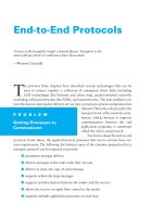
End-to-End Protocols
Victory is the beautiful, bright coloured flower. Transport is the
stem without which it could never have blossomed.
—Winston Churchill

T

he previous three chapters have described various technologies that can be
used to connect together a collection of computers: direct links (including
LAN technologies like Ethernet and token ring), packet-switched networks
(including cell-based networks like ATM), and internetworks. The next problem is to
turn this host-to-host packet delivery service into a process-to-process communication
channel. This is the role played by the
transport level of the network archiP R O B L E M
tecture, which, because it supports
communication between the end
Getting Processes to
application programs, is sometimes
Communicate
called the end-to-end protocol.
Two forces shape the end-to-end
protocol. From above, the application-level processes that use its services have certain requirements. The following list itemizes some of the common properties that a
transport protocol can be expected to provide:
■ guarantees message delivery
■ delivers messages in the same order they are sent
■ delivers at most one copy of each message
■ supports arbitrarily large messages
■ supports synchronization between the sender and the receiver
■ allows the receiver to apply flow control to the sender
■ supports multiple application processes on each host

Note that this list does not include all the functionality
that application processes might want from the network.
For example, it does not include security, which is typically
provided by protocols that sit above the transport level.
From below, the underlying network upon which the
transport protocol operates has certain limitations in the
level of service it can provide. Some of the more typical
limitations of the network are that it may
■ drop messages
■ reorder messages
■ deliver duplicate copies of a given message
■ limit messages to some finite size
■ deliver messages after an arbitrarily long delay
Such a network is said to provide a best-effort level of
service, as exemplified by the Internet.
The challenge, therefore, is to develop algorithms
that turn the less-than-desirable properties of the underlying network into the high level of service required by application programs. Different transport protocols employ
different combinations of these algorithms. This chapter
looks at these algorithms in the context of three representative services—a simple asynchronous demultiplexing
service, a reliable byte-stream service, and a request/reply
service.
In the case of the demultiplexing and byte-stream
services, we use the Internet’s UDP and TCP protocols,
respectively, to illustrate how these services are provided
in practice. In the third case, we first give a collection of
algorithms that implement the request/reply (plus other related) services and then show how these algorithms can be
combined to implement a Remote Procedure Call (RPC)
protocol. This discussion is capped off with a description
of two widely used RPC protocols—SunRPC and DCERPC—in terms of these component algorithms. Finally,

the chapter concludes with a section that discusses the
performance of the different transport protocols.

5


376

5 End-to-End Protocols

5.1 Simple Demultiplexer (UDP)
The simplest possible transport protocol is one that extends the host-to-host delivery
service of the underlying network into a process-to-process communication service.
There are likely to be many processes running on any given host, so the protocol needs
to add a level of demultiplexing, thereby allowing multiple application processes on
each host to share the network. Aside from this requirement, the transport protocol
adds no other functionality to the best-effort service provided by the underlying network. The Internet’s User Datagram Protocol (UDP) is an example of such a transport
protocol.
The only interesting issue in such a protocol is the form of the address used to
identify the target process. Although it is possible for processes to directly identify
each other with an OS-assigned process id (pid), such an approach is only practical
in a closed distributed system in which a single OS runs on all hosts and assigns each
process a unique id. A more common approach, and the one used by UDP, is for
processes to indirectly identify each other using an abstract locator, often called a port
or mailbox. The basic idea is for a source process to send a message to a port and for
the destination process to receive the message from a port.
The header for an end-to-end protocol that implements this demultiplexing function typically contains an identifier (port) for both the sender (source) and the receiver
(destination) of the message. For example, the UDP header is given in Figure 5.1. Notice
that the UDP port field is only 16 bits long. This means that there are up to 64K possible ports, clearly not enough to identify all the processes on all the hosts in the Internet.
Fortunately, ports are not interpreted across the entire Internet, but only on a single

host. That is, a process is really identified by a port on some particular host—a port,
host pair. In fact, this pair constitutes the demultiplexing key for the UDP protocol.
The next issue is how a process learns the port for the process to which it wants
to send a message. Typically, a client process initiates a message exchange with a server
0

16

31

SrcPort

DstPort

Length

Checksum
Data

Figure 5.1

Format for UDP header.


5.1 Simple Demultiplexer (UDP)

377

process. Once a client has contacted a server, the server knows the client’s port (it was
contained in the message header) and can reply to it. The real problem, therefore, is how

the client learns the server’s port in the first place. A common approach is for the server
to accept messages at a well-known port. That is, each server receives its messages at
some fixed port that is widely published, much like the emergency telephone service
available at the well-known phone number 911. In the Internet, for example, the
Domain Name Server (DNS) receives messages at well-known port 53 on each host,
the mail service listens for messages at port 25, and the Unix talk program accepts
messages at well-known port 517, and so on. This mapping is published periodically
in an RFC and is available on most Unix systems in file /etc/services. Sometimes a
well-known port is just the starting point for communication: The client and server
use the well-known port to agree on some other port that they will use for subsequent
communication, leaving the well-known port free for other clients.
An alternative strategy is to generalize this idea, so that there is only a single
well-known port—the one at which the “Port Mapper” service accepts messages. A
client would send a message to the Port Mapper’s well-known port asking for the
port it should use to talk to the “whatever” service, and the Port Mapper returns
the appropriate port. This strategy makes it easy to change the port associated with
different services over time, and for each host to use a different port for the same
service.
As just mentioned, a port is purely an abstraction. Exactly how it is implemented
differs from system to system, or more precisely, from OS to OS. For example, the
socket API described in Chapter 1 is an implementation of ports. Typically, a port is
implemented by a message queue, as illustrated in Figure 5.2. When a message arrives,
the protocol (e.g., UDP) appends the message to the end of the queue. Should the
queue be full, the message is discarded. There is no flow-control mechanism that tells
the sender to slow down. When an application process wants to receive a message,
one is removed from the front of the queue. If the queue is empty, the process blocks
until a message becomes available.
Finally, although UDP does not implement flow control or reliable/ordered delivery, it does a little more work than to simply demultiplex messages to some application
process—it also ensures the correctness of the message by the use of a checksum. (The
UDP checksum is optional in the current Internet, but it will become mandatory with

IPv6.) UDP computes its checksum over the UDP header, the contents of the message
body, and something called the pseudoheader. The pseudoheader consists of three fields
from the IP header—protocol number, source IP address, and destination IP address—
plus the UDP length field. (Yes, the UDP length field is included twice in the checksum
calculation.) UDP uses the same checksum algorithm as IP, as defined in Section 2.4.2.
The motivation behind having the pseudoheader is to verify that this message has been


378

5 End-to-End Protocols

Application
process

Application
process

Application
process

Ports

Queues

Packets
demultiplexed
UDP

Packets arrive

Figure 5.2

UDP message queue.

delivered between the correct two endpoints. For example, if the destination IP address
was modified while the packet was in transit, causing the packet to be misdelivered,
this fact would be detected by the UDP checksum.

5.2 Reliable Byte Stream (TCP)
In contrast to a simple demultiplexing protocol like UDP, a more sophisticated transport protocol is one that offers a reliable, connection-oriented, byte-stream service.
Such a service has proven useful to a wide assortment of applications because it frees
the application from having to worry about missing or reordered data. The Internet’s
Transmission Control Protocol (TCP) is probably the most widely used protocol of
this type; it is also the most carefully tuned. It is for these two reasons that this section
studies TCP in detail, although we identify and discuss alternative design choices at
the end of the section.
In terms of the properties of transport protocols given in the problem statement
at the start of this chapter, TCP guarantees the reliable, in-order delivery of a stream
of bytes. It is a full-duplex protocol, meaning that each TCP connection supports a


5.2 Reliable Byte Stream (TCP)

◮

379

pair of byte streams, one flowing in each direction. It also includes a flow-control
mechanism for each of these byte streams that allows the receiver to limit how much

data the sender can transmit at a given time. Finally, like UDP, TCP supports a demultiplexing mechanism that allows multiple application programs on any given host
to simultaneously carry on a conversation with their peers. In addition to the above
features, TCP also implements a highly tuned congestion-control mechanism. The idea
of this mechanism is to throttle how fast TCP sends data, not for the sake of keeping
the sender from overrunning the receiver, but to keep the sender from overloading
the network. A description of TCP’s congestion-control mechanism is postponed until
Chapter 6, where we discuss it in the larger context of how network resources are
fairly allocated.
Since many people confuse congestion control and flow control, we restate the
difference. Flow control involves preventing senders from overrunning the capacity of
receivers. Congestion control involves preventing too much data from being injected
into the network, thereby causing switches or links to become overloaded. Thus, flow
control is an end-to-end issue, while congestion control is concerned with how hosts
and networks interact.

5.2.1

End-to-End Issues

At the heart of TCP is the sliding window algorithm. Even though this is the same basic
algorithm we saw in Section 2.5.2, because TCP runs over the Internet rather than a
point-to-point link, there are many important differences. This subsection identifies
these differences and explains how they complicate TCP. The following subsections
then describe how TCP addresses these and other complications.
First, whereas the sliding window algorithm presented in Section 2.5.2 runs over a
single physical link that always connects the same two computers, TCP supports logical
connections between processes that are running on any two computers in the Internet.
This means that TCP needs an explicit connection establishment phase during which
the two sides of the connection agree to exchange data with each other. This difference
is analogous to having to dial up the other party, rather than having a dedicated phone

line. TCP also has an explicit connection teardown phase. One of the things that
happens during connection establishment is that the two parties establish some shared
state to enable the sliding window algorithm to begin. Connection teardown is needed
so each host knows it is OK to free this state.
Second, whereas a single physical link that always connects the same two computers has a fixed RTT, TCP connections are likely to have widely different round-trip
times. For example, a TCP connection between a host in San Francisco and a host
in Boston, which are separated by several thousand kilometers, might have an RTT


380

5 End-to-End Protocols

of 100 ms, while a TCP connection between two hosts in the same room, only a few
meters apart, might have an RTT of only 1 ms. The same TCP protocol must be able
to support both of these connections. To make matters worse, the TCP connection
between hosts in San Francisco and Boston might have an RTT of 100 ms at 3 a.m.,
but an RTT of 500 ms at 3 p.m. Variations in the RTT are even possible during a
single TCP connection that lasts only a few minutes. What this means to the sliding
window algorithm is that the timeout mechanism that triggers retransmissions must be
adaptive. (Certainly, the timeout for a point-to-point link must be a settable parameter,
but it is not necessary to adapt this timer for a particular pair of nodes.)
A third difference is that packets may be reordered as they cross the Internet,
but this is not possible on a point-to-point link where the first packet put into one
end of the link must be the first to appear at the other end. Packets that are slightly
out of order do not cause a problem since the sliding window algorithm can reorder
packets correctly using the sequence number. The real issue is how far out-of-order
packets can get, or said another way, how late a packet can arrive at the destination.
In the worst case, a packet can be delayed in the Internet until IP’s time to live (TTL)
field expires, at which time the packet is discarded (and hence there is no danger of

it arriving late). Knowing that IP throws packets away after their TTL expires, TCP
assumes that each packet has a maximum lifetime. The exact lifetime, known as the
maximum segment lifetime (MSL), is an engineering choice. The current recommended
setting is 120 seconds. Keep in mind that IP does not directly enforce this 120-second
value; it is simply a conservative estimate that TCP makes of how long a packet might
live in the Internet. The implication is significant—TCP has to be prepared for very old
packets to suddenly show up at the receiver, potentially confusing the sliding window
algorithm.
Fourth, the computers connected to a point-to-point link are generally engineered
to support the link. For example, if a link’s delay × bandwidth product is computed
to be 8 KB—meaning that a window size is selected to allow up to 8 KB of data to be
unacknowledged at a given time—then it is likely that the computers at either end of
the link have the ability to buffer up to 8 KB of data. Designing the system otherwise
would be silly. On the other hand, almost any kind of computer can be connected to the
Internet, making the amount of resources dedicated to any one TCP connection highly
variable, especially considering that any one host can potentially support hundreds of
TCP connections at the same time. This means that TCP must include a mechanism
that each side uses to “learn” what resources (e.g., how much buffer space) the other
side is able to apply to the connection. This is the flow-control issue.
Fifth, because the transmitting side of a directly connected link cannot send any
faster than the bandwidth of the link allows, and only one host is pumping data into
the link, it is not possible to unknowingly congest the link. Said another way, the load


5.2 Reliable Byte Stream (TCP)

◮

381

on the link is visible in the form of a queue of packets at the sender. In contrast, the
sending side of a TCP connection has no idea what links will be traversed to reach
the destination. For example, the sending machine might be directly connected to a
relatively fast Ethernet—and so, capable of sending data at a rate of 100 Mbps—but
somewhere out in the middle of the network, a 1.5-Mbps T1 link must be traversed.
And to make matters worse, data being generated by many different sources might be
trying to traverse this same slow link. This leads to the problem of network congestion.
Discussion of this topic is delayed until Chapter 6.
We conclude this discussion of end-to-end issues by comparing TCP’s approach to
providing a reliable/ordered delivery service with the approach used by X.25 networks.
In TCP, the underlying IP network is assumed to be unreliable and to deliver messages
out of order; TCP uses the sliding window algorithm on an end-to-end basis to provide
reliable/ordered delivery. In contrast, X.25 networks use the sliding window protocol
within the network, on a hop-by-hop basis. The assumption behind this approach is
that if messages are delivered reliably and in order between each pair of nodes along
the path between the source host and the destination host, then the end-to-end service
also guarantees reliable/ordered delivery.
The problem with this latter approach is that a sequence of hop-by-hop guarantees does not necessarily add up to an end-to-end guarantee. First, if a heterogeneous
link (say, an Ethernet) is added to one end of the path, then there is no guarantee
that this hop will preserve the same service as the other hops. Second, just because
the sliding window protocol guarantees that messages are delivered correctly from
node A to node B, and then from node B to node C, it does not guarantee that node B
behaves perfectly. For example, network nodes have been known to introduce errors
into messages while transferring them from an input buffer to an output buffer. They
have also been known to accidentally reorder messages. As a consequence of these
small windows of vulnerability, it is still necessary to provide true end-to-end checks
to guarantee reliable/ordered service, even though the lower levels of the system also
implement that functionality.
This discussion serves to illustrate one of the most important principles in system
design—the end-to-end argument. In a nutshell, the end-to-end argument says that a

function (in our example, providing reliable/ordered delivery) should not be provided
in the lower levels of the system unless it can be completely and correctly implemented
at that level. Therefore, this rule argues in favor of the TCP/IP approach. This rule is
not absolute, however. It does allow for functions to be incompletely provided at a
low level as a performance optimization. This is why it is perfectly consistent with the
end-to-end argument to perform error detection (e.g., CRC) on a hop-by-hop basis;
detecting and retransmitting a single corrupt packet across one hop is preferable to
having to retransmit an entire file end-to-end.


382

5 End-to-End Protocols

Application process

Application process

…

…

Write
bytes

Read
bytes

TCP

TCP

Send buffer

Receive buffer

Segment

Segment

…

Segment

Transmit segments

Figure 5.3

5.2.2

How TCP manages a byte stream.

Segment Format

TCP is a byte-oriented protocol, which means that the sender writes bytes into a TCP
connection and the receiver reads bytes out of the TCP connection. Although “byte
stream” describes the service TCP offers to application processes, TCP does not, itself,
transmit individual bytes over the Internet. Instead, TCP on the source host buffers
enough bytes from the sending process to fill a reasonably sized packet and then sends
this packet to its peer on the destination host. TCP on the destination host then empties

the contents of the packet into a receive buffer, and the receiving process reads from
this buffer at its leisure. This situation is illustrated in Figure 5.3, which, for simplicity,
shows data flowing in only one direction. Remember that, in general, a single TCP
connection supports byte streams flowing in both directions.
The packets exchanged between TCP peers in Figure 5.3 are called segments,
since each one carries a segment of the byte stream. Each TCP segment contains the
header schematically depicted in Figure 5.4. The relevance of most of these fields will
become apparent throughout this section. For now, we simply introduce them.
The SrcPort and DstPort fields identify the source and destination ports, respectively, just as in UDP. These two fields, plus the source and destination IP addresses,
combine to uniquely identify each TCP connection. That is, TCP’s demux key is given
by the 4-tuple
SrcPort, SrcIPAddr, DstPort, DstIPAddr

Note that because TCP connections come and go, it is possible for a connection between a particular pair of ports to be established, used to send and receive data, and
closed, and then at a later time for the same pair of ports to be involved in a second


5.2 Reliable Byte Stream (TCP)

0

10

4

383

16

31

SrcPort

DstPort
SequenceNum
Acknowledgment

0

HdrLen

Flags

AdvertisedWindow
UrgPtr

Checksum
Options (variable)
Data

Figure 5.4

TCP header format.

Data (SequenceNum)
Receiver

Sender
Acknowledgment +
AdvertisedWindow

Figure 5.5 Simplified illustration (showing only one direction) of the TCP process,
with data flow in one direction and ACKs in the other.

connection. We sometimes refer to this situation as two different incarnations of the
same connection.
The Acknowledgment, SequenceNum, and AdvertisedWindow fields are all involved in TCP’s sliding window algorithm. Because TCP is a byte-oriented protocol,
each byte of data has a sequence number; the SequenceNum field contains the sequence
number for the first byte of data carried in that segment. The Acknowledgment and
AdvertisedWindow fields carry information about the flow of data going in the other
direction. To simplify our discussion, we ignore the fact that data can flow in both
directions, and we concentrate on data that has a particular SequenceNum flowing
in one direction and Acknowledgment and AdvertisedWindow values flowing in the
opposite direction, as illustrated in Figure 5.5. The use of these three fields is described
more fully in Section 5.2.4.
The 6-bit Flags field is used to relay control information between TCP peers. The
possible flags include SYN, FIN, RESET, PUSH, URG, and ACK. The SYN and FIN flags


384

5 End-to-End Protocols

are used when establishing and terminating a TCP connection, respectively. Their use
is described in Section 5.2.3. The ACK flag is set any time the Acknowledgment field is
valid, implying that the receiver should pay attention to it. The URG flag signifies that
this segment contains urgent data. When this flag is set, the UrgPtr field indicates where
the nonurgent data contained in this segment begins. The urgent data is contained at
the front of the segment body, up to and including a value of UrgPtr bytes into the
segment. The PUSH flag signifies that the sender invoked the push operation, which

indicates to the receiving side of TCP that it should notify the receiving process of
this fact. We discuss these last two features more in Section 5.2.7. Finally, the RESET
flag signifies that the receiver has become confused—for example, because it received
a segment it did not expect to receive—and so wants to abort the connection.
Finally, the Checksum field is used in exactly the same way as for UDP—it is
computed over the TCP header, the TCP data, and the pseudoheader, which is made
up of the source address, destination address, and length fields from the IP header. The
checksum is required for TCP in both IPv4 and IPv6. Also, since the TCP header is of
variable length (options can be attached after the mandatory fields), a HdrLen field is
included that gives the length of the header in 32-bit words. This field is also known
as the Offset field, since it measures the offset from the start of the packet to the start
of the data.

5.2.3

Connection Establishment and Termination

A TCP connection begins with a client (caller) doing an active open to a server (callee).
Assuming that the server had earlier done a passive open, the two sides engage in
an exchange of messages to establish the connection. (Recall from Chapter 1 that a
party wanting to initiate a connection performs an active open, while a party willing to accept a connection does a passive open.) Only after this connection establishment phase is over do the two sides begin sending data. Likewise, as soon as
a participant is done sending data, it closes one direction of the connection, which
causes TCP to initiate a round of connection termination messages. Notice that while
connection setup is an asymmetric activity (one side does a passive open and the
other side does an active open), connection teardown is symmetric (each side has to
close the connection independently).1 Therefore, it is possible for one side to have
done a close, meaning that it can no longer send data, but for the other side to
keep the other half of the bidirectional connection open and to continue sending
data.
1

To be more precise, connection setup can be symmetric, with both sides trying to open the connection at the same
time, but the common case is for one side to do an active open and the other side to do a passive open.


5.2 Reliable Byte Stream (TCP)

Active participant
(client)

385

SYN,
Sequ
e

Passive participant
(server)

nceN

um =

x

= y,
eNum
uenc
x+1
q
e

=
S
ent
m
ACK,
g
+
d
e
N
SY
owl
Ackn
ACK,
Ackno
wledg
ment
=y+
1

Figure 5.6

Timeline for three-way handshake algorithm.

Three-Way Handshake
The algorithm used by TCP to establish and terminate a connection is called a threeway handshake. We first describe the basic algorithm and then show how it is used by
TCP. The three-way handshake involves the exchange of three messages between the
client and the server, as illustrated by the timeline given in Figure 5.6.
The idea is that two parties want to agree on a set of parameters, which, in the
case of opening a TCP connection, are the starting sequence numbers the two sides plan

to use for their respective byte streams. In general, the parameters might be any facts
that each side wants the other to know about. First, the client (the active participant)
sends a segment to the server (the passive participant) stating the initial sequence
number it plans to use (Flags = SYN, SequenceNum = x). The server then responds
with a single segment that both acknowledges the client’s sequence number (Flags =
ACK, Ack = x + 1) and states its own beginning sequence number (Flags = SYN,
SequenceNum = y). That is, both the SYN and ACK bits are set in the Flags field of this
second message. Finally, the client responds with a third segment that acknowledges
the server’s sequence number (Flags = ACK, Ack = y + 1). The reason that each
side acknowledges a sequence number that is one larger than the one sent is that
the Acknowledgment field actually identifies the “next sequence number expected,”
thereby implicitly acknowledging all earlier sequence numbers. Although not shown
in this timeline, a timer is scheduled for each of the first two segments, and if the
expected response is not received, the segment is retransmitted.
You may be asking yourself why the client and server have to exchange starting
sequence numbers with each other at connection setup time. It would be simpler if
each side simply started at some “well-known” sequence number, such as 0. In fact,


386

5 End-to-End Protocols

the TCP specification requires that each side of a connection select an initial starting
sequence number at random. The reason for this is to protect against two incarnations
of the same connection reusing the same sequence numbers too soon, that is, while
there is still a chance that a segment from an earlier incarnation of a connection might
interfere with a later incarnation of the connection.
State Transition Diagram
TCP is complex enough that its specification includes a state transition diagram. A

copy of this diagram is given in Figure 5.7. This diagram shows only the states involved in opening a connection (everything above ESTABLISHED) and in closing a
connection (everything below ESTABLISHED). Everything that goes on while a connection is open—that is, the operation of the sliding window algorithm—is hidden in
the ESTABLISHED state.

CLOSED
Active open/SYN
Passive open

Close
Close

LISTEN

SYN_RCVD

SYN/SYN + ACK
Send/SYN
SYN/SYN + ACK
ACK

ESTABLISHED

Close/FIN

FIN/ACK

Close/FIN
FIN_WAIT_1

CLOSE_WAIT

A

FIN/ACK

C

ACK
FIN_WAIT_2

K

+

Close/FIN
FI

N

/A

CLOSING

C

FIN/ACK

Figure 5.7

SYN_SENT

SYN + ACK/ACK

K

ACK Timeout after two
segment lifetimes
TIME_WAIT

TCP state transition diagram.

LAST_ACK
ACK
CLOSED


5.2 Reliable Byte Stream (TCP)

387

TCP’s state transition diagram is fairly easy to understand. Each circle denotes
a state that one end of a TCP connection can find itself in. All connections start in the
CLOSED state. As the connection progresses, the connection moves from state to state
according to the arcs. Each arc is labelled with a tag of the form event/action. Thus, if
a connection is in the LISTEN state and a SYN segment arrives (i.e., a segment with
the SYN flag set), the connection makes a transition to the SYN RCVD state and takes
the action of replying with an ACK + SYN segment.
Notice that two kinds of events trigger a state transition: (1) a segment arrives
from the peer (e.g., the event on the arc from LISTEN to SYN RCVD), or (2) the local
application process invokes an operation on TCP (e.g., the active open event on the arc
from CLOSE to SYN SENT). In other words, TCP’s state transition diagram effectively

defines the semantics of both its peer-to-peer interface and its service interface, as
defined in Section 1.3.1. The syntax of these two interfaces is given by the segment
format (as illustrated in Figure 5.4) and by some application programming interface
(an example of which is given in Section 1.4.1), respectively.
Now let’s trace the typical transitions taken through the diagram in Figure 5.7.
Keep in mind that at each end of the connection, TCP makes different transitions
from state to state. When opening a connection, the server first invokes a passive open
operation on TCP, which causes TCP to move to the LISTEN state. At some later time,
the client does an active open, which causes its end of the connection to send a SYN
segment to the server and to move to the SYN SENT state. When the SYN segment
arrives at the server, it moves to the SYN RCVD state and responds with a SYN+ACK
segment. The arrival of this segment causes the client to move to the ESTABLISHED
state and to send an ACK back to the server. When this ACK arrives, the server finally
moves to the ESTABLISHED state. In other words, we have just traced the three-way
handshake.
There are three things to notice about the connection establishment half of the
state transition diagram. First, if the client’s ACK to the server is lost, corresponding to
the third leg of the three-way handshake, then the connection still functions correctly.
This is because the client side is already in the ESTABLISHED state, so the local
application process can start sending data to the other end. Each of these data segments
will have the ACK flag set, and the correct value in the Acknowledgment field, so the
server will move to the ESTABLISHED state when the first data segment arrives.
This is actually an important point about TCP—every segment reports what sequence
number the sender is expecting to see next, even if this repeats the same sequence
number contained in one or more previous segments.
The second thing to notice about the state transition diagram is that there is a
funny transition out of the LISTEN state whenever the local process invokes a send
operation on TCP. That is, it is possible for a passive participant to identify both ends

388

5 End-to-End Protocols

of the connection (i.e., itself and the remote participant that it is willing to have connect
to it), and then to change its mind about waiting for the other side and instead actively
establish the connection. To the best of our knowledge, this is a feature of TCP that
no application process actually takes advantage of.
The final thing to notice about the diagram is the arcs that are not shown. Specifically, most of the states that involve sending a segment to the other side also schedule
a timeout that eventually causes the segment to be resent if the expected response does
not happen. These retransmissions are not depicted in the state transition diagram. If
after several tries the expected response does not arrive, TCP gives up and returns to
the CLOSED state.
Turning our attention now to the process of terminating a connection, the important thing to keep in mind is that the application process on both sides of the
connection must independently close its half of the connection. If only one side closes
the connection, then this means it has no more data to send, but it is still available
to receive data from the other side. This complicates the state transition diagram because it must account for the possibility that the two sides invoke the close operator
at the same time, as well as the possibility that first one side invokes close and then,
at some later time, the other side invokes close. Thus, on any one side there are three
combinations of transitions that get a connection from the ESTABLISHED state to the
CLOSED state:
■ This side closes first:
ESTABLISHED → FIN WAIT 1 → FIN WAIT 2 → TIME WAIT →
CLOSED.
■ The other side closes first:
ESTABLISHED → CLOSE WAIT → LAST ACK → CLOSED.
■ Both sides close at the same time:
ESTABLISHED → FIN WAIT 1 → CLOSING → TIME WAIT →
CLOSED.
There is actually a fourth, although rare, sequence of transitions that leads to the

CLOSED state; it follows the arc from FIN WAIT 1 to TIME WAIT. We leave it as an
exercise for you to figure out what combination of circumstances leads to this fourth
possibility.
The main thing to recognize about connection teardown is that a connection in
the TIME WAIT state cannot move to the CLOSED state until it has waited for two
times the maximum amount of time an IP datagram might live in the Internet (i.e.,
120 seconds). The reason for this is that while the local side of the connection has
sent an ACK in response to the other side’s FIN segment, it does not know that the
ACK was successfully delivered. As a consequence, the other side might retransmit its


5.2 Reliable Byte Stream (TCP)

389

FIN segment, and this second FIN segment might be delayed in the network. If the
connection were allowed to move directly to the CLOSED state, then another pair of
application processes might come along and open the same connection (i.e., use the
same pair of port numbers), and the delayed FIN segment from the earlier incarnation
of the connection would immediately initiate the termination of the later incarnation
of that connection.

5.2.4

Sliding Window Revisited

We are now ready to discuss TCP’s variant of the sliding window algorithm, which
serves several purposes: (1) it guarantees the reliable delivery of data, (2) it ensures
that data is delivered in order, and (3) it enforces flow control between the sender
and the receiver. TCP’s use of the sliding window algorithm is the same as we saw in

Section 2.5.2 in the case of the first two of these three functions. Where TCP differs
from the earlier algorithm is that it folds the flow-control function in as well. In
particular, rather than having a fixed-size sliding window, the receiver advertises a
window size to the sender. This is done using the AdvertisedWindow field in the TCP
header. The sender is then limited to having no more than a value of AdvertisedWindow
bytes of unacknowledged data at any given time. The receiver selects a suitable value
for AdvertisedWindow based on the amount of memory allocated to the connection
for the purpose of buffering data. The idea is to keep the sender from overrunning the
receiver’s buffer. We discuss this at greater length below.
Reliable and Ordered Delivery
To see how the sending and receiving sides of TCP interact with each other to implement reliable and ordered delivery, consider the situation illustrated in Figure 5.8.
TCP on the sending side maintains a send buffer. This buffer is used to store data

Sending application

Receiving application

TCP
LastByteWritten

LastByteAcked

LastByteSent
(a)

Figure 5.8

TCP
LastByteRead

NextByteExpected

LastByteRcvd

(b)

Relationship between TCP send buffer (a) and receive buffer (b).


390

5 End-to-End Protocols

that has been sent but not yet acknowledged, as well as data that has been written by
the sending application, but not transmitted. On the receiving side, TCP maintains a
receive buffer. This buffer holds data that arrives out of order, as well as data that is
in the correct order (i.e., there are no missing bytes earlier in the stream) but that the
application process has not yet had the chance to read.
To make the following discussion simpler to follow, we initially ignore the fact
that both the buffers and the sequence numbers are of some finite size and hence will
eventually wrap around. Also, we do not distinguish between a pointer into a buffer
where a particular byte of data is stored and the sequence number for that byte.
Looking first at the sending side, three pointers are maintained into the send buffer, each with an obvious meaning: LastByteAcked, LastByteSent, and LastByteWritten.
Clearly,
LastByteAcked ≤ LastByteSent

since the receiver cannot have acknowledged a byte that has not yet been sent, and
LastByteSent ≤ LastByteWritten

since TCP cannot send a byte that the application process has not yet written. Also

note that none of the bytes to the left of LastByteAcked need to be saved in the buffer
because they have already been acknowledged, and none of the bytes to the right of
LastByteWritten need to be buffered because they have not yet been generated.
A similar set of pointers (sequence numbers) are maintained on the receiving side:
LastByteRead, NextByteExpected, and LastByteRcvd. The inequalities are a little less intuitive, however, because of the problem of out-of-order delivery. The first relationship
LastByteRead < NextByteExpected

is true because a byte cannot be read by the application until it is received and all preceding bytes have also been received. NextByteExpected points to the byte immediately
after the latest byte to meet this criterion. Second,
NextByteExpected ≤ LastByteRcvd + 1

since, if data has arrived in order, NextByteExpected points to the byte after LastByteRcvd, whereas if data has arrived out of order, NextByteExpected points to the start of
the first gap in the data, as in Figure 5.8. Note that bytes to the left of LastByteRead
need not be buffered because they have already been read by the local application
process, and bytes to the right of LastByteRcvd need not be buffered because they have
not yet arrived.
Flow Control
Most of the above discussion is similar to that found in Section 2.5.2; the only real
difference is that this time we elaborated on the fact that the sending and receiving application processes are filling and emptying their local buffer, respectively. (The earlier


5.2 Reliable Byte Stream (TCP)

391

discussion glossed over the fact that data arriving from an upstream node was filling
the send buffer, and data being transmitted to a downstream node was emptying the
receive buffer.)
You should make sure you understand this much before proceeding because
now comes the point where the two algorithms differ more significantly. In what

follows, we reintroduce the fact that both buffers are of some finite size, denoted
MaxSendBuffer and MaxRcvBuffer, although we don’t worry about the details of how
they are implemented. In other words, we are only interested in the number of bytes
being buffered, not in where those bytes are actually stored.
Recall that in a sliding window protocol, the size of the window sets the amount
of data that can be sent without waiting for acknowledgment from the receiver. Thus,
the receiver throttles the sender by advertising a window that is no larger than the
amount of data that it can buffer. Observe that TCP on the receive side must keep
LastByteRcvd − LastByteRead ≤ MaxRcvBuffer

to avoid overflowing its buffer. It therefore advertises a window size of
AdvertisedWindow = MaxRcvBuffer − (( NextByteExpected − 1) − LastByteRead)

which represents the amount of free space remaining in its buffer. As data arrives,
the receiver acknowledges it as long as all the preceding bytes have also arrived. In
addition, LastByteRcvd moves to the right (is incremented), meaning that the advertised
window potentially shrinks. Whether or not it shrinks depends on how fast the local
application process is consuming data. If the local process is reading data just as fast as
it arrives (causing LastByteRead to be incremented at the same rate as LastByteRcvd),
then the advertised window stays open (i.e., AdvertisedWindow = MaxRcvBuffer).
If, however, the receiving process falls behind, perhaps because it performs a very
expensive operation on each byte of data that it reads, then the advertised window
grows smaller with every segment that arrives, until it eventually goes to 0.
TCP on the send side must then adhere to the advertised window it gets from
the receiver. This means that at any given time, it must ensure that
LastByteSent − LastByteAcked ≤ AdvertisedWindow

Said another way, the sender computes an effective window that limits how much data
it can send:
EffectiveWindow = AdvertisedWindow − ( LastByteSent − LastByteAcked)

Clearly, EffectiveWindow must be greater than 0 before the source can send more data.
It is possible, therefore, that a segment arrives acknowledging x bytes, thereby allowing
the sender to increment LastByteAcked by x, but because the receiving process was not
reading any data, the advertised window is now x bytes smaller than the time before.


392

5 End-to-End Protocols

In such a situation, the sender would be able to free buffer space, but not to send any
more data.
All the while this is going on, the send side must also make sure that the local
application process does not overflow the send buffer, that is, that
LastByteWritten − LastByteAcked ≤ MaxSendBuffer

If the sending process tries to write y bytes to TCP, but
( LastByteWritten − LastByteAcked) + y > MaxSendBuffer

◮

then TCP blocks the sending process and does not allow it to generate more data.
It is now possible to understand how a slow receiving process ultimately stops
a fast sending process. First, the receive buffer fills up, which means the advertised
window shrinks to 0. An advertised window of 0 means that the sending side cannot
transmit any data, even though data it has previously sent has been successfully acknowledged. Finally, not being able to transmit any data means that the send buffer
fills up, which ultimately causes TCP to block the sending process. As soon as the
receiving process starts to read data again, the receive-side TCP is able to open its window back up, which allows the send-side TCP to transmit data out of its buffer. When
this data is eventually acknowledged, LastByteAcked is incremented, the buffer space

holding this acknowledged data becomes free, and the sending process is unblocked
and allowed to proceed.
There is only one remaining detail that must be resolved—how does the sending
side know that the advertised window is no longer 0? As mentioned above, TCP always
sends a segment in response to a received data segment, and this response contains the
latest values for the Acknowledge and AdvertisedWindow fields, even if these values
have not changed since the last time they were sent. The problem is this. Once the
receive side has advertised a window size of 0, the sender is not permitted to send
any more data, which means it has no way to discover that the advertised window
is no longer 0 at some time in the future. TCP on the receive side does not spontaneously send nondata segments; it only sends them in response to an arriving data
segment.
TCP deals with this situation as follows. Whenever the other side advertises a
window size of 0, the sending side persists in sending a segment with 1 byte of data
every so often. It knows that this data will probably not be accepted, but it tries
anyway, because each of these 1-byte segments triggers a response that contains the
current advertised window. Eventually, one of these 1-byte probes triggers a response
that reports a nonzero advertised window.
Note that the reason the sending side periodically sends this probe segment is
that TCP is designed to make the receive side as simple as possible—it simply responds


5.2 Reliable Byte Stream (TCP)

393

to segments from the sender, and it never initiates any activity on its own. This is
an example of a well-recognized (although not universally applied) protocol design
rule, which, for lack of a better name, we call the smart sender/dumb receiver rule.
Recall that we saw another example of this rule when we discussed the use of NAKs
in Section 2.5.2.

Protecting against Wraparound
This subsection and the next consider the size of the SequenceNum and AdvertisedWindow fields and the implications of their sizes on TCP’s correctness and performance.
TCP’s SequenceNum field is 32 bits long, and its AdvertisedWindow field is 16 bits
long, meaning that TCP has easily satisfied the requirement of the sliding window algorithm that the sequence number space be twice as big as the window size: 232 ≫ 2×216 .
However, this requirement is not the interesting thing about these two fields. Consider
each field in turn.
The relevance of the 32-bit sequence number space is that the sequence number
used on a given connection might wrap around—a byte with sequence number x could
be sent at one time, and then at a later time a second byte with the same sequence
number x might be sent. Once again, we assume that packets cannot survive in the
Internet for longer than the recommended MSL. Thus, we currently need to make
sure that the sequence number does not wrap around within a 120-second period of
time. Whether or not this happens depends on how fast data can be transmitted over
the Internet, that is, how fast the 32-bit sequence number space can be consumed.
(This discussion assumes that we are trying to consume the sequence number space as
fast as possible, but of course we will be if we are doing our job of keeping the pipe
full.) Table 5.1 shows how long it takes for the sequence number to wrap around on
networks with various bandwidths.
As you can see, the 32-bit sequence number space is adequate for today’s networks, but given that OC-48 links currently exist in the Internet backbone, it won’t
be long until individual TCP connections want to run at 622-Mbps speeds or higher.
Fortunately, the IETF has already worked out an extension to TCP that effectively
extends the sequence number space to protect against the sequence number wrapping
around. This and related extensions are described in Section 5.2.8.
Keeping the Pipe Full
The relevance of the 16-bit AdvertisedWindow field is that it must be big enough
to allow the sender to keep the pipe full. Clearly, the receiver is free not to open
the window as large as the AdvertisedWindow field allows; we are interested in the
situation in which the receiver has enough buffer space to handle as much data as the
largest possible AdvertisedWindow allows.

394

5 End-to-End Protocols

Bandwidth

Time until Wraparound

T1 (1.5 Mbps)

6.4 hours

Ethernet (10 Mbps)

57 minutes

T3 (45 Mbps)

13 minutes

FDDI (100 Mbps)

6 minutes

STS-3 (155 Mbps)

4 minutes

STS-12 (622 Mbps)

55 seconds

STS-24 (1.2 Gbps)

28 seconds

Table 5.1

Time until 32-bit sequence number space wraps around.

Bandwidth

Delay × Bandwidth Product

T1 (1.5 Mbps)

18 KB

Ethernet (10 Mbps)

122 KB

T3 (45 Mbps)

549 KB

FDDI (100 Mbps)

1.2 MB

STS-3 (155 Mbps)

1.8 MB

STS-12 (622 Mbps)

7.4 MB

STS-24 (1.2 Gbps)

14.8 MB

Table 5.2

Required window size for 100-ms RTT.

In this case, it is not just the network bandwidth but the delay × bandwidth
product that dictates how big the AdvertisedWindow field needs to be—the window
needs to be opened far enough to allow a full delay × bandwidth product’s worth of
data to be transmitted. Assuming an RTT of 100 ms (a typical number for a crosscountry connection in the U.S.), Table 5.2 gives the delay × bandwidth product for
several network technologies.
As you can see, TCP’s AdvertisedWindow field is in even worse shape than its
SequenceNum field—it is not big enough to handle even a T3 connection across the
continental United States, since a 16-bit field allows us to advertise a window of only
64 KB. The very same TCP extension mentioned above (see Section 5.2.8) provides a
mechanism for effectively increasing the size of the advertised window.


5.2 Reliable Byte Stream (TCP)

5.2.5

395

Triggering Transmission

We next consider a surprisingly subtle issue: how TCP decides to transmit a segment. As
described earlier, TCP supports a byte-stream abstraction, that is, application programs
write bytes into the stream, and it is up to TCP to decide that it has enough bytes to
send a segment. What factors govern this decision?
If we ignore the possibility of flow control—that is, we assume the window is
wide open, as would be the case when a connection first starts—then TCP has three
mechanisms to trigger the transmission of a segment. First, TCP maintains a variable,
typically called the maximum segment size (MSS), and it sends a segment as soon as it
has collected MSS bytes from the sending process. MSS is usually set to the size of the
largest segment TCP can send without causing the local IP to fragment. That is, MSS
is set to the MTU of the directly connected network, minus the size of the TCP and IP
headers. The second thing that triggers TCP to transmit a segment is that the sending
process has explicitly asked it to do so. Specifically, TCP supports a push operation,
and the sending process invokes this operation to effectively flush the buffer of unsent
bytes. The final trigger for transmitting a segment is that a timer fires; the resulting
segment contains as many bytes as are currently buffered for transmission. However,
as we will soon see, this “timer” isn’t exactly what you expect.

Silly Window Syndrome
Of course, we can’t just ignore flow control, which plays an obvious role in throttling
the sender. If the sender has MSS bytes of data to send and the window is open at least
that much, then the sender transmits a full segment. Suppose, however, that the sender
is accumulating bytes to send, but the window is currently closed. Now suppose an

ACK arrives that effectively opens the window enough for the sender to transmit, say,
MSS/2 bytes. Should the sender transmit a half-full segment or wait for the window
to open to a full MSS? The original specification was silent on this point, and early
implementations of TCP decided to go ahead and transmit a half-full segment. After
all, there is no telling how long it will be before the window opens further.
It turns out that the strategy of aggressively taking advantage of any available
window leads to a situation now known as the silly window syndrome. Figure 5.9
helps visualize what happens. If you think of a TCP stream as a conveyer belt with
“full” containers (data segments) going in one direction and empty containers (ACKs)
going in the reverse direction, then MSS-sized segments correspond to large containers
and 1-byte segments correspond to very small containers. If the sender aggressively fills
an empty container as soon as it arrives, then any small container introduced into the
system remains in the system indefinitely. That is, it is immediately filled and emptied
at each end, and never coalesced with adjacent containers to create larger containers.


396

5 End-to-End Protocols

Receiver

Sender

Figure 5.9

Silly window syndrome.

This scenario was discovered when early implementations of TCP regularly found
themselves filling the network with tiny segments.

Note that the silly window syndrome is only a problem when either the sender
transmits a small segment or the receiver opens the window a small amount. If neither
of these happens, then the small container is never introduced into the stream. It’s
not possible to outlaw sending small segments; for example, the application might
do a push after sending a single byte. It is possible, however, to keep the receiver
from introducing a small container (i.e., a small open window). The rule is that after
advertizing a zero window, the receiver must wait for space equal to an MSS before it
advertises an open window.
Since we can’t eliminate the possibility of a small container being introduced into
the stream, we also need mechanisms to coalesce them. The receiver can do this by
delaying ACKs—sending one combined ACK rather than multiple smaller ones—but
this is only a partial solution because the receiver has no way of knowing how long it is
safe to delay waiting either for another segment to arrive or for the application to read
more data (thus opening the window). The ultimate solution falls to the sender, which
brings us back to our original issue: When does the TCP sender decide to transmit a
segment?

Nagle’s Algorithm
Returning to the TCP sender, if there is data to send but the window is open less than
MSS, then we may want to wait some amount of time before sending the available
data, but the question is, how long? If we wait too long, then we hurt interactive
applications like Telnet. If we don’t wait long enough, then we risk sending a bunch
of tiny packets and falling into the silly window syndrome. The answer is to introduce
a timer and to transmit when the timer expires.
While we could use a clock-based timer—for example, one that fires every 100
ms—Nagle introduced an elegant self-clocking solution. The idea is that as long as TCP
has any data in flight, the sender will eventually receive an ACK. This ACK can be


5.2 Reliable Byte Stream (TCP)

397

treated like a timer firing, triggering the transmission of more data. Nagle’s algorithm
provides a simple, unified rule for deciding when to transmit:
When the application produces data to send
if both the available data and the window ≥ MSS
send a full segment
else

if there is unACKed data in flight
buffer the new data until an ACK arrives
else
send all the new data now

In other words, it’s always OK to send a full segment if the window allows.
It’s also OK to immediately send a small amount of data if there are currently no
segments in transit, but if there is anything in flight, the sender must wait for an ACK
before transmiting the next segment. Thus, an interactive application like Telnet that
continually writes one byte at a time will send data at a rate of one segment per RTT.
Some segments will contain a single byte, while others will contain as many bytes as
the user was able to type in one round-trip time. Because some applications cannot
afford such a delay for each write they do to a TCP connection, the socket interface
allows applications to turn off Nagle’s algorithm by setting the TCP NODELAY option.
Setting this option means that data is transmitted as soon as possible.

5.2.6

Adaptive Retransmission

Because TCP guarantees the reliable delivery of data, it retransmits each segment if an
ACK is not received in a certain period of time. TCP sets this timeout as a function of
the RTT it expects between the two ends of the connection. Unfortunately, given the
range of possible RTTs between any pair of hosts in the Internet, as well as the variation in RTT between the same two hosts over time, choosing an appropriate timeout
value is not that easy. To address this problem, TCP uses an adaptive retransmission
mechanism. We now describe this mechanism and how it has evolved over time as the
Internet community has gained more experience using TCP.
Original Algorithm
We begin with a simple algorithm for computing a timeout value between a pair of
hosts. This is the algorithm that was originally described in the TCP specification—
and the following description presents it in those terms—but it could be used by any
end-to-end protocol.
The idea is to keep a running average of the RTT and then to compute the timeout
as a function of this RTT. Specifically, every time TCP sends a data segment, it records


398

5 End-to-End Protocols

the time. When an ACK for that segment arrives, TCP reads the time again and then
takes the difference between these two times as a SampleRTT. TCP then computes
an EstimatedRTT as a weighted average between the previous estimate and this new
sample. That is,
EstimatedRTT = α × EstimatedRTT + ( 1 − α) × SampleRTT

The parameter α is selected to smooth the EstimatedRTT. A small α tracks changes in
the RTT but is perhaps too heavily influenced by temporary fluctuations. On the other
hand, a large α is more stable but perhaps not quick enough to adapt to real changes.
The original TCP specification recommended a setting of α between 0.8 and 0.9. TCP

then uses EstimatedRTT to compute the timeout in a rather conservative way:
TimeOut = 2 × EstimatedRTT

Karn/Partridge Algorithm
After several years of use on the Internet, a rather obvious flaw was discovered in
this simple algorithm. The problem was that an ACK does not really acknowledge a
transmission; it actually acknowledges the receipt of data. In other words, whenever
a segment is retransmitted and then an ACK arrives at the sender, it is impossible to
determine if this ACK should be associated with the first or the second transmission
of the segment for the purpose of measuring the sample RTT. It is necessary to know
which transmission to associate it with so as to compute an accurate SampleRTT. As
illustrated in Figure 5.10, if you assume that the ACK is for the original transmission
but it was really for the second, then the SampleRTT is too large (a), while if you
assume that the ACK is for the second transmission but it was actually for the first,
then the SampleRTT is too small (b).
Sender

Orig

tran

Retr

inal

smis

ansm

Receiver

sion

SampleRTT

inal

SampleRTT

Sender

Receiver

Orig

issio

n

ACK

smis

sion

ACK
Retr
an

smis

(a)

Figure 5.10 Associating
(b) retransmission.

tran

sion

(b)

the

ACK

with

(a)

original

transmission

versus