Ebook Introduction to algorithms (3rd edition) Part 2

21

Data Structures for Disjoint Sets

Some applications involve grouping n distinct elements into a collection of disjoint
sets. These applications often need to perform two operations in particular: finding
the unique set that contains a given element and uniting two sets. This chapter
explores methods for maintaining a data structure that supports these operations.
Section 21.1 describes the operations supported by a disjoint-set data structure
and presents a simple application. In Section 21.2, we look at a simple linked-list
implementation for disjoint sets. Section 21.3 presents a more efficient representation using rooted trees. The running time using the tree representation is theoretically superlinear, but for all practical purposes it is linear. Section 21.4 defines
and discusses a very quickly growing function and its very slowly growing inverse,
which appears in the running time of operations on the tree-based implementation,
and then, by a complex amortized analysis, proves an upper bound on the running
time that is just barely superlinear.

21.1 Disjoint-set operations
A disjoint-set data structure maintains a collection S D fS1 ; S2 ; : : : ; Sk g of disjoint dynamic sets. We identify each set by a representative, which is some member of the set. In some applications, it doesn’t matter which member is used as the
representative; we care only that if we ask for the representative of a dynamic set
twice without modifying the set between the requests, we get the same answer both
times. Other applications may require a prespecified rule for choosing the representative, such as choosing the smallest member in the set (assuming, of course,
that the elements can be ordered).
As in the other dynamic-set implementations we have studied, we represent each
element of a set by an object. Letting x denote an object, we wish to support the
following operations:


562

Chapter 21 Data Structures for Disjoint Sets

M AKE -S ET .x/ creates a new set whose only member (and thus representative)
is x. Since the sets are disjoint, we require that x not already be in some other
set.
U NION .x; y/ unites the dynamic sets that contain x and y, say Sx and Sy , into a
new set that is the union of these two sets. We assume that the two sets are disjoint prior to the operation. The representative of the resulting set is any member
of Sx [ Sy , although many implementations of U NION specifically choose the
representative of either Sx or Sy as the new representative. Since we require
the sets in the collection to be disjoint, conceptually we destroy sets Sx and Sy ,
removing them from the collection S . In practice, we often absorb the elements
of one of the sets into the other set.
F IND -S ET .x/ returns a pointer to the representative of the (unique) set containing x.
Throughout this chapter, we shall analyze the running times of disjoint-set data
structures in terms of two parameters: n, the number of M AKE -S ET operations,
and m, the total number of M AKE -S ET, U NION, and F IND -S ET operations. Since
the sets are disjoint, each U NION operation reduces the number of sets by one.
After n 1 U NION operations, therefore, only one set remains. The number of
U NION operations is thus at most n 1. Note also that since the M AKE -S ET
operations are included in the total number of operations m, we have m n. We
assume that the n M AKE -S ET operations are the first n operations performed.
An application of disjoint-set data structures
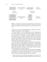
One of the many applications of disjoint-set data structures arises in determining the connected components of an undirected graph (see Section B.4). Figure 21.1(a), for example, shows a graph with four connected components.
The procedure C ONNECTED -C OMPONENTS that follows uses the disjoint-set
operations to compute the connected components of a graph. Once C ONNECTED C OMPONENTS has preprocessed the graph, the procedure S AME -C OMPONENT
answers queries about whether two vertices are in the same connected component.1
(In pseudocode, we denote the set of vertices of a graph G by G:V and the set of
edges by G:E.)

1 When the edges of the graph are static—not changing over time—we can compute the connected
components faster by using depth-first search (Exercise 22.3-12). Sometimes, however, the edges
are added dynamically and we need to maintain the connected components as each edge is added. In

this case, the implementation given here can be more efficient than running a new depth-first search
for each new edge.


21.1 Disjoint-set operations

a

b

e

c

d

g

563

f

h

j

i
(a)

Edge processed

initial sets
(b,d)
(e,g)
(a,c)
(h,i)
(a,b)
(e, f )
(b,c)

{a}
{a}
{a}
{a,c}
{a,c}
{a,b,c,d}
{a,b,c,d}
{a,b,c,d}

Collection of disjoint sets
{b}
{c} {d} {e}
{f} {g}
{b,d} {c}
{e}
{f} {g}
{b,d} {c}
{e,g}
{f}
{b,d}
{e,g}

{f}
{b,d}
{e,g}
{f}
{e,g}
{f}
{e, f,g}
{e, f,g}

{h}
{h}
{h}
{h}
{h,i}
{h,i}
{h,i}
{h,i}

{i}
{i}
{i}
{i}

{j}
{j}
{j}
{j}
{j}
{j}
{j}

{j}

(b)

Figure 21.1 (a) A graph with four connected components: fa; b; c; d g, fe; f; gg, fh; ig, and fj g.
(b) The collection of disjoint sets after processing each edge.

C ONNECTED -C OMPONENTS .G/
1 for each vertex 2 G:V
2
M AKE -S ET . /
3 for each edge .u; / 2 G:E
4
if F IND -S ET .u/ ¤ F IND -S ET . /
5
U NION .u; /
S AME -C OMPONENT .u; /
1 if F IND -S ET .u/ == F IND -S ET . /
2
return TRUE
3 else return FALSE
The procedure C ONNECTED -C OMPONENTS initially places each vertex in its
own set. Then, for each edge .u; /, it unites the sets containing u and . By
Exercise 21.1-2, after processing all the edges, two vertices are in the same connected component if and only if the corresponding objects are in the same set.
Thus, C ONNECTED -C OMPONENTS computes sets in such a way that the procedure S AME -C OMPONENT can determine whether two vertices are in the same con-


564

Chapter 21 Data Structures for Disjoint Sets

nected component. Figure 21.1(b) illustrates how C ONNECTED -C OMPONENTS
computes the disjoint sets.
In an actual implementation of this connected-components algorithm, the representations of the graph and the disjoint-set data structure would need to reference
each other. That is, an object representing a vertex would contain a pointer to
the corresponding disjoint-set object, and vice versa. These programming details
depend on the implementation language, and we do not address them further here.
Exercises
21.1-1
Suppose that C ONNECTED -C OMPONENTS is run on the undirected graph G D
.V; E/, where V D fa; b; c; d; e; f; g; h; i; j; kg and the edges of E are processed in the order .d; i/; .f; k/; .g; i/; .b; g/; .a; h/; .i; j /; .d; k/; .b; j /; .d; f /;
.g; j /; .a; e/. List the vertices in each connected component after each iteration of
lines 3–5.
21.1-2
Show that after all edges are processed by C ONNECTED -C OMPONENTS, two vertices are in the same connected component if and only if they are in the same set.
21.1-3
During the execution of C ONNECTED -C OMPONENTS on an undirected graph G D
.V; E/ with k connected components, how many times is F IND -S ET called? How
many times is U NION called? Express your answers in terms of jV j, jEj, and k.

21.2 Linked-list representation of disjoint sets
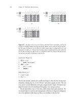
Figure 21.2(a) shows a simple way to implement a disjoint-set data structure: each
set is represented by its own linked list. The object for each set has attributes head,
pointing to the first object in the list, and tail, pointing to the last object. Each
object in the list contains a set member, a pointer to the next object in the list, and
a pointer back to the set object. Within each linked list, the objects may appear in
any order. The representative is the set member in the first object in the list.
With this linked-list representation, both M AKE -S ET and F IND -S ET are easy,
requiring O.1/ time. To carry out M AKE -S ET .x/, we create a new linked list
whose only object is x. For F IND -S ET .x/, we just follow the pointer from x back

to its set object and then return the member in the object that head points to. For
example, in Figure 21.2(a), the call F IND -S ET .g/ would return f .


21.2 Linked-list representation of disjoint sets

(a)

f

g

565

d

c

head

h

e

b

head

S1

S2
tail

tail

f

(b)

g

d

c

h

e

b

head
S1
tail

Figure 21.2 (a) Linked-list representations of two sets. Set S1 contains members d , f , and g, with
representative f , and set S2 contains members b, c, e, and h, with representative c. Each object in
the list contains a set member, a pointer to the next object in the list, and a pointer back to the set
object. Each set object has pointers head and tail to the first and last objects, respectively. (b) The
result of U NION.g; e/, which appends the linked list containing e to the linked list containing g. The

representative of the resulting set is f . The set object for e’s list, S2 , is destroyed.

A simple implementation of union
The simplest implementation of the U NION operation using the linked-list set representation takes significantly more time than M AKE -S ET or F IND -S ET. As Figure 21.2(b) shows, we perform U NION .x; y/ by appending y’s list onto the end
of x’s list. The representative of x’s list becomes the representative of the resulting
set. We use the tail pointer for x’s list to quickly find where to append y’s list. Because all members of y’s list join x’s list, we can destroy the set object for y’s list.
Unfortunately, we must update the pointer to the set object for each object originally on y’s list, which takes time linear in the length of y’s list. In Figure 21.2, for
example, the operation U NION .g; e/ causes pointers to be updated in the objects
for b, c, e, and h.
In fact, we can easily construct a sequence of m operations on n objects that
requires ‚.n2 / time. Suppose that we have objects x1 ; x2 ; : : : ; xn . We execute
the sequence of n M AKE -S ET operations followed by n 1 U NION operations
shown in Figure 21.3, so that m D 2n 1. We spend ‚.n/ time performing the n
M AKE -S ET operations. Because the ith U NION operation updates i objects, the
total number of objects updated by all n 1 U NION operations is


566

Chapter 21 Data Structures for Disjoint Sets

Operation
M AKE -S ET.x1 /
M AKE -S ET.x2 /
::
:
M AKE -S ET.xn /
U NION.x2 ; x1 /
U NION.x3 ; x2 /
U NION.x4 ; x3 /

::
:
U NION.xn ; xn 1 /

Number of objects updated
1
1
::
:
1
1
2
3
::
:
n 1

Figure 21.3 A sequence of 2n 1 operations on n objects that takes ‚.n2 / time, or ‚.n/ time
per operation on average, using the linked-list set representation and the simple implementation of
U NION.
n 1
X

i D ‚.n2 / :

i D1

The total number of operations is 2n 1, and so each operation on average requires
‚.n/ time. That is, the amortized time of an operation is ‚.n/.
A weighted-union heuristic

In the worst case, the above implementation of the U NION procedure requires an
average of ‚.n/ time per call because we may be appending a longer list onto
a shorter list; we must update the pointer to the set object for each member of
the longer list. Suppose instead that each list also includes the length of the list
(which we can easily maintain) and that we always append the shorter list onto the
longer, breaking ties arbitrarily. With this simple weighted-union heuristic, a single U NION operation can still take .n/ time if both sets have .n/ members. As
the following theorem shows, however, a sequence of m M AKE -S ET, U NION, and
F IND -S ET operations, n of which are M AKE -S ET operations, takes O.m C n lg n/
time.
Theorem 21.1
Using the linked-list representation of disjoint sets and the weighted-union heuristic, a sequence of m M AKE -S ET, U NION, and F IND -S ET operations, n of which
are M AKE -S ET operations, takes O.m C n lg n/ time.


21.2 Linked-list representation of disjoint sets

567

Proof Because each U NION operation unites two disjoint sets, we perform at
most n 1 U NION operations over all. We now bound the total time taken by these
U NION operations. We start by determining, for each object, an upper bound on the
number of times the object’s pointer back to its set object is updated. Consider a
particular object x. We know that each time x’s pointer was updated, x must have
started in the smaller set. The first time x’s pointer was updated, therefore, the
resulting set must have had at least 2 members. Similarly, the next time x’s pointer
was updated, the resulting set must have had at least 4 members. Continuing on,
we observe that for any k Ä n, after x’s pointer has been updated dlg ke times,
the resulting set must have at least k members. Since the largest set has at most n
members, each object’s pointer is updated at most dlg ne times over all the U NION
operations. Thus the total time spent updating object pointers over all U NION

operations is O.n lg n/. We must also account for updating the tail pointers and
the list lengths, which take only ‚.1/ time per U NION operation. The total time
spent in all U NION operations is thus O.n lg n/.
The time for the entire sequence of m operations follows easily. Each M AKE S ET and F IND -S ET operation takes O.1/ time, and there are O.m/ of them. The
total time for the entire sequence is thus O.m C n lg n/.
Exercises
21.2-1
Write pseudocode for M AKE -S ET, F IND -S ET, and U NION using the linked-list
representation and the weighted-union heuristic. Make sure to specify the attributes
that you assume for set objects and list objects.
21.2-2
Show the data structure that results and the answers returned by the F IND -S ET
operations in the following program. Use the linked-list representation with the
weighted-union heuristic.
1
2
3
4
5
6
7
8
9
10
11

for i D 1 to 16
M AKE -S ET .xi /
for i D 1 to 15 by 2
U NION .xi ; xi C1 /

for i D 1 to 13 by 4
U NION .xi ; xi C2 /
U NION.x1 ; x5 /
U NION.x11 ; x13 /
U NION.x1 ; x10 /
F IND -S ET .x2 /
F IND -S ET .x9 /


568

Chapter 21 Data Structures for Disjoint Sets

Assume that if the sets containing xi and xj have the same size, then the operation
U NION .xi ; xj / appends xj ’s list onto xi ’s list.
21.2-3
Adapt the aggregate proof of Theorem 21.1 to obtain amortized time bounds
of O.1/ for M AKE -S ET and F IND -S ET and O.lg n/ for U NION using the linkedlist representation and the weighted-union heuristic.
21.2-4
Give a tight asymptotic bound on the running time of the sequence of operations in
Figure 21.3 assuming the linked-list representation and the weighted-union heuristic.
21.2-5
Professor Gompers suspects that it might be possible to keep just one pointer in
each set object, rather than two (head and tail), while keeping the number of pointers in each list element at two. Show that the professor’s suspicion is well founded
by describing how to represent each set by a linked list such that each operation
has the same running time as the operations described in this section. Describe
also how the operations work. Your scheme should allow for the weighted-union
heuristic, with the same effect as described in this section. (Hint: Use the tail of a
linked list as its set’s representative.)
21.2-6

Suggest a simple change to the U NION procedure for the linked-list representation
that removes the need to keep the tail pointer to the last object in each list. Whether
or not the weighted-union heuristic is used, your change should not change the
asymptotic running time of the U NION procedure. (Hint: Rather than appending
one list to another, splice them together.)

21.3 Disjoint-set forests
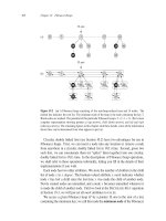
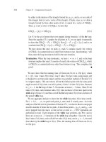
In a faster implementation of disjoint sets, we represent sets by rooted trees, with
each node containing one member and each tree representing one set. In a disjointset forest, illustrated in Figure 21.4(a), each member points only to its parent. The
root of each tree contains the representative and is its own parent. As we shall
see, although the straightforward algorithms that use this representation are no
faster than ones that use the linked-list representation, by introducing two heuristics—“union by rank” and “path compression”—we can achieve an asymptotically
optimal disjoint-set data structure.


21.3 Disjoint-set forests

c
h

569

f
e

f

d

b

g

(a)

c
h
b

d
e

g

(b)

Figure 21.4 A disjoint-set forest. (a) Two trees representing the two sets of Figure 21.2. The
tree on the left represents the set fb; c; e; hg, with c as the representative, and the tree on the right
represents the set fd; f; gg, with f as the representative. (b) The result of U NION.e; g/.

We perform the three disjoint-set operations as follows. A M AKE -S ET operation
simply creates a tree with just one node. We perform a F IND -S ET operation by
following parent pointers until we find the root of the tree. The nodes visited on
this simple path toward the root constitute the find path. A U NION operation,
shown in Figure 21.4(b), causes the root of one tree to point to the root of the other.
Heuristics to improve the running time
So far, we have not improved on the linked-list implementation. A sequence of
n 1 U NION operations may create a tree that is just a linear chain of n nodes. By
using two heuristics, however, we can achieve a running time that is almost linear
in the total number of operations m.

The first heuristic, union by rank, is similar to the weighted-union heuristic we
used with the linked-list representation. The obvious approach would be to make
the root of the tree with fewer nodes point to the root of the tree with more nodes.
Rather than explicitly keeping track of the size of the subtree rooted at each node,
we shall use an approach that eases the analysis. For each node, we maintain a
rank, which is an upper bound on the height of the node. In union by rank, we
make the root with smaller rank point to the root with larger rank during a U NION
operation.
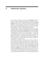
The second heuristic, path compression, is also quite simple and highly effective. As shown in Figure 21.5, we use it during F IND -S ET operations to make each
node on the find path point directly to the root. Path compression does not change
any ranks.


570

Chapter 21 Data Structures for Disjoint Sets

f

e
f
d

c

a

b

c

d

e

b

a

(a)

(b)

Figure 21.5 Path compression during the operation F IND -S ET . Arrows and self-loops at roots are
omitted. (a) A tree representing a set prior to executing F IND -S ET.a/. Triangles represent subtrees
whose roots are the nodes shown. Each node has a pointer to its parent. (b) The same set after
executing F IND -S ET.a/. Each node on the find path now points directly to the root.

Pseudocode for disjoint-set forests
To implement a disjoint-set forest with the union-by-rank heuristic, we must keep
track of ranks. With each node x, we maintain the integer value x:rank, which is
an upper bound on the height of x (the number of edges in the longest simple path
between x and a descendant leaf). When M AKE -S ET creates a singleton set, the
single node in the corresponding tree has an initial rank of 0. Each F IND -S ET operation leaves all ranks unchanged. The U NION operation has two cases, depending
on whether the roots of the trees have equal rank. If the roots have unequal rank,
we make the root with higher rank the parent of the root with lower rank, but the
ranks themselves remain unchanged. If, instead, the roots have equal ranks, we
arbitrarily choose one of the roots as the parent and increment its rank.
Let us put this method into pseudocode. We designate the parent of node x
by x:p. The L INK procedure, a subroutine called by U NION, takes pointers to two

roots as inputs.


21.3 Disjoint-set forests

571

M AKE -S ET .x/
1 x:p D x
2 x:rank D 0
U NION .x; y/
1 L INK .F IND -S ET .x/; F IND -S ET .y//
L INK .x; y/
1 if x:rank > y:rank
2
y:p D x
3 else x:p D y
4
if x:rank == y:rank
5
y:rank D y:rank C 1
The F IND -S ET procedure with path compression is quite simple:
F IND -S ET .x/
1 if x ¤ x:p
2
x:p D F IND -S ET .x:p/
3 return x:p
The F IND -S ET procedure is a two-pass method: as it recurses, it makes one pass
up the find path to find the root, and as the recursion unwinds, it makes a second
pass back down the find path to update each node to point directly to the root. Each

call of F IND -S ET .x/ returns x:p in line 3. If x is the root, then F IND -S ET skips
line 2 and instead returns x:p, which is x; this is the case in which the recursion
bottoms out. Otherwise, line 2 executes, and the recursive call with parameter x:p
returns a pointer to the root. Line 2 updates node x to point directly to the root,
and line 3 returns this pointer.
Effect of the heuristics on the running time
Separately, either union by rank or path compression improves the running time of
the operations on disjoint-set forests, and the improvement is even greater when
we use the two heuristics together. Alone, union by rank yields a running time
of O.m lg n/ (see Exercise 21.4-4), and this bound is tight (see Exercise 21.3-3).
Although we shall not prove it here, for a sequence of n M AKE -S ET operations (and hence at most n 1 U NION operations) and f F IND -S ET operations, the path-compression heuristic alone gives a worst-case running time of
‚.n C f .1 C log2Cf =n n//.


572

Chapter 21 Data Structures for Disjoint Sets

When we use both union by rank and path compression, the worst-case running
time is O.m ˛.n//, where ˛.n/ is a very slowly growing function, which we define in Section 21.4. In any conceivable application of a disjoint-set data structure,
˛.n/ Ä 4; thus, we can view the running time as linear in m in all practical situations. Strictly speaking, however, it is superlinear. In Section 21.4, we prove this
upper bound.
Exercises
21.3-1
Redo Exercise 21.2-2 using a disjoint-set forest with union by rank and path compression.
21.3-2
Write a nonrecursive version of F IND -S ET with path compression.
21.3-3
Give a sequence of m M AKE -S ET, U NION, and F IND -S ET operations, n of which
are M AKE -S ET operations, that takes .m lg n/ time when we use union by rank

only.
21.3-4
Suppose that we wish to add the operation P RINT-S ET .x/, which is given a node x
and prints all the members of x’s set, in any order. Show how we can add just
a single attribute to each node in a disjoint-set forest so that P RINT-S ET .x/ takes
time linear in the number of members of x’s set and the asymptotic running times
of the other operations are unchanged. Assume that we can print each member of
the set in O.1/ time.
21.3-5 ?
Show that any sequence of m M AKE -S ET, F IND -S ET, and L INK operations, where
all the L INK operations appear before any of the F IND -S ET operations, takes only
O.m/ time if we use both path compression and union by rank. What happens in
the same situation if we use only the path-compression heuristic?


21.4 Analysis of union by rank with path compression

573

? 21.4 Analysis of union by rank with path compression
As noted in Section 21.3, the combined union-by-rank and path-compression heuristic runs in time O.m ˛.n// for m disjoint-set operations on n elements. In this
section, we shall examine the function ˛ to see just how slowly it grows. Then we
prove this running time using the potential method of amortized analysis.
A very quickly growing function and its very slowly growing inverse
For integers k 0 and j 1, we define the function Ak .j / as
(
j C1
if k D 0 ;
Ak .j / D
.j C1/

Ak 1 .j / if k 1 ;
C1/
where the expression A.j
k 1 .j / uses the functional-iteration notation given in Sec.0/
1.
tion 3.2. Specifically, Ak 1 .j / D j and A.ik / 1 .j / D Ak 1 .Ak.i 11/ .j // for i
We will refer to the parameter k as the level of the function A.
The function Ak .j / strictly increases with both j and k. To see just how quickly
this function grows, we first obtain closed-form expressions for A1 .j / and A2 .j /.

Lemma 21.2
For any integer j

1, we have A1 .j / D 2j C 1.

Proof We first use induction on i to show that A.i0 / .j / D j Ci. For the base case,
.i 1/
.j / D
we have A.0/
0 .j / D j D j C 0. For the inductive step, assume that A0
.i /
.i 1/
j C .i 1/. Then A0 .j / D A0 .A0 .j // D .j C .i 1// C 1 D j C i. Finally,
C1/
.j / D j C .j C 1/ D 2j C 1.
we note that A1 .j / D A.j
0
Lemma 21.3
For any integer j

1, we have A2 .j / D 2j C1 .j C 1/

1.

Proof We first use induction on i to show that A.i1 / .j / D 2i .j C 1/ 1. For
0
1. For the inductive step,
the base case, we have A.0/
1 .j / D j D 2 .j C 1/
.i 1/
i 1
assume that A1 .j / D 2 .j C 1/ 1. Then A.i1 / .j / D A1 .A1.i 1/ .j // D
A1 .2i 1 .j C 1/ 1/ D 2 .2i 1 .j C1/ 1/C1 D 2i .j C1/ 2C1 D 2i .j C1/ 1.
C1/
.j / D 2j C1 .j C 1/ 1.
Finally, we note that A2 .j / D A.j
1
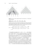
Now we can see how quickly Ak .j / grows by simply examining Ak .1/ for levels
k D 0; 1; 2; 3; 4. From the definition of A0 .k/ and the above lemmas, we have
A0 .1/ D 1 C 1 D 2, A1 .1/ D 2 1 C 1 D 3, and A2 .1/ D 21C1 .1 C 1/ 1 D 7.


574

Chapter 21 Data Structures for Disjoint Sets

We also have
A.2/
2 .1/
A2 .A2 .1//

A2 .7/
28 8 1
211 1
2047

A3 .1/ D
D
D
D
D
D
and
A4 .1/

D
D
D

A.2/
3 .1/
A3 .A3 .1//
A3 .2047/

D

.2047/
A.2048/
2
A2 .2047/
22048 2048 1

22048
.24 /512
16512
1080 ;

D
>
D
D

which is the estimated number of atoms in the observable universe. (The symbol
“ ” denotes the “much-greater-than” relation.)
We define the inverse of the function Ak .n/, for integer n 0, by
˛.n/ D min fk W Ak .1/

˚

ng :

In words, ˛.n/ is the lowest level k for which Ak .1/ is at least n. From the above
values of Ak .1/, we see that

˛.n/ D

0
1
2
3
4

for 0 Ä n Ä 2 ;
for n D 3 ;
for 4 Ä n Ä 7 ;
for 8 Ä n Ä 2047 ;
for 2048 Ä n Ä A4 .1/ :

It is only for values of n so large that the term “astronomical” understates them
(greater than A4 .1/, a huge number) that ˛.n/ > 4, and so ˛.n/ Ä 4 for all
practical purposes.


21.4 Analysis of union by rank with path compression

575

Properties of ranks
In the remainder of this section, we prove an O.m ˛.n// bound on the running time
of the disjoint-set operations with union by rank and path compression. In order to
prove this bound, we first prove some simple properties of ranks.
Lemma 21.4
For all nodes x, we have x:rank Ä x:p:rank, with strict inequality if x ¤ x:p.
The value of x:rank is initially 0 and increases through time until x ¤ x:p; from
then on, x:rank does not change. The value of x:p:rank monotonically increases
over time.
Proof The proof is a straightforward induction on the number of operations, using the implementations of M AKE -S ET, U NION, and F IND -S ET that appear in
Section 21.3. We leave it as Exercise 21.4-1.
Corollary 21.5
As we follow the simple path from any node toward a root, the node ranks strictly
increase.
Lemma 21.6

Every node has rank at most n

1.

Proof Each node’s rank starts at 0, and it increases only upon L INK operations.
Because there are at most n 1 U NION operations, there are also at most n 1
L INK operations. Because each L INK operation either leaves all ranks alone or
increases some node’s rank by 1, all ranks are at most n 1.
Lemma 21.6 provides a weak bound on ranks. In fact, every node has rank at
most blg nc (see Exercise 21.4-2). The looser bound of Lemma 21.6 will suffice
for our purposes, however.
Proving the time bound
We shall use the potential method of amortized analysis (see Section 17.3) to prove
the O.m ˛.n// time bound. In performing the amortized analysis, we will find it
convenient to assume that we invoke the L INK operation rather than the U NION
operation. That is, since the parameters of the L INK procedure are pointers to two
roots, we act as though we perform the appropriate F IND -S ET operations separately. The following lemma shows that even if we count the extra F IND -S ET operations induced by U NION calls, the asymptotic running time remains unchanged.


576

Chapter 21 Data Structures for Disjoint Sets

Lemma 21.7
Suppose we convert a sequence S 0 of m0 M AKE -S ET, U NION, and F IND -S ET operations into a sequence S of m M AKE -S ET, L INK, and F IND -S ET operations by
turning each U NION into two F IND -S ET operations followed by a L INK. Then, if
sequence S runs in O.m ˛.n// time, sequence S 0 runs in O.m0 ˛.n// time.
Proof Since each U NION operation in sequence S 0 is converted into three operations in S, we have m0 Ä m Ä 3m0 . Since m D O.m0 /, an O.m ˛.n// time bound
for the converted sequence S implies an O.m0 ˛.n// time bound for the original
sequence S 0 .

In the remainder of this section, we shall assume that the initial sequence of m0
M AKE -S ET, U NION, and F IND -S ET operations has been converted to a sequence
of m M AKE -S ET, L INK, and F IND -S ET operations. We now prove an O.m ˛.n//
time bound for the converted sequence and appeal to Lemma 21.7 to prove the
O.m0 ˛.n// running time of the original sequence of m0 operations.
Potential function
The potential function we use assigns a potential q .x/ to each node x in the
disjoint-set forest after q operations.
We sum the node potentials for the potenP
tial of the entire forest: ˆq D x q .x/, where ˆq denotes the potential of the
forest after q operations. The forest is empty prior to the first operation, and we
arbitrarily set ˆ0 D 0. No potential ˆq will ever be negative.
The value of q .x/ depends on whether x is a tree root after the qth operation.
If it is, or if x:rank D 0, then q .x/ D ˛.n/ x:rank.
Now suppose that after the qth operation, x is not a root and that x:rank
1.
We need to define two auxiliary functions on x before we can define q .x/. First
we define
level.x/ D max fk W x:p:rank

Ak .x:rank/g :

That is, level.x/ is the greatest level k for which Ak , applied to x’s rank, is no
greater than x’s parent’s rank.
We claim that
0 Ä level.x/ < ˛.n/ ;

(21.1)

which we see as follows. We have

x:p:rank

x:rank C 1 (by Lemma 21.4)
D A0 .x:rank/ (by definition of A0 .j /) ,

which implies that level.x/

0, and we have


21.4 Analysis of union by rank with path compression

A˛.n/ .x:rank/

577

A˛.n/ .1/ (because Ak .j / is strictly increasing)
n
(by the definition of ˛.n/)
> x:p:rank (by Lemma 21.6) ,

which implies that level.x/ < ˛.n/. Note that because x:p:rank monotonically
increases over time, so does level.x/.
The second auxiliary function applies when x:rank 1:
«
˚
/
.x:rank/ :
iter.x/ D max i W x:p:rank A.ilevel.x/
That is, iter.x/ is the largest number of times we can iteratively apply Alevel.x/ ,

applied initially to x’s rank, before we get a value greater than x’s parent’s rank.
We claim that when x:rank 1, we have
1 Ä iter.x/ Ä x:rank ;

(21.2)

which we see as follows. We have
x:p:rank

Alevel.x/ .x:rank/ (by definition of level.x/)
D A.1/
level.x/ .x:rank/ (by definition of functional iteration) ,

which implies that iter.x/

1, and we have

rankC1/
.x:rank/ D Alevel.x/C1 .x:rank/ (by definition of Ak .j /)
A.x:
level.x/
> x:p:rank
(by definition of level.x/) ,

which implies that iter.x/ Ä x:rank. Note that because x:p:rank monotonically
increases over time, in order for iter.x/ to decrease, level.x/ must increase. As long
as level.x/ remains unchanged, iter.x/ must either increase or remain unchanged.
With these auxiliary functions in place, we are ready to define the potential of
node x after q operations:
(

˛.n/ x:rank
if x is a root or x:rank D 0 ;
q .x/ D
.˛.n/ level.x// x:rank iter.x/ if x is not a root and x:rank 1 :
We next investigate some useful properties of node potentials.
Lemma 21.8
For every node x, and for all operation counts q, we have
0Ä

q .x/

Ä ˛.n/ x:rank :


578

Chapter 21 Data Structures for Disjoint Sets

Proof If x is a root or x:rank D 0, then q .x/ D ˛.n/ x:rank by definition. Now
suppose that x is not a root and that x:rank 1. We obtain a lower bound on q .x/
by maximizing level.x/ and iter.x/. By the bound (21.1), level.x/ Ä ˛.n/ 1, and
by the bound (21.2), iter.x/ Ä x:rank. Thus,
q .x/

D .˛.n/ level.x// x:rank iter.x/
.˛.n/ .˛.n/ 1// x:rank x:rank
D x:rank x:rank
D 0:

Similarly, we obtain an upper bound on q .x/ by minimizing level.x/ and iter.x/.

By the bound (21.1), level.x/ 0, and by the bound (21.2), iter.x/ 1. Thus,
q .x/

Ä .˛.n/ 0/ x:rank
D ˛.n/ x:rank 1
< ˛.n/ x:rank :

1

Corollary 21.9
If node x is not a root and x:rank > 0, then

q .x/

< ˛.n/ x:rank.

Potential changes and amortized costs of operations
We are now ready to examine how the disjoint-set operations affect node potentials.
With an understanding of the change in potential due to each operation, we can
determine each operation’s amortized cost.
Lemma 21.10
Let x be a node that is not a root, and suppose that the qth operation is either a
L INK or F IND -S ET. Then after the qth operation, q .x/ Ä q 1 .x/. Moreover, if
x:rank
1 and either level.x/ or iter.x/ changes due to the qth operation, then
1. That is, x’s potential cannot increase, and if it has positive
q .x/ Ä q 1 .x/
rank and either level.x/ or iter.x/ changes, then x’s potential drops by at least 1.
Proof Because x is not a root, the qth operation does not change x:rank, and
because n does not change after the initial n M AKE -S ET operations, ˛.n/ remains

unchanged as well. Hence, these components of the formula for x’s potential remain the same after the qth operation. If x:rank D 0, then q .x/ D q 1 .x/ D 0.
Now assume that x:rank 1.
Recall that level.x/ monotonically increases over time. If the qth operation
leaves level.x/ unchanged, then iter.x/ either increases or remains unchanged.
If both level.x/ and iter.x/ are unchanged, then q .x/ D q 1 .x/. If level.x/


21.4 Analysis of union by rank with path compression

579

is unchanged and iter.x/ increases, then it increases by at least 1, and so
1.
q .x/ Ä q 1 .x/
Finally, if the qth operation increases level.x/, it increases by at least 1, so that
the value of the term .˛.n/ level.x// x:rank drops by at least x:rank. Because level.x/ increased, the value of iter.x/ might drop, but according to the
bound (21.2), the drop is by at most x:rank 1. Thus, the increase in potential due to the change in iter.x/ is less than the decrease in potential due to the
change in level.x/, and we conclude that q .x/ Ä q 1 .x/ 1.
Our final three lemmas show that the amortized cost of each M AKE -S ET, L INK,
and F IND -S ET operation is O.˛.n//. Recall from equation (17.2) that the amortized cost of each operation is its actual cost plus the increase in potential due to
the operation.
Lemma 21.11
The amortized cost of each M AKE -S ET operation is O.1/.
Proof Suppose that the qth operation is M AKE -S ET .x/. This operation creates
node x with rank 0, so that q .x/ D 0. No other ranks or potentials change, and
so ˆq D ˆq 1 . Noting that the actual cost of the M AKE -S ET operation is O.1/
completes the proof.
Lemma 21.12
The amortized cost of each L INK operation is O.˛.n//.
Proof Suppose that the qth operation is L INK .x; y/. The actual cost of the L INK

operation is O.1/. Without loss of generality, suppose that the L INK makes y the
parent of x.
To determine the change in potential due to the L INK, we note that the only
nodes whose potentials may change are x, y, and the children of y just prior to the
operation. We shall show that the only node whose potential can increase due to
the L INK is y, and that its increase is at most ˛.n/:
By Lemma 21.10, any node that is y’s child just before the L INK cannot have
its potential increase due to the L INK.
From the definition of q .x/, we see that, since x was a root just before the qth
operation, q 1 .x/ D ˛.n/ x:rank. If x:rank D 0, then q .x/ D q 1 .x/ D 0.
Otherwise,
q .x/

< ˛.n/ x:rank (by Corollary 21.9)
D q 1 .x/ ;

and so x’s potential decreases.


580

Chapter 21 Data Structures for Disjoint Sets

Because y is a root prior to the L INK, q 1 .y/ D ˛.n/ y:rank. The L INK
operation leaves y as a root, and it either leaves y’s rank alone or it increases y’s
rank by 1. Therefore, either q .y/ D q 1 .y/ or q .y/ D q 1 .y/ C ˛.n/.
The increase in potential due to the L INK operation, therefore, is at most ˛.n/.
The amortized cost of the L INK operation is O.1/ C ˛.n/ D O.˛.n//.
Lemma 21.13
The amortized cost of each F IND -S ET operation is O.˛.n//.

Proof Suppose that the qth operation is a F IND -S ET and that the find path contains s nodes. The actual cost of the F IND -S ET operation is O.s/. We shall
show that no node’s potential increases due to the F IND -S ET and that at least
max.0; s .˛.n/ C 2// nodes on the find path have their potential decrease by
at least 1.
To see that no node’s potential increases, we first appeal to Lemma 21.10 for all
nodes other than the root. If x is the root, then its potential is ˛.n/ x:rank, which
does not change.
Now we show that at least max.0; s .˛.n/ C 2// nodes have their potential
decrease by at least 1. Let x be a node on the find path such that x:rank > 0
and x is followed somewhere on the find path by another node y that is not a root,
where level.y/ D level.x/ just before the F IND -S ET operation. (Node y need not
immediately follow x on the find path.) All but at most ˛.n/ C 2 nodes on the find
path satisfy these constraints on x. Those that do not satisfy them are the first node
on the find path (if it has rank 0), the last node on the path (i.e., the root), and the
last node w on the path for which level.w/ D k, for each k D 0; 1; 2; : : : ; ˛.n/ 1.
Let us fix such a node x, and we shall show that x’s potential decreases by at
least 1. Let k D level.x/ D level.y/. Just prior to the path compression caused by
the F IND -S ET, we have
.x:rank/ (by definition of iter.x/) ,
A.iter.x//
k
Ak .y:rank/
(by definition of level.y/) ,
x:p:rank
(by Corollary 21.5 and because
y follows x on the find path) .

x:p:rank
y:p:rank
y:rank

Putting these inequalities together and letting i be the value of iter.x/ before path
compression, we have
Ak .y:rank/
Ak .x:p:rank/

y:p:rank

D

(because Ak .j / is strictly increasing)

.x:rank//
Ak .A.iter.x//
k
.i C1/
Ak .x:rank/ :


21.4 Analysis of union by rank with path compression

581

Because path compression will make x and y have the same parent, we know
that after path compression, x:p:rank D y:p:rank and that the path compression
does not decrease y:p:rank. Since x:rank does not change, after path compression
we have that x:p:rank
A.ik C1/ .x:rank/. Thus, path compression will cause either iter.x/ to increase (to at least i C 1) or level.x/ to increase (which occurs if
iter.x/ increases to at least x:rank C 1). In either case, by Lemma 21.10, we have
1. Hence, x’s potential decreases by at least 1.

q .x/ Ä q 1 .x/
The amortized cost of the F IND -S ET operation is the actual cost plus the change
in potential. The actual cost is O.s/, and we have shown that the total potential
decreases by at least max.0; s .˛.n/ C 2//. The amortized cost, therefore, is at
most O.s/ .s .˛.n/ C 2// D O.s/ s C O.˛.n// D O.˛.n//, since we can
scale up the units of potential to dominate the constant hidden in O.s/.
Putting the preceding lemmas together yields the following theorem.
Theorem 21.14
A sequence of m M AKE -S ET, U NION, and F IND -S ET operations, n of which are
M AKE -S ET operations, can be performed on a disjoint-set forest with union by
rank and path compression in worst-case time O.m ˛.n//.
Proof

Immediate from Lemmas 21.7, 21.11, 21.12, and 21.13.

Exercises
21.4-1
Prove Lemma 21.4.
21.4-2
Prove that every node has rank at most blg nc.
21.4-3
In light of Exercise 21.4-2, how many bits are necessary to store x:rank for each
node x?
21.4-4
Using Exercise 21.4-2, give a simple proof that operations on a disjoint-set forest
with union by rank but without path compression run in O.m lg n/ time.
21.4-5
Professor Dante reasons that because node ranks increase strictly along a simple
path to the root, node levels must monotonically increase along the path. In other

582

Chapter 21 Data Structures for Disjoint Sets

words, if x:rank > 0 and x:p is not a root, then level.x/ Ä level.x:p/. Is the
professor correct?
21.4-6 ?
Consider the function ˛ 0 .n/ D min fk W Ak .1/ lg.n C 1/g. Show that ˛ 0 .n/ Ä 3
for all practical values of n and, using Exercise 21.4-2, show how to modify the
potential-function argument to prove that we can perform a sequence of m M AKE S ET, U NION, and F IND -S ET operations, n of which are M AKE -S ET operations, on
a disjoint-set forest with union by rank and path compression in worst-case time
O.m ˛ 0 .n//.

Problems
21-1 Off-line minimum
The off-line minimum problem asks us to maintain a dynamic set T of elements
from the domain f1; 2; : : : ; ng under the operations I NSERT and E XTRACT-M IN.
We are given a sequence S of n I NSERT and m E XTRACT-M IN calls, where each
key in f1; 2; : : : ; ng is inserted exactly once. We wish to determine which key
is returned by each E XTRACT-M IN call. Specifically, we wish to fill in an array
extractedŒ1 : : m, where for i D 1; 2; : : : ; m, extractedŒi is the key returned by
the ith E XTRACT-M IN call. The problem is “off-line” in the sense that we are
allowed to process the entire sequence S before determining any of the returned
keys.
a. In the following instance of the off-line minimum problem, each operation
I NSERT .i/ is represented by the value of i and each E XTRACT-M IN is represented by the letter E:
4; 8; E; 3; E; 9; 2; 6; E; E; E; 1; 7; E; 5 :
Fill in the correct values in the extracted array.
To develop an algorithm for this problem, we break the sequence S into homogeneous subsequences. That is, we represent S by

I1 ; E; I2 ; E; I3 ; : : : ; Im ; E; ImC1 ;
where each E represents a single E XTRACT-M IN call and each Ij represents a (possibly empty) sequence of I NSERT calls. For each subsequence Ij , we initially place
the keys inserted by these operations into a set Kj , which is empty if Ij is empty.
We then do the following:


Problems for Chapter 21

583

O FF -L INE -M INIMUM .m; n/
1 for i D 1 to n
2
determine j such that i 2 Kj
3
if j ¤ m C 1
4
extractedŒj  D i
5
let l be the smallest value greater than j
for which set Kl exists
6
Kl D Kj [ Kl , destroying Kj
7 return extracted
b. Argue that the array extracted returned by O FF -L INE -M INIMUM is correct.
c. Describe how to implement O FF -L INE -M INIMUM efficiently with a disjointset data structure. Give a tight bound on the worst-case running time of your
implementation.
21-2 Depth determination
In the depth-determination problem, we maintain a forest F D fTi g of rooted
trees under three operations:

M AKE -T REE . / creates a tree whose only node is .
F IND -D EPTH . / returns the depth of node

within its tree.

G RAFT .r; / makes node r, which is assumed to be the root of a tree, become the
child of node , which is assumed to be in a different tree than r but may or may
not itself be a root.
a. Suppose that we use a tree representation similar to a disjoint-set forest: :p
is the parent of node , except that :p D if is a root. Suppose further
that we implement G RAFT .r; / by setting r:p D and F IND -D EPTH . / by
following the find path up to the root, returning a count of all nodes other than
encountered. Show that the worst-case running time of a sequence of m M AKE T REE, F IND -D EPTH, and G RAFT operations is ‚.m2 /.
By using the union-by-rank and path-compression heuristics, we can reduce the
worst-case running time. We use the disjoint-set forest S D fSi g, where each
set Si (which is itself a tree) corresponds to a tree Ti in the forest F . The tree
structure within a set Si , however, does not necessarily correspond to that of Ti . In
fact, the implementation of Si does not record the exact parent-child relationships
but nevertheless allows us to determine any node’s depth in Ti .
The key idea is to maintain in each node a “pseudodistance” :d, which is
defined so that the sum of the pseudodistances along the simple path from to the


584

Chapter 21 Data Structures for Disjoint Sets

root of its set Si equals the depth of in Ti . That is, if the simple path from to its
root in Si is 0 ; 1 ; : : : ; k , where 0 D and k is Si ’s root, then the depth of
Pk

in Ti is j D0 j :d.
b. Give an implementation of M AKE -T REE.
c. Show how to modify F IND -S ET to implement F IND -D EPTH. Your implementation should perform path compression, and its running time should be linear
in the length of the find path. Make sure that your implementation updates
pseudodistances correctly.
d. Show how to implement G RAFT .r; /, which combines the sets containing r
and , by modifying the U NION and L INK procedures. Make sure that your
implementation updates pseudodistances correctly. Note that the root of a set Si
is not necessarily the root of the corresponding tree Ti .
e. Give a tight bound on the worst-case running time of a sequence of m M AKE T REE, F IND -D EPTH, and G RAFT operations, n of which are M AKE -T REE operations.
21-3 Tarjan’s off-line least-common-ancestors algorithm
The least common ancestor of two nodes u and in a rooted tree T is the node w
that is an ancestor of both u and and that has the greatest depth in T . In the
off-line least-common-ancestors problem, we are given a rooted tree T and an
arbitrary set P D ffu; gg of unordered pairs of nodes in T , and we wish to determine the least common ancestor of each pair in P .
To solve the off-line least-common-ancestors problem, the following procedure
performs a tree walk of T with the initial call LCA.T:root/. We assume that each
node is colored WHITE prior to the walk.
LCA.u/
1 M AKE -S ET .u/
2 F IND -S ET .u/:ancestor D u
3 for each child of u in T
4
LCA. /
5
U NION .u; /
6
F IND -S ET .u/:ancestor D u
7 u:color D BLACK
8 for each node such that fu; g 2 P

9
if :color == BLACK
10
print “The least common ancestor of”
u “and” “is” F IND -S ET . /:ancestor


Notes for Chapter 21

585

a. Argue that line 10 executes exactly once for each pair fu; g 2 P .
b. Argue that at the time of the call LCA.u/, the number of sets in the disjoint-set
data structure equals the depth of u in T .
c. Prove that LCA correctly prints the least common ancestor of u and
pair fu; g 2 P .

for each

d. Analyze the running time of LCA, assuming that we use the implementation of
the disjoint-set data structure in Section 21.3.

Chapter notes
Many of the important results for disjoint-set data structures are due at least in part
to R. E. Tarjan. Using aggregate analysis, Tarjan [328, 330] gave the first tight
upper bound in terms of the very slowly growing inverse ˛
y.m; n/ of Ackermann’s
function. (The function Ak .j / given in Section 21.4 is similar to Ackermann’s
function, and the function ˛.n/ is similar to the inverse. Both ˛.n/ and ˛
y .m; n/

are at most 4 for all conceivable values of m and n.) An O.m lg n/ upper bound
was proven earlier by Hopcroft and Ullman [5, 179]. The treatment in Section 21.4
is adapted from a later analysis by Tarjan [332], which is in turn based on an analysis by Kozen [220]. Harfst and Reingold [161] give a potential-based version of
Tarjan’s earlier bound.
Tarjan and van Leeuwen [333] discuss variants on the path-compression heuristic, including “one-pass methods,” which sometimes offer better constant factors
in their performance than do two-pass methods. As with Tarjan’s earlier analyses
of the basic path-compression heuristic, the analyses by Tarjan and van Leeuwen
are aggregate. Harfst and Reingold [161] later showed how to make a small change
to the potential function to adapt their path-compression analysis to these one-pass
variants. Gabow and Tarjan [121] show that in certain applications, the disjoint-set
operations can be made to run in O.m/ time.
Tarjan [329] showed that a lower bound of .m ˛
y.m; n// time is required for
operations on any disjoint-set data structure satisfying certain technical conditions.
This lower bound was later generalized by Fredman and Saks [113], who showed
that in the worst case, .m ˛
y.m; n// .lg n/-bit words of memory must be accessed.