Ebook Database system concepts (6th edition) Part 2
Bạn đang xem bản rút gọn của tài liệu. Xem và tải ngay bản đầy đủ của tài liệu tại đây (15.26 MB, 725 trang )
PART
4
TRANSACTION
MANAGEMENT
The term transaction refers to a collection of operations that form a single logical
unit of work. For instance, transfer of money from one account to another is a
transaction consisting of two updates, one to each account.
It is important that either all actions of a transaction be executed completely,
or, in case of some failure, partial effects of each incomplete transaction be undone. This property is called atomicity. Further, once a transaction is successfully
executed, its effects must persist in the database —a system failure should not
result in the database forgetting about a transaction that successfully completed.
This property is called durability.
In a database system where multiple transactions are executing concurrently,
if updates to shared data are not controlled there is potential for transactions
to see inconsistent intermediate states created by updates of other transactions.
Such a situation can result in erroneous updates to data stored in the database.
Thus, database systems must provide mechanisms to isolate transactions from
the effects of other concurrently executing transactions. This property is called
isolation.
Chapter 14 describes the concept of a transaction in detail, including the
properties of atomicity, durability, isolation, and other properties provided by
the transaction abstraction. In particular, the chapter makes precise the notion of
isolation by means of a concept called serializability.
Chapter 15 describes several concurrency-control techniques that help implement the isolation property. Chapter 16 describes the recovery management
component of a database, which implements the atomicity and durability properties.
Taken as a whole, the transaction-management component of a database system allows application developers to focus on the implementation of individual
transactions, ignoring the issues of concurrency and fault tolerance.
625
This page intentionally left blank
CHAPTER
14
Transactions
Often, a collection of several operations on the database appears to be a single unit
from the point of view of the database user. For example, a transfer of funds from
a checking account to a savings account is a single operation from the customer’s
standpoint; within the database system, however, it consists of several operations.
Clearly, it is essential that all these operations occur, or that, in case of a failure,
none occur. It would be unacceptable if the checking account were debited but
the savings account not credited.
Collections of operations that form a single logical unit of work are called
transactions. A database system must ensure proper execution of transactions
despite failures—either the entire transaction executes, or none of it does. Furthermore, it must manage concurrent execution of transactions in a way that
avoids the introduction of inconsistency. In our funds-transfer example, a transaction computing the customer’s total balance might see the checking-account
balance before it is debited by the funds-transfer transaction, but see the savings
balance after it is credited. As a result, it would obtain an incorrect result.
This chapter introduces the basic concepts of transaction processing. Details
on concurrent transaction processing and recovery from failures are in Chapters
15 and 16, respectively. Further topics in transaction processing are discussed in
Chapter 26.
14.1
Transaction Concept
A transaction is a unit of program execution that accesses and possibly updates
various data items. Usually, a transaction is initiated by a user program written
in a high-level data-manipulation language (typically SQL), or programming language (for example, C++, or Java), with embedded database accesses in JDBC or
ODBC. A transaction is delimited by statements (or function calls) of the form
begin transaction and end transaction. The transaction consists of all operations
executed between the begin transaction and end transaction.
This collection of steps must appear to the user as a single, indivisible unit.
Since a transaction is indivisible, it either executes in its entirety or not at all. Thus,
if a transaction begins to execute but fails for whatever reason, any changes to the
627
628
Chapter 14 Transactions
database that the transaction may have made must be undone. This requirement
holds regardless of whether the transaction itself failed (for example, if it divided
by zero), the operating system crashed, or the computer itself stopped operating.
As we shall see, ensuring that this requirement is met is difficult since some
changes to the database may still be stored only in the main-memory variables of
the transaction, while others may have been written to the database and stored
on disk. This “all-or-none” property is referred to as atomicity.
Furthermore, since a transaction is a single unit, its actions cannot appear to
be separated by other database operations not part of the transaction. While we
wish to present this user-level impression of transactions, we know that reality is
quite different. Even a single SQL statement involves many separate accesses to
the database, and a transaction may consist of several SQL statements. Therefore,
the database system must take special actions to ensure that transactions operate
properly without interference from concurrently executing database statements.
This property is referred to as isolation.
Even if the system ensures correct execution of a transaction, this serves little
purpose if the system subsequently crashes and, as a result, the system “forgets”
about the transaction. Thus, a transaction’s actions must persist across crashes.
This property is referred to as durability.
Because of the above three properties, transactions are an ideal way of structuring interaction with a database. This leads us to impose a requirement on
transactions themselves. A transaction must preserve database consistency—if a
transaction is run atomically in isolation starting from a consistent database, the
database must again be consistent at the end of the transaction. This consistency
requirement goes beyond the data integrity constraints we have seen earlier (such
as primary-key constraints, referential integrity, check constraints, and the like).
Rather, transactions are expected to go beyond that to ensure preservation of those
application-dependent consistency constraints that are too complex to state using
the SQL constructs for data integrity. How this is done is the responsibility of the
programmer who codes a transaction. This property is referred to as consistency.
To restate the above more concisely, we require that the database system
maintain the following properties of the transactions:
• Atomicity. Either all operations of the transaction are reflected properly in
the database, or none are.
• Consistency. Execution of a transaction in isolation (that is, with no other
transaction executing concurrently) preserves the consistency of the database.
• Isolation. Even though multiple transactions may execute concurrently, the
system guarantees that, for every pair of transactions Ti and Tj , it appears to Ti
that either Tj finished execution before Ti started or Tj started execution after
Ti finished. Thus, each transaction is unaware of other transactions executing
concurrently in the system.
• Durability. After a transaction completes successfully, the changes it has
made to the database persist, even if there are system failures.
14.2 A Simple Transaction Model
629
These properties are often called the ACID properties; the acronym is derived
from the first letter of each of the four properties.
As we shall see later, ensuring the isolation property may have a significant
adverse effect on system performance. For this reason, some applications compromise on the isolation property. We shall study these compromises after first
studying the strict enforcement of the ACID properties.
14.2
A Simple Transaction Model
Because SQL is a powerful and complex language, we begin our study of transactions with a simple database language that focuses on when data are moved from
disk to main memory and from main memory to disk. In doing this, we ignore
SQL insert and delete operations, and defer considering them until Section 15.8.
The only actual operations on the data are restricted in our simple language to
arithmetic operations. Later we shall discuss transactions in a realistic, SQL-based
context with a richer set of operations. The data items in our simplified model contain a single data value (a number in our examples). Each data item is identified
by a name (typically a single letter in our examples, that is, A, B, C, etc.).
We shall illustrate the transaction concept using a simple bank application
consisting of several accounts and a set of transactions that access and update
those accounts. Transactions access data using two operations:
• read(X), which transfers the data item X from the database to a variable,
also called X, in a buffer in main memory belonging to the transaction that
executed the read operation.
• write(X), which transfers the value in the variable X in the main-memory
buffer of the transaction that executed the write to the data item X in the
database.
It is important to know if a change to a data item appears only in main memory
or if it has been written to the database on disk. In a real database system, the
write operation does not necessarily result in the immediate update of the data on
the disk; the write operation may be temporarily stored elsewhere and executed
on the disk later. For now, however, we shall assume that the write operation
updates the database immediately. We shall return to this subject in Chapter 16.
Let Ti be a transaction that transfers $50 from account A to account B. This
transaction can be defined as:
Ti : read(A);
A := A − 50;
write(A);
read(B);
B := B + 50;
write(B).
630
Chapter 14 Transactions
Let us now consider each of the ACID properties. (For ease of presentation, we
consider them in an order different from the order A-C-I-D.)
• Consistency: The consistency requirement here is that the sum of A and B
be unchanged by the execution of the transaction. Without the consistency
requirement, money could be created or destroyed by the transaction! It can
be verified easily that, if the database is consistent before an execution of
the transaction, the database remains consistent after the execution of the
transaction.
Ensuring consistency for an individual transaction is the responsibility
of the application programmer who codes the transaction. This task may be
facilitated by automatic testing of integrity constraints, as we discussed in
Section 4.4.
• Atomicity: Suppose that, just before the execution of transaction Ti , the values of accounts A and B are $1000 and $2000, respectively. Now suppose
that, during the execution of transaction Ti , a failure occurs that prevents Ti
from completing its execution successfully. Further, suppose that the failure
happened after the write(A) operation but before the write(B) operation. In
this case, the values of accounts A and B reflected in the database are $950
and $2000. The system destroyed $50 as a result of this failure. In particular,
we note that the sum A + B is no longer preserved.
Thus, because of the failure, the state of the system no longer reflects
a real state of the world that the database is supposed to capture. We term
such a state an inconsistent state. We must ensure that such inconsistencies
are not visible in a database system. Note, however, that the system must at
some point be in an inconsistent state. Even if transaction Ti is executed to
completion, there exists a point at which the value of account A is $950 and the
value of account B is $2000, which is clearly an inconsistent state. This state,
however, is eventually replaced by the consistent state where the value of
account A is $950, and the value of account B is $2050. Thus, if the transaction
never started or was guaranteed to complete, such an inconsistent state would
not be visible except during the execution of the transaction. That is the reason
for the atomicity requirement: If the atomicity property is present, all actions
of the transaction are reflected in the database, or none are.
The basic idea behind ensuring atomicity is this: The database system
keeps track (on disk) of the old values of any data on which a transaction
performs a write. This information is written to a file called the log. If the
transaction does not complete its execution, the database system restores the
old values from the log to make it appear as though the transaction never
executed. We discuss these ideas further in Section 14.4. Ensuring atomicity
is the responsibility of the database system; specifically, it is handled by a
component of the database called the recovery system, which we describe in
detail in Chapter 16.
• Durability: Once the execution of the transaction completes successfully, and
the user who initiated the transaction has been notified that the transfer of
14.2 A Simple Transaction Model
631
funds has taken place, it must be the case that no system failure can result in
a loss of data corresponding to this transfer of funds. The durability property
guarantees that, once a transaction completes successfully, all the updates
that it carried out on the database persist, even if there is a system failure
after the transaction completes execution.
We assume for now that a failure of the computer system may result in loss
of data in main memory, but data written to disk are never lost. Protection
against loss of data on disk is discussed in Chapter 16. We can guarantee
durability by ensuring that either:
1. The updates carried out by the transaction have been written to disk
before the transaction completes.
2. Information about the updates carried out by the transaction and written to disk is sufficient to enable the database to reconstruct the updates
when the database system is restarted after the failure.
The recovery system of the database, described in Chapter 16, is responsible
for ensuring durability, in addition to ensuring atomicity.
• Isolation: Even if the consistency and atomicity properties are ensured for
each transaction, if several transactions are executed concurrently, their operations may interleave in some undesirable way, resulting in an inconsistent
state.
For example, as we saw earlier, the database is temporarily inconsistent
while the transaction to transfer funds from A to B is executing, with the
deducted total written to A and the increased total yet to be written to B. If a
second concurrently running transaction reads A and B at this intermediate
point and computes A+ B, it will observe an inconsistent value. Furthermore,
if this second transaction then performs updates on A and B based on the
inconsistent values that it read, the database may be left in an inconsistent
state even after both transactions have completed.
A way to avoid the problem of concurrently executing transactions is to
execute transactions serially—that is, one after the other. However, concurrent execution of transactions provides significant performance benefits, as
we shall see in Section 14.5. Other solutions have therefore been developed;
they allow multiple transactions to execute concurrently.
We discuss the problems caused by concurrently executing transactions
in Section 14.5. The isolation property of a transaction ensures that the concurrent execution of transactions results in a system state that is equivalent
to a state that could have been obtained had these transactions executed one
at a time in some order. We shall discuss the principles of isolation further in
Section 14.6. Ensuring the isolation property is the responsibility of a component of the database system called the concurrency-control system, which
we discuss later, in Chapter 15.
632
14.3
Chapter 14 Transactions
Storage Structure
To understand how to ensure the atomicity and durability properties of a transaction, we must gain a better understanding of how the various data items in the
database may be stored and accessed.
In Chapter 10 we saw that storage media can be distinguished by their relative
speed, capacity, and resilience to failure, and classified as volatile storage or
nonvolatile storage. We review these terms, and introduce another class of storage,
called stable storage.
• Volatile storage. Information residing in volatile storage does not usually
survive system crashes. Examples of such storage are main memory and
cache memory. Access to volatile storage is extremely fast, both because of
the speed of the memory access itself, and because it is possible to access any
data item in volatile storage directly.
• Nonvolatile storage. Information residing in nonvolatile storage survives
system crashes. Examples of nonvolatile storage include secondary storage
devices such as magnetic disk and flash storage, used for online storage, and
tertiary storage devices such as optical media, and magnetic tapes, used for
archival storage. At the current state of technology, nonvolatile storage is
slower than volatile storage, particularly for random access. Both secondary
and tertiary storage devices, however, are susceptible to failure which may
result in loss of information.
• Stable storage. Information residing in stable storage is never lost (never
should be taken with a grain of salt, since theoretically never cannot be
guaranteed—for example, it is possible, although extremely unlikely, that
a black hole may envelop the earth and permanently destroy all data!). Although stable storage is theoretically impossible to obtain, it can be closely
approximated by techniques that make data loss extremely unlikely. To implement stable storage, we replicate the information in several nonvolatile
storage media (usually disk) with independent failure modes. Updates must
be done with care to ensure that a failure during an update to stable storage
does not cause a loss of information. Section 16.2.1 discusses stable-storage
implementation.
The distinctions among the various storage types can be less clear in practice
than in our presentation. For example, certain systems, for example some RAID
controllers, provide battery backup, so that some main memory can survive
system crashes and power failures.
For a transaction to be durable, its changes need to be written to stable storage.
Similarly, for a transaction to be atomic, log records need to be written to stable
storage before any changes are made to the database on disk. Clearly, the degree
to which a system ensures durability and atomicity depends on how stable its
implementation of stable storage really is. In some cases, a single copy on disk is
considered sufficient, but applications whose data are highly valuable and whose
14.4 Transaction Atomicity and Durability
633
transactions are highly important require multiple copies, or, in other words, a
closer approximation of the idealized concept of stable storage.
14.4
Transaction Atomicity and Durability
As we noted earlier, a transaction may not always complete its execution successfully. Such a transaction is termed aborted. If we are to ensure the atomicity
property, an aborted transaction must have no effect on the state of the database.
Thus, any changes that the aborted transaction made to the database must be
undone. Once the changes caused by an aborted transaction have been undone,
we say that the transaction has been rolled back. It is part of the responsibility of
the recovery scheme to manage transaction aborts. This is done typically by maintaining a log. Each database modification made by a transaction is first recorded
in the log. We record the identifier of the transaction performing the modification,
the identifier of the data item being modified, and both the old value (prior to
modification) and the new value (after modification) of the data item. Only then
is the database itself modified. Maintaining a log provides the possibility of redoing a modification to ensure atomicity and durability as well as the possibility of
undoing a modification to ensure atomicity in case of a failure during transaction
execution. Details of log-based recovery are discussed in Chapter 16.
A transaction that completes its execution successfully is said to be committed. A committed transaction that has performed updates transforms the database
into a new consistent state, which must persist even if there is a system failure.
Once a transaction has committed, we cannot undo its effects by aborting
it. The only way to undo the effects of a committed transaction is to execute a
compensating transaction. For instance, if a transaction added $20 to an account,
the compensating transaction would subtract $20 from the account. However, it
is not always possible to create such a compensating transaction. Therefore, the
responsibility of writing and executing a compensating transaction is left to the
user, and is not handled by the database system. Chapter 26 includes a discussion
of compensating transactions.
We need to be more precise about what we mean by successful completion
of a transaction. We therefore establish a simple abstract transaction model. A
transaction must be in one of the following states:
•
•
•
•
Active, the initial state; the transaction stays in this state while it is executing.
Partially committed, after the final statement has been executed.
Failed, after the discovery that normal execution can no longer proceed.
Aborted, after the transaction has been rolled back and the database has been
restored to its state prior to the start of the transaction.
• Committed, after successful completion.
The state diagram corresponding to a transaction appears in Figure 14.1. We
say that a transaction has committed only if it has entered the committed state.
634
Chapter 14 Transactions
partially
commiĴed
commiĴed
failed
aborted
active
Figure 14.1 State diagram of a transaction.
Similarly, we say that a transaction has aborted only if it has entered the aborted
state. A transaction is said to have terminated if it has either committed or aborted.
A transaction starts in the active state. When it finishes its final statement, it
enters the partially committed state. At this point, the transaction has completed
its execution, but it is still possible that it may have to be aborted, since the actual
output may still be temporarily residing in main memory, and thus a hardware
failure may preclude its successful completion.
The database system then writes out enough information to disk that, even in
the event of a failure, the updates performed by the transaction can be re-created
when the system restarts after the failure. When the last of this information is
written out, the transaction enters the committed state.
As mentioned earlier, we assume for now that failures do not result in loss of
data on disk. Chapter 16 discusses techniques to deal with loss of data on disk.
A transaction enters the failed state after the system determines that the
transaction can no longer proceed with its normal execution (for example, because
of hardware or logical errors). Such a transaction must be rolled back. Then, it
enters the aborted state. At this point, the system has two options:
• It can restart the transaction, but only if the transaction was aborted as a
result of some hardware or software error that was not created through the
internal logic of the transaction. A restarted transaction is considered to be a
new transaction.
• It can kill the transaction. It usually does so because of some internal logical
error that can be corrected only by rewriting the application program, or
because the input was bad, or because the desired data were not found in the
database.
We must be cautious when dealing with observable external writes, such as
writes to a user’s screen, or sending email. Once such a write has occurred, it
cannot be erased, since it may have been seen external to the database system.
14.5 Transaction Isolation
635
Most systems allow such writes to take place only after the transaction has entered
the committed state. One way to implement such a scheme is for the database
system to store any value associated with such external writes temporarily in
a special relation in the database, and to perform the actual writes only after
the transaction enters the committed state. If the system should fail after the
transaction has entered the committed state, but before it could complete the
external writes, the database system will carry out the external writes (using the
data in nonvolatile storage) when the system is restarted.
Handling external writes can be more complicated in some situations. For
example, suppose the external action is that of dispensing cash at an automated
teller machine, and the system fails just before the cash is actually dispensed (we
assume that cash can be dispensed atomically). It makes no sense to dispense
cash when the system is restarted, since the user may have left the machine. In
such a case a compensating transaction, such as depositing the cash back in the
user’s account, needs to be executed when the system is restarted.
As another example, consider a user making a booking over the Web. It is
possible that the database system or the application server crashes just after the
booking transaction commits. It is also possible that the network connection to
the user is lost just after the booking transaction commits. In either case, even
though the transaction has committed, the external write has not taken place.
To handle such situations, the application must be designed such that when the
user connects to the Web application again, she will be able to see whether her
transaction had succeeded or not.
For certain applications, it may be desirable to allow active transactions to
display data to users, particularly for long-duration transactions that run for
minutes or hours. Unfortunately, we cannot allow such output of observable
data unless we are willing to compromise transaction atomicity. In Chapter 26,
we discuss alternative transaction models that support long-duration, interactive
transactions.
14.5
Transaction Isolation
Transaction-processing systems usually allow multiple transactions to run concurrently. Allowing multiple transactions to update data concurrently causes
several complications with consistency of the data, as we saw earlier. Ensuring
consistency in spite of concurrent execution of transactions requires extra work;
it is far easier to insist that transactions run serially—that is, one at a time, each
starting only after the previous one has completed. However, there are two good
reasons for allowing concurrency:
• Improved throughput and resource utilization. A transaction consists of
many steps. Some involve I/O activity; others involve CPU activity. The CPU
and the disks in a computer system can operate in parallel. Therefore, I/O
activity can be done in parallel with processing at the CPU. The parallelism
636
Chapter 14 Transactions
of the CPU and the I/O system can therefore be exploited to run multiple
transactions in parallel. While a read or write on behalf of one transaction
is in progress on one disk, another transaction can be running in the CPU,
while another disk may be executing a read or write on behalf of a third
transaction. All of this increases the throughput of the system—that is, the
number of transactions executed in a given amount of time. Correspondingly,
the processor and disk utilization also increase; in other words, the processor
and disk spend less time idle, or not performing any useful work.
• Reduced waiting time. There may be a mix of transactions running on a
system, some short and some long. If transactions run serially, a short transaction may have to wait for a preceding long transaction to complete, which
can lead to unpredictable delays in running a transaction. If the transactions
are operating on different parts of the database, it is better to let them run
concurrently, sharing the CPU cycles and disk accesses among them. Concurrent execution reduces the unpredictable delays in running transactions.
Moreover, it also reduces the average response time: the average time for a
transaction to be completed after it has been submitted.
The motivation for using concurrent execution in a database is essentially the
same as the motivation for using multiprogramming in an operating system.
When several transactions run concurrently, the isolation property may be violated, resulting in database consistency being destroyed despite the correctness
of each individual transaction. In this section, we present the concept of schedules to help identify those executions that are guaranteed to ensure the isolation
property and thus database consistency.
The database system must control the interaction among the concurrent transactions to prevent them from destroying the consistency of the database. It does so
through a variety of mechanisms called concurrency-control schemes. We study
concurrency-control schemes in Chapter 15; for now, we focus on the concept of
correct concurrent execution.
Consider again the simplified banking system of Section 14.1, which has
several accounts, and a set of transactions that access and update those accounts.
Let T1 and T2 be two transactions that transfer funds from one account to another.
Transaction T1 transfers $50 from account A to account B. It is defined as:
T1 : read(A);
A := A − 50;
write(A);
read(B);
B := B + 50;
write(B).
Transaction T2 transfers 10 percent of the balance from account A to account B. It
is defined as:
14.5 Transaction Isolation
637
TRENDS IN CONCURRENCY
Several current trends in the field of computing are giving rise to an increase
in the amount of concurrency possible. As database systems exploit this concurrency to increase overall system performance, there will necessarily be an
increasing number of transactions run concurrently.
Early computers had only one processor. Therefore, there was never any real
concurrency in the computer. The only concurrency was apparent concurrency
created by the operating system as it shared the processor among several distinct
tasks or processes. Modern computers are likely to have many processors. These
may be truly distinct processors all part of the one computer. However even a
single processor may be able to run more than one process at a time by having
multiple cores. The Intel Core Duo processor is a well-known example of such a
multicore processor.
For database systems to take advantage of multiple processors and multiple
cores, two approaches are being taken. One is to find parallelism within a single
transaction or query. Another is to support a very large number of concurrent
transactions.
Many service providers now use large collections of computers rather than
large mainframe computers to provide their services. They are making this
choice based on the lower cost of this approach. A result of this is yet a further
increase in the degree of concurrency that can be supported.
The bibliographic notes refer to texts that describe these advances in computer architecture and parallel computing. Chapter 18 describes algorithms for
building parallel database systems, which exploit multiple processors and multiple cores.
T2 : read(A);
temp := A * 0.1;
A := A − temp;
write(A);
read(B);
B := B + temp;
write(B).
Suppose the current values of accounts A and B are $1000 and $2000, respectively. Suppose also that the two transactions are executed one at a time in the
order T1 followed by T2 . This execution sequence appears in Figure 14.2. In the
figure, the sequence of instruction steps is in chronological order from top to
bottom, with instructions of T1 appearing in the left column and instructions of
T2 appearing in the right column. The final values of accounts A and B, after the
execution in Figure 14.2 takes place, are $855 and $2145, respectively. Thus, the
total amount of money in accounts A and B—that is, the sum A + B—is preserved
after the execution of both transactions.
638
Chapter 14 Transactions
T1
T2
read(A)
A := A − 50
write(A)
read(B)
B := B + 50
write(B)
commit
read(A)
temp := A ∗ 0.1
A := A − temp
write(A)
read(B)
B := B + temp
write(B)
commit
Figure 14.2 Schedule 1—a serial schedule in which T1 is followed by T2 .
Similarly, if the transactions are executed one at a time in the order T2 followed
by T1 , then the corresponding execution sequence is that of Figure 14.3. Again, as
expected, the sum A + B is preserved, and the final values of accounts A and B
are $850 and $2150, respectively.
T1
T2
read(A)
temp := A ∗ 0.1
A := A − temp
write(A)
read(B)
B := B + temp
write(B)
commit
read(A)
A := A − 50
write(A)
read(B)
B := B + 50
write(B)
commit
Figure 14.3 Schedule 2—a serial schedule in which T2 is followed by T1 .
14.5 Transaction Isolation
639
The execution sequences just described are called schedules. They represent
the chronological order in which instructions are executed in the system. Clearly,
a schedule for a set of transactions must consist of all instructions of those transactions, and must preserve the order in which the instructions appear in each
individual transaction. For example, in transaction T1 , the instruction write(A)
must appear before the instruction read(B), in any valid schedule. Note that we
include in our schedules the commit operation to indicate that the transaction
has entered the committed state. In the following discussion, we shall refer to
the first execution sequence (T1 followed by T2 ) as schedule 1, and to the second
execution sequence (T2 followed by T1 ) as schedule 2.
These schedules are serial: Each serial schedule consists of a sequence of
instructions from various transactions, where the instructions belonging to one
single transaction appear together in that schedule. Recalling a well-known formula from combinatorics, we note that, for a set of n transactions, there exist n
factorial (n!) different valid serial schedules.
When the database system executes several transactions concurrently, the
corresponding schedule no longer needs to be serial. If two transactions are
running concurrently, the operating system may execute one transaction for a
little while, then perform a context switch, execute the second transaction for
some time, and then switch back to the first transaction for some time, and so on.
With multiple transactions, the CPU time is shared among all the transactions.
Several execution sequences are possible, since the various instructions from
both transactions may now be interleaved. In general, it is not possible to predict
exactly how many instructions of a transaction will be executed before the CPU
switches to another transaction.1
Returning to our previous example, suppose that the two transactions are
executed concurrently. One possible schedule appears in Figure 14.4. After this
execution takes place, we arrive at the same state as the one in which the transactions are executed serially in the order T1 followed by T2 . The sum A + B is indeed
preserved.
Not all concurrent executions result in a correct state. To illustrate, consider
the schedule of Figure 14.5. After the execution of this schedule, we arrive at a
state where the final values of accounts A and B are $950 and $2100, respectively.
This final state is an inconsistent state, since we have gained $50 in the process of
the concurrent execution. Indeed, the sum A + B is not preserved by the execution
of the two transactions.
If control of concurrent execution is left entirely to the operating system, many
possible schedules, including ones that leave the database in an inconsistent state,
such as the one just described, are possible. It is the job of the database system to
ensure that any schedule that is executed will leave the database in a consistent
state. The concurrency-control component of the database system carries out this
task.
1 The number of possible schedules for a set of n transactions is very large. There are n! different serial schedules.
Considering all the possible ways that steps of transactions might be interleaved, the total number of possible schedules
is much larger than n!.
640
Chapter 14 Transactions
T1
T2
read(A)
A := A − 50
write(A)
read(A)
temp := A ∗ 0.1
A := A − temp
write(A)
read(B)
B := B + 50
write(B)
commit
read(B)
B := B + temp
write(B)
commit
Figure 14.4 Schedule 3—a concurrent schedule equivalent to schedule 1.
We can ensure consistency of the database under concurrent execution by
making sure that any schedule that is executed has the same effect as a schedule
that could have occurred without any concurrent execution. That is, the schedule
should, in some sense, be equivalent to a serial schedule. Such schedules are
called serializable schedules.
T1
T2
read(A)
A := A − 50
read(A)
temp := A ∗ 0.1
A := A − temp
write(A)
read(B)
write(A)
read(B)
B := B + 50
write(B)
commit
B := B + temp
write(B)
commit
Figure 14.5 Schedule 4—a concurrent schedule resulting in an inconsistent state.
14.6 Serializability
14.6
641
Serializability
Before we can consider how the concurrency-control component of the database
system can ensure serializability, we consider how to determine when a schedule
is serializable. Certainly, serial schedules are serializable, but if steps of multiple
transactions are interleaved, it is harder to determine whether a schedule is serializable. Since transactions are programs, it is difficult to determine exactly what
operations a transaction performs and how operations of various transactions interact. For this reason, we shall not consider the various types of operations that a
transaction can perform on a data item, but instead consider only two operations:
read and write. We assume that, between a read(Q) instruction and a write(Q)
instruction on a data item Q, a transaction may perform an arbitrary sequence of
operations on the copy of Q that is residing in the local buffer of the transaction.
In this model, the only significant operations of a transaction, from a scheduling
point of view, are its read and write instructions. Commit operations, though
relevant, are not considered until Section 14.7. We therefore may show only read
and write instructions in schedules, as we do for schedule 3 in Figure 14.6.
In this section, we discuss different forms of schedule equivalence, but focus
on a particular form called conflict serializability.
Let us consider a schedule S in which there are two consecutive instructions,
I and J , of transactions Ti and Tj , respectively (i = j). If I and J refer to different
data items, then we can swap I and J without affecting the results of any instruction in the schedule. However, if I and J refer to the same data item Q, then the
order of the two steps may matter. Since we are dealing with only read and write
instructions, there are four cases that we need to consider:
1. I = read(Q), J = read(Q). The order of I and J does not matter, since the
same value of Q is read by Ti and Tj , regardless of the order.
2. I = read(Q), J = write(Q). If I comes before J , then Ti does not read the value
of Q that is written by Tj in instruction J . If J comes before I , then Ti reads
the value of Q that is written by Tj . Thus, the order of I and J matters.
T1
T2
read(A)
write(A)
read(A)
write(A)
read(B)
write(B)
read(B)
write(B)
Figure 14.6 Schedule 3—showing only the read and write instructions.
642
Chapter 14 Transactions
T1
T2
read(A)
write(A)
read(A)
read(B)
write(A)
write(B)
read(B)
write(B)
Figure 14.7 Schedule 5—schedule 3 after swapping of a pair of instructions.
3. I = write(Q), J = read(Q). The order of I and J matters for reasons similar
to those of the previous case.
4. I = write(Q), J = write(Q). Since both instructions are write operations, the
order of these instructions does not affect either Ti or Tj . However, the value
obtained by the next read(Q) instruction of S is affected, since the result of
only the latter of the two write instructions is preserved in the database. If
there is no other write(Q) instruction after I and J in S, then the order of I
and J directly affects the final value of Q in the database state that results
from schedule S.
Thus, only in the case where both I and J are read instructions does the relative
order of their execution not matter.
We say that I and J conflict if they are operations by different transactions
on the same data item, and at least one of these instructions is a write operation.
To illustrate the concept of conflicting instructions, we consider schedule 3in
Figure 14.6. The write(A) instruction of T1 conflicts with the read(A) instruction
of T2 . However, the write(A) instruction of T2 does not conflict with the read(B)
instruction of T1 , because the two instructions access different data items.
T1
T2
read(A)
write(A)
read(B)
write(B)
read(A)
write(A)
read(B)
write(B)
Figure 14.8 Schedule 6—a serial schedule that is equivalent to schedule 3.
14.6 Serializability
T3
643
T4
read(Q)
write(Q)
write(Q)
Figure 14.9 Schedule 7.
Let I and J be consecutive instructions of a schedule S. If I and J are instructions of different transactions and I and J do not conflict, then we can swap
the order of I and J to produce a new schedule S . S is equivalent to S , since all
instructions appear in the same order in both schedules except for I and J , whose
order does not matter.
Since the write(A) instruction of T2 in schedule 3 of Figure 14.6 does not conflict
with the read(B) instruction of T1 , we can swap these instructions to generate an
equivalent schedule, schedule 5, in Figure 14.7. Regardless of the initial system
state, schedules 3 and 5 both produce the same final system state.
We continue to swap nonconflicting instructions:
• Swap the read(B) instruction of T1 with the read(A) instruction of T2 .
• Swap the write(B) instruction of T1 with the write(A) instruction of T2 .
• Swap the write(B) instruction of T1 with the read(A) instruction of T2 .
The final result of these swaps, schedule 6 of Figure 14.8, is a serial schedule.
Note that schedule 6 is exactly the same as schedule 1, but it shows only the
read and write instructions. Thus, we have shown that schedule 3 is equivalent
to a serial schedule. This equivalence implies that, regardless of the initial system
state, schedule 3 will produce the same final state as will some serial schedule.
If a schedule S can be transformed into a schedule S by a series of swaps of
nonconflicting instructions, we say that S and S are conflict equivalent.2
Not all serial schedules are conflict equivalent to each other. For example,
schedules 1 and 2 are not conflict equivalent.
The concept of conflict equivalence leads to the concept of conflict serializability. We say that a schedule S is conflict serializable if it is conflict equivalent
to a serial schedule. Thus, schedule 3 is conflict serializable, since it is conflict
equivalent to the serial schedule 1.
Finally, consider schedule 7 of Figure 14.9; it consists of only the significant
operations (that is, the read and write) of transactions T3 and T4 . This schedule
is not conflict serializable, since it is not equivalent to either the serial schedule
<T3 ,T4 > or the serial schedule <T4 ,T3 >.
2 We use the term conflict equivalent to distinguish the way we have just defined equivalence from other definitions that
we shall discuss later on in this section.
644
Chapter 14 Transactions
T1
T2
T2
(a)
T1
(b)
Figure 14.10 Precedence graph for (a) schedule 1 and (b) schedule 2.
We now present a simple and efficient method for determining conflict serializability of a schedule. Consider a schedule S. We construct a directed graph,
called a precedence graph, from S. This graph consists of a pair G = (V, E), where
V is a set of vertices and E is a set of edges. The set of vertices consists of all the
transactions participating in the schedule. The set of edges consists of all edges
Ti → Tj for which one of three conditions holds:
1. Ti executes write(Q) before Tj executes read(Q).
2. Ti executes read(Q) before Tj executes write(Q).
3. Ti executes write(Q) before Tj executes write(Q).
If an edge Ti → Tj exists in the precedence graph, then, in any serial schedule S
equivalent to S, Ti must appear before Tj .
For example, the precedence graph for schedule 1 in Figure 14.10a contains
the single edge T1 → T2 , since all the instructions of T1 are executed before the
first instruction of T2 is executed. Similarly, Figure 14.10b shows the precedence
graph for schedule 2 with the single edge T2 → T1 , since all the instructions of T2
are executed before the first instruction of T1 is executed.
The precedence graph for schedule 4 appears in Figure 14.11. It contains
the edge T1 → T2 , because T1 executes read(A) before T2 executes write(A). It also
contains the edge T2 → T1 , because T2 executes read(B) before T1 executes write(B).
If the precedence graph for S has a cycle, then schedule S is not conflict serializable. If the graph contains no cycles, then the schedule S is conflict serializable.
A serializability order of the transactions can be obtained by finding a linear
order consistent with the partial order of the precedence graph. This process is
called topological sorting. There are, in general, several possible linear orders that
T1
T2
Figure 14.11 Precedence graph for schedule 4.
14.6 Serializability
645
Ti
Tk
Tj
Tm
(a)
Ti
Ti
Tj
Tk
Tk
Tj
Tm
Tm
(b)
(c)
Figure 14.12 Illustration of topological sorting.
can be obtained through a topological sort. For example, the graph of Figure 14.12a
has the two acceptable linear orderings shown in Figures 14.12b and 14.12c.
Thus, to test for conflict serializability, we need to construct the precedence
graph and to invoke a cycle-detection algorithm. Cycle-detection algorithms can
be found in standard textbooks on algorithms. Cycle-detection algorithms, such
as those based on depth-first search, require on the order of n2 operations, where
n is the number of vertices in the graph (that is, the number of transactions).
Returning to our previous examples, note that the precedence graphs for
schedules 1 and 2 (Figure 14.10) indeed do not contain cycles. The precedence
graph for schedule 4 (Figure 14.11), on the other hand, contains a cycle, indicating
that this schedule is not conflict serializable.
It is possible to have two schedules that produce the same outcome, but that
are not conflict equivalent. For example, consider transaction T5 , which transfers
$10 from account B to account A. Let schedule 8 be as defined in Figure 14.13.
We claim that schedule 8 is not conflict equivalent to the serial schedule <T1 ,T5 >,
since, in schedule 8, the write(B) instruction of T5 conflicts with the read(B) instruction of T1 . This creates an edge T5 → T1 in the precedence graph. Similarly,
we see that the write(A) instruction of T1 conflicts with the read instruction of T5
646
Chapter 14 Transactions
T1
T5
read(A)
A := A − 50
write(A)
read(B)
B := B − 10
write(B)
read(B)
B := B + 50
write(B)
read(A)
A := A + 10
write(A)
Figure 14.13 Schedule 8.
creating an edge T1 → T5 . This shows that the precedence graph has a cycle and
that schedule 8 is not serializable. However, the final values of accounts A and
B after the execution of either schedule 8 or the serial schedule <T1 ,T5 > are the
same—$960 and $2040, respectively.
We can see from this example that there are less-stringent definitions of schedule equivalence than conflict equivalence. For the system to determine that schedule 8 produces the same outcome as the serial schedule <T1 ,T5 >, it must analyze
the computation performed by T1 and T5 , rather than just the read and write operations. In general, such analysis is hard to implement and is computationally
expensive. In our example, the final result is the same as that of a serial schedule
because of the mathematical fact that addition and subtraction are commutative.
While this may be easy to see in our simple example, the general case is not so
easy since a transaction may be expressed as a complex SQL statement, a Java
program with JDBC calls, etc.
However, there are other definitions of schedule equivalence based purely on
the read and write operations. One such definition is view equivalence, a definition
that leads to the concept of view serializability. View serializability is not used in
practice due to its high degree of computational complexity.3 We therefore defer
discussion of view serializability to Chapter 15, but, for completeness, note here
that the example of schedule 8 is not view serializable.
14.7
Transaction Isolation and Atomicity
So far, we have studied schedules while assuming implicitly that there are no
transaction failures. We now address the effect of transaction failures during
concurrent execution.
3 Testing
for view serializability has been proven to be NP-complete, which means that it is virtually certain that no
efficient test for view serializability exists.
14.7 Transaction Isolation and Atomicity
T6
647
T7
read(A)
write(A)
read(A)
commit
read(B)
Figure 14.14 Schedule 9, a nonrecoverable schedule.
If a transaction Ti fails, for whatever reason, we need to undo the effect of
this transaction to ensure the atomicity property of the transaction. In a system
that allows concurrent execution, the atomicity property requires that any transaction Tj that is dependent on Ti (that is, Tj has read data written by Ti ) is also
aborted. To achieve this, we need to place restrictions on the type of schedules
permitted in the system.
In the following two subsections, we address the issue of what schedules are
acceptable from the viewpoint of recovery from transaction failure. We describe
in Chapter 15 how to ensure that only such acceptable schedules are generated.
14.7.1
Recoverable Schedules
Consider the partial schedule 9 in Figure 14.14, in which T7 is a transaction that
performs only one instruction: read(A). We call this a partial schedule because
we have not included a commit or abort operation for T6 . Notice that T7 commits
immediately after executing the read(A) instruction. Thus, T7 commits while T6
is still in the active state. Now suppose that T6 fails before it commits. T7 has read
the value of data item A written by T6 . Therefore, we say that T7 is dependent
on T6 . Because of this, we must abort T7 to ensure atomicity. However, T7 has
already committed and cannot be aborted. Thus, we have a situation where it is
impossible to recover correctly from the failure of T6 .
Schedule 9 is an example of a nonrecoverable schedule. A recoverable schedule
is one where, for each pair of transactions Ti and Tj such that Tj reads a data item
previously written by Ti , the commit operation of Ti appears before the commit
operation of Tj . For the example of schedule 9 to be recoverable, T7 would have
to delay committing until after T6 commits.
14.7.2
Cascadeless Schedules
Even if a schedule is recoverable, to recover correctly from the failure of a transaction Ti , we may have to roll back several transactions. Such situations occur if
transactions have read data written by Ti . As an illustration, consider the partial
schedule of Figure 14.15. Transaction T8 writes a value of A that is read by transaction T9 . Transaction T9 writes a value of A that is read by transaction T10 . Suppose
that, at this point, T8 fails. T8 must be rolled back. Since T9 is dependent on T8 , T9
must be rolled back. Since T10 is dependent on T9 , T10 must be rolled back. This
648
Chapter 14 Transactions
T8
T9
T10
read(A)
read(B)
write(A)
read(A)
write(A)
read(A)
abort
Figure 14.15 Schedule 10.
phenomenon, in which a single transaction failure leads to a series of transaction
rollbacks, is called cascading rollback.
Cascading rollback is undesirable, since it leads to the undoing of a significant
amount of work. It is desirable to restrict the schedules to those where cascading
rollbacks cannot occur. Such schedules are called cascadeless schedules. Formally,
a cascadeless schedule is one where, for each pair of transactions Ti and Tj such
that Tj reads a data item previously written by Ti , the commit operation of Ti
appears before the read operation of Tj . It is easy to verify that every cascadeless
schedule is also recoverable.
14.8
Transaction Isolation Levels
Serializability is a useful concept because it allows programmers to ignore issues
related to concurrency when they code transactions. If every transaction has the
property that it maintains database consistency if executed alone, then serializability ensures that concurrent executions maintain consistency. However, the
protocols required to ensure serializability may allow too little concurrency for
certain applications. In these cases, weaker levels of consistency are used. The
use of weaker levels of consistency places additional burdens on programmers
for ensuring database correctness.
The SQL standard also allows a transaction to specify that it may be executed in
such a way that it becomes nonserializable with respect to other transactions. For
instance, a transaction may operate at the isolation level of read uncommitted,
which permits the transaction to read a data item even if it was written by a
transaction that has not been committed. SQL provides such features for the
benefit of long transactions whose results do not need to be precise. If these
transactions were to execute in a serializable fashion, they could interfere with
other transactions, causing the others’ execution to be delayed.
The isolation levels specified by the SQL standard are as follows:
• Serializable usually ensures serializable execution. However, as we shall
explain shortly, some database systems implement this isolation level in a
manner that may, in certain cases, allow nonserializable executions.
14.8 Transaction Isolation Levels
649
• Repeatable read allows only committed data to be read and further requires
that, between two reads of a data item by a transaction, no other transaction
is allowed to update it. However, the transaction may not be serializable
with respect to other transactions. For instance, when it is searching for data
satisfying some conditions, a transaction may find some of the data inserted
by a committed transaction, but may not find other data inserted by the same
transaction.
• Read committed allows only committed data to be read, but does not require
repeatable reads. For instance, between two reads of a data item by the transaction, another transaction may have updated the data item and committed.
• Read uncommitted allows uncommitted data to be read. It is the lowest
isolation level allowed by SQL.
All the isolation levels above additionally disallow dirty writes, that is, they
disallow writes to a data item that has already been written by another transaction
that has not yet committed or aborted.
Many database systems run, by default, at the read-committed isolation level.
In SQL, it is possible to set the isolation level explicitly, rather than accepting the
system’s default setting. For example, the statement “set transaction isolation
level serializable;” sets the isolation level to serializable; any of the other isolation levels may be specified instead. The above syntax is supported by Oracle,
PostgreSQL and SQL Server; DB2 uses the syntax “change isolation level,” with its
own abbreviations for isolation levels.
Changing of the isolation level must be done as the first statement of a
transaction. Further, automatic commit of individual statements must be turned
off, if it is on by default; API functions, such as the JDBC method Connection.setAutoCommit(false) which we saw in Section 5.1.1.7, can be used to do
so. Further, in JDBC the method Connection.setTransactionIsolation(int level) can
be used to set the isolation level; see the JDBC manuals for details.
An application designer may decide to accept a weaker isolation level in order
to improve system performance. As we shall see in Section 14.9 and Chapter 15,
ensuring serializability may force a transaction to wait for other transactions or,
in some cases, to abort because the transaction can no longer be executed as
part of a serializable execution. While it may seem shortsighted to risk database
consistency for performance, this trade-off makes sense if we can be sure that the
inconsistency that may occur is not relevant to the application.
There are many means of implementing isolation levels. As long as the implementation ensures serializability, the designer of a database application or a
user of an application does not need to know the details of such implementations,
except perhaps for dealing with performance issues. Unfortunately, even if the
isolation level is set to serializable, some database systems actually implement a
weaker level of isolation, which does not rule out every possible nonserializable
execution; we revisit this issue in Section 14.9. If weaker levels of isolation are
used, either explicitly or implicitly, the application designer has to be aware of
some details of the implementation, to avoid or minimize the chance of inconsistency due to lack of serializability.