Ebook The finite element method (2nd edition) Part 1
Bạn đang xem bản rút gọn của tài liệu. Xem và tải ngay bản đầy đủ của tài liệu tại đây (1.35 MB, 181 trang )
The Finite Element Method
This page intentionally left blank
The Finite Element Method
An Introduction with Partial Differential
Equations
Second Edition
A. J. DAVIES
Professor of Mathematics
University of Hertfordshire
1
3
Great Clarendon Street, Oxford ox2 6dp
Oxford University Press is a department of the University of Oxford.
It furthers the University’s objective of excellence in research, scholarship,
and education by publishing worldwide in
Oxford New York
Auckland Cape Town Dar es Salaam Hong Kong Karachi
Kuala Lumpur Madrid Melbourne Mexico City Nairobi
New Delhi Shanghai Taipei Toronto
With offices in
Argentina Austria Brazil Chile Czech Republic France Greece
Guatemala Hungary Italy Japan Poland Portugal Singapore
South Korea Switzerland Thailand Turkey Ukraine Vietnam
Oxford is a registered trade mark of Oxford University Press
in the UK and in certain other countries
Published in the United States
by Oxford University Press Inc., New York
c A. J. Davies 2011
The moral rights of the author have been asserted
Database right Oxford University Press (maker)
First Edition published 1980
Second Edition published 2011
All rights reserved. No part of this publication may be reproduced,
stored in a retrieval system, or transmitted, in any form or by any means,
without the prior permission in writing of Oxford University Press,
or as expressly permitted by law, or under terms agreed with the appropriate
reprographics rights organization. Enquiries concerning reproduction
outside the scope of the above should be sent to the Rights Department,
Oxford University Press, at the address above
You must not circulate this book in any other binding or cover
and you must impose the same condition on any acquirer
British Library Cataloguing in Publication Data
Data available
Library of Congress Cataloging in Publication Data
Data available
Typeset by SPI Publisher Services, Pondicherry, India
Printed in Great Britain by
Ashford Colour Press Ltd, Gosport, Hampshire
ISBN 978–0–19–960913–0
1 3 5 7 9 10 8 6 4 2
Preface
In the first paragraph of the preface to the first edition in 1980 I wrote:
It is not easy, for the newcomer to the subject, to get into the current finite element
literature. The purpose of this book is to offer an introductory approach, after which
the well-known texts should be easily accessible.
Writing now, in 2010, I feel that this is still largely the case. However, while the
1980 text was probably the only introductory text at that time, it is not the case
now. I refer the interested reader to the references.
In this second edition, I have maintained the general ethos of the first.
It is primarily a text for mathematicians, scientists and engineers who have
no previous experience of finite elements. It has been written as an undergraduate text but will also be useful to postgraduates. It is also suitable for
anybody already using large finite element or CAD/CAM packages and who
would like to understand a little more of what is going on. The main aim is
to provide an introduction to the finite element solution of problems posed as
partial differential equations. It is self-contained in that it requires no previous
knowledge of the subject. Familiarity with the mathematics normally covered by
the end of the second year of undergraduate courses in mathematics, physical
science or engineering is all that is assumed. In particular, matrix algebra
and vector calculus are used extensively throughout; the necessary theorems from
vector calculus are collected together in Appendix B.
The reader familiar with the first edition will notice some significant changes.
I now present the method as a numerical technique for the solution of partial
differential equations, comparable with the finite difference method. This is
in contrast to the first edition, in which the technique was developed as an
extension of the ideas of structural analysis. The only thing that remains of this
approach is the terminology, for example ‘stiffness matrix’, since this is still in
common parlance. The reader familiar with the first edition will notice a change
in notation which reflects the move away from the structural background. There
is also a change of order of chapters: the introduction to finite elements is now
via weighted residual methods, variational methods being delayed until later.
I have taken the opportunity to introduce a completely new chapter on boundary
element methods. At the time of the first edition, such methods were in their
infancy, but now they have reached such a stage of development that it is natural
to include them; this chapter is by no means exhaustive and is very much an
introduction. I have also included a brief chapter on computational aspects. This
is also an introduction; the topic is far too large to treat in any depth. Again
the interested reader can follow up the references. In the first edition, many of
vi
The Finite Element Method
the examples and exercises were based on problems in journal papers of around
that time. I have kept the original references in this second edition.
In Chapter 1, I have written an updated historical introduction and included
many new references. Chapter 2 provides a background in weighted residual
and variational methods. Chapter 3 describes the finite element method for
Poisson’s equation, concentrating on linear elements. Higher-order elements and
the isoparametric concept are introduced in Chapter 4.
Chapter 5 sets the finite element method in a variational context and introduces time-dependent and non-linear problems. Chapter 6 is almost identical
with Chapter 7 of the first edition, the only change being the notation. Chapter
7 is the new chapter on the boundary element method, and Chapter 8, the
final chapter, addresses the computational aspects. I have also expanded the
appendices by including, in Appendix A, a brief description of some of the
partial differential equation models in the physical sciences which are amenable
to solution by the finite element method.
I have not changed the general approach of the first edition. At the end of
each chapter is a set of exercises with detailed solutions. They serve two purposes:
(i) to give the reader the opportunity to practice the techniques, and (ii) to
develop the theory a little further where this does not require any new concepts;
for example, the finite element solution of eigenvalue problems is considered in
Exercise 3.24. Also, some of the basic theory of Chapter 6 is left to the exercises.
Consequently, certain results of importance are to be found in the exercises and
their solutions.
An important development over the past thirty years has been the wide
availability of computational aids such as spreadsheets and computer algebra
packages. In this edition, I have included examples of how a spreadsheet could
be used to develop more sophisticated solutions compared with the ‘hand’
calculations in the first edition. Obviously, I would encourage readers to use
whichever packages they have on their own personal computers.
Well, this second edition has been a long time coming; I’ve been working
on it for quite some time. It has been confined to very concentrated two-week
spells over the Easter periods for the past six years, these periods being spent
with Margaret and Arthur, Les Meuniers, at their home in the Lot, south-west
France. The environment there is ideal for the sort of focused work needed to
produce this second edition. I am grateful for their friendship and, of course, their
hospitality. The production of this edition would have been impossible without
the help of Dr Diane Crann, my wife. I am very grateful for her expertise in
turning my sometimes illegible handwritten script into OUP LATEX house style.
A.J.D.
Lacombrade
Sabadel Latronqui`ere
Lot
August 2010
Contents
1
Historical introduction
2
Weighted residual and variational methods
2.1 Classification of differential operators
2.2 Self-adjoint positive definite operators
2.3 Weighted residual methods
2.4 Extremum formulation: homogeneous boundary
conditions
2.5 Non-homogeneous boundary conditions
2.6 Partial differential equations: natural boundary
conditions
2.7 The Rayleigh–Ritz method
2.8 The ‘elastic analogy’ for Poisson’s equation
2.9 Variational methods for time-dependent problems
2.10 Exercises and solutions
3
4
The finite element method for elliptic problems
3.1 Difficulties associated with the application of weighted
residual methods
3.2 Piecewise application of the Galerkin method
3.3 Terminology
3.4 Finite element idealization
3.5 Illustrative problem involving one independent variable
3.6 Finite element equations for Poisson’s equation
3.7 A rectangular element for Poisson’s equation
3.8 A triangular element for Poisson’s equation
3.9 Exercises and solutions
Higher-order elements: the isoparametric concept
4.1 A two-point boundary-value problem
4.2 Higher-order rectangular elements
4.3 Higher-order triangular elements
4.4 Two degrees of freedom at each node
4.5 Condensation of internal nodal freedoms
4.6 Curved boundaries and higher-order elements: isoparametric
elements
4.7 Exercises and solutions
1
7
7
9
12
24
28
32
35
44
48
50
71
71
72
73
75
80
91
102
107
114
141
141
144
145
147
151
153
160
viii
5
The Finite Element Method
Further topics in the finite element method
5.1 The variational approach
5.2 Collocation and least squares methods
5.3 Use of Galerkin’s method for time-dependent and non-linear
problems
5.4 Time-dependent problems using variational principles which
are not extremal
5.5 The Laplace transform
5.6 Exercises and solutions
171
171
177
6
Convergence of the finite element method
6.1 A one-dimensional example
6.2 Two-dimensional problems involving Poisson’s equation
6.3 Isoparametric elements: numerical integration
6.4 Non-conforming elements: the patch test
6.5 Comparison with the finite difference method: stability
6.6 Exercises and solutions
218
218
224
226
228
229
234
7
The
7.1
7.2
7.3
7.4
7.5
7.6
244
244
247
251
256
259
261
8
Computational aspects
8.1 Pre-processor
8.2 Solution phase
8.3 Post-processor
8.4 Finite element method (FEM) or boundary element method
(BEM)?
boundary element method
Integral formulation of boundary-value problems
Boundary element idealization for Laplace’s equation
A constant boundary element for Laplace’s equation
A linear element for Laplace’s equation
Time-dependent problems
Exercises and solutions
179
189
192
199
270
270
271
274
274
Appendix A Partial differential equation models in the physical
sciences
A.1 Parabolic problems
A.2 Elliptic problems
A.3 Hyperbolic problems
A.4 Initial and boundary conditions
276
276
277
278
279
Appendix B Some integral theorems of the vector calculus
280
Appendix C A formula for integrating products of area coordinates
over a triangle
282
Contents
Appendix
D.1
D.2
D.3
D Numerical integration formulae
One-dimensional Gauss quadrature
Two-dimensional Gauss quadrature
Logarithmic Gauss quadrature
ix
284
284
284
285
Appendix E Stehfest’s formula and weights for numerical Laplace
transform inversion
287
References
288
Index
295
This page intentionally left blank
1
Historical introduction
The fundamental idea of the finite element method is the replacement of continuous functions by piecewise appproximations, usually polynomials.
Although the finite element method itself is relatively new, its development
and success expanding with the arrival and rapid growth of the digital computer,
the idea of piecewise approximation is far from new. Indeed, the early geometers
used ‘finite elements’ to determine an approximate value of π. They did this
by bounding a quadrant of a circle with inscribed and circumscribed polygons,
the straight-line segments being the finite element approximations to an arc of
the circle. In this way, they were able to obtain extremely accurate estimates.
Upper and lower bounds were obtained, and by taking an increasing number of
elements, monotonic convergence to the exact solution would be expected. These
phenomena are also possible in modern applications of the finite element method.
One remark regarding ancient finite elements: Archimedes used these ideas to
determine areas of plane figures and volumes of solids, although of course he did
not have a precise concept of a limiting procedure. Indeed, it was only this fact
which prevented him from discovering the integral calculus some two thousand
years before Newton and Leibniz. The interesting point here is that whilst many
problems of applied mathematics are posed in terms of differential equations,
the finite element solution of such equations uses ideas which are in fact much
older than those used to set up the equations initially.
The modern use of finite elements really started in the field of structural
engineering. Probably the first attempts were by Hrennikoff (1941) and McHenry
(1943), who developed analogies between actual discrete elements, for example
bars and beams, and the corresponding portions of a continuous solid. These
methods belonged to a class of semi-analytic techniques which were used in the
1940s for aircraft structural design. Matrix methods for the solution of such
problems were developed at this time, and it is interesting to note that the
work of Argyris (1955), in an engineering context, introduced a minimization
process which is also the basis of the mathematical underpinning of the finite
element method. With the development of high-speed, jet-powered aircraft,
these semi-analytic methods were soon found to be inadequate and the quest
began for a more reliable approach. A direct approach, based on the principle
of virtual work, was given by Argyris (1955), and in a series of papers he
and his colleagues developed this work to solve very complex problems using
computational techniques (Argyris and Kelsey 1960). At about the same time,
2
The Finite Element Method
Turner et al. (1956) presented the element stiffness matrix, based on displacement
assumptions, for a triangular element, together with the direct stiffness method
for assembling the elements. The term ‘finite element’ was introduced by Clough
(1960) in a paper describing applications in plane elasticity.
The engineers had put the finite element method on the map as a practical
technique for solving their elasticity problems, and although a rigorous mathematical basis had not been developed, the next few years saw an expansion
of the method to solve a large variety of structural problems. Solutions of
three-dimensional problems required only simple extensions to the basic twodimensional theory (Argyris 1964). The obvious problem to consider after plane
problems was that of plate bending; here, researchers found their first real
difficulties and the early attempts were not altogether successful. It was not
until some time later that the problems of compatibility were resolved (Bazely
et al. 1965).
One area of application of plate elements was that of modelling thin shells,
and some success was achieved (Clough and Johnson 1968). However, the representation of a thin shell by a polyhedral surface of flat plates can cause serious
problems in the presence of pronounced bending, and it soon became clear that
shell elements themselves were necessary.
Plate elements presented difficulties to researchers, but these were small
compared with the problems associated with shell elements. The first actual shell
elements developed were axisymmetric elements (Grafton and Strome 1963), and
these were followed by a whole sequence of cylindrical and other shell elements
(Gallagher 1969). Such elements are still being developed, and it is probably fair
to say that this is the only area of linear analysis that still has potential for
further work in the context of finite elements.
The workers in the early 1960s soon turned their attention towards the
solution of non-linear problems. Turner et al. (1960) showed how to use an
incremental technique to solve geometrically non-linear problems, i.e. problems in
which the strains remain small but displacements are large. Stability analysis also
comes into this category and was discussed by Martin (1965). Plasticity problems,
involving non-linear material behaviour, were modelled at this time (Gallagher
et al. 1962) and the method was also applied to the solution of problems in
viscoelasticity (Zienkiewicz et al. 1968).
Besides the static analysis described above, dynamic problems were also
being tackled, and Archer (1963) introduced the concept of the consistent mass
matrix. Both vibration problems (Zienkiewicz et al. 1966) and transient problems
(Koenig and Davids 1969) were considered. Thus the period from its conception
in the early 1950s to the late 1960s saw the method being applied extensively by
the engineering community. With the successes of these practical applications in
the structural field, it was open for engineers in other disciplines (Silvester and
Historical introduction
3
Ferrari 1983) to get hold of the finite element method. An obvious candidate was
fluid mechanics.
Potential flow (Doctors 1970) and Stokes flow were easy to develop
(Atkinson et al. 1970), and it wasn’t long before the appearance of a textbook on
the finite element method in viscous flow problems (Connor and Brebbia 1976).
However, the more general form of the Navier–Stokes equations was much more
difficult, the convection terms yield non-self-adjoint operators and, consequently,
there are no obvious variational principles. The method was extended further
when it was seen to fit in with the method of weighted residuals (Szab´
o and
Lee 1969). This then allowed the solution of such problems posed as partial
differential equation boundary-value problems. The method had been well known
for some time; Crandall (1956) had used the term to classify a variety of
numerical approximation techniques, although Galerkin (1915) was the first to
use the method. Probably the first finite element solution of the Navier–Stokes
equations was given by Taylor and Hood (1973). However, problems that had
been encountered using finite differences (Spalding 1972) were apparent in the
finite element approach, and the so-called up-wind approach was brought into
a finite element context (Zienkiewicz, Heinrich et al. 1977). Also, the so-called
finite-volume approach was developed (Jameson and Mavriplis 1986), which has
the important physical property that certain conservation laws are maintained.
The scene was now set for rapid developments in fluid mechanics and other areas
such as heat and mass transfer (Mohr 1992), for diffusion–convection problems,
and for other coupled problems (Elliott and Larsson 1995).
As far as this historical introduction is concerned, this is where we shall
leave the contributions from the engineering community. There are excellent
accounts of applications from the mid 1970s onwards in the texts by Zienkiewicz
and Taylor (2000a,b). Let us return to the early days of the developments: at
the same time as the engineers were pushing forward with the practical aspects
of the method, similar work was being carried out by applied mathematicians,
each group apparently unaware of the work of the other. Courant (1943) gave
a solution to the torsion problem, using piecewise linear approximations over
a triangular mesh, formulating the problem from the principle of minimum
potential energy. Zienkiewicz (1995) noted that Courant had already developed
some of the ideas in the 1920s without taking them further. Similar papers
followed by Polya (1952) and Weinberger (1956). Greenstadt (1959) presented
the idea of considering a continuous region as an assembly of several discrete
parts and making assumptions about the variables in each region, variational
principles being used to find values for these variables. We note here also that
the work of Schoenberg (1946) was very much in the spirit of finite elements, since
the piecewise polynomial approximation led to the development of the theory of
splines.
4
The Finite Element Method
Similar work was being carried out in the physics community. In the late
1940s, Prager and Synge (1947) developed a geometric approach to a variational
principle in elasticity which led to the so-called hypercircle method, which is also
in the spirit of the finite element method. The method is discussed in detail in
the book by Synge (1957). A three-dimensional problem in electrostatics was
solved, using linear tetrahedral elements, by McMahon (1953).
It was some time before Birkhoff et al. (1968) and Zlamal (1968) published
a convergence proof and error bounds in the applied mathematics literature.
However, the first convergence proof in the engineering literature had already
been given by Melosh (1963), who used the principle of minimum potential
energy, and this work was extended by Jones (1964) using Reissner’s variational
principle. Once it was realized that the method could be interpreted in terms of
variational methods, the mathematicians and engineers were brought together
and many extensions of the method to new areas soon followed. In particular,
it was realized that the concept of piecewise polynomial approximation offered
a simple and efficient procedure for the application of the classical Rayleigh–
Ritz method. The principles could be clearly seen in the much earlier work
of Lord Rayleigh (Strutt 1870) and Ritz (1909). From a physical point of
view, it meant that problems outside the structural area could be solved using
standard structural packages by associating suitable meanings to the terms in the
corresponding variational principles. This was just what was done by Zienkiewicz
and Cheung (1965) in the application of the finite element method to the solution
of Poisson’s equation and by Doctors (1970) in the application to potential flow.
Similarly, transient heat conduction problems were considered by Wilson and
Nickell (1966).
The mathematical basis of the method then started in earnest, and it is
well beyond the scope of this text to do more than indicate where the interested
reader may wish to start. Error estimation is clearly an important aspect of any
numerical approximation, and the first developments were by Babuˇska (1971,
1973) and Babuˇska and Rheinboldt (1978, 1979), who showed how to estimate
errors and how convergence was ensured by suitable mesh refinement. The basis
was then set for the possibility of adaptive mesh refinement, in which meshes
are automatically refined in response to knowledge of computed solutions. Mesh
generation and adaption is an area in which much work is still needed; for a
recent account, see Zienkiewicz et al. (2005). Ciarlet (1978) provided the first of
what would usually be described as a ‘mathematical’ account of the finite element
method, and the text has since been extended and updated by Ciarlet and Lions
(1991). The reader interested in becoming familiar with current mathematical
approaches to the method should consult Brenner and Scott (1994) or the very
readable text by Axelsson and Barker (2001).
At about the same time as Courant was working on variational methods for elliptic problems, Trefftz (1926) developed a technique in which a
Historical introduction
5
partial differential equation, defined over a region, becomes an integral equation
over the boundary of that region. The immediate advantage is in the reduction
of the dimension of the problem. Such integral techniques have been known since
the late nineteenth century; the theorems of Green (1828) are the bedrock of the
solution of potential problems, the term potential first being coined by Green in
his seminal paper. These techniques have been the basis of the formulation of
potential theory and elasticity by, amongst others, Fredholm (1903) and Kellog
(1929).
It was with developments in computing and numerical procedures that the
technique became attractive to physicists and engineers in the 1960s (Hess and
Smith 1964), and the ideas developed at that time were collected together in
a single text (Jaswon and Symm 1977). A very good overview of the early
development of boundary elements was given by Becker (1992). It is interesting
to note here the work of Rizzo (1967), who applied the ideas for potential
problems to use boundary elements to solve problems in elasticity, in contrast
with Zienkiewicz and Cheung (1965), who used codes for structural analysis to
obtain the finite element solution of potential problems.
The first boundary element textbook was written by Brebbia (1978), and
since then there has been a variety of similar texts, each with the intention
of making the technique accessible to those who would wish to develop their
own code. See, for example, Gipson (1987), Becker (1992) and Par´ıs and Ca˜
nas
(1997). The text by Hall (1993) is particularly useful to those for whom boundary
elements are a completely new idea. Finally, the two-volume set by Aliabadi
(2002) and Wrobel (2002) provides a similar state-of-the-art work on boundary
elements, as does the three-volume set by Zienkiewicz and Taylor (2000a,b) and
Zienkiewicz et al. (2005) for finite elements.
There is always the question ‘Which is better, the finite element method or
the boundary element method?’ See Chapter 8, where we discuss the merits of
each case. It is usually accepted that boundary elements are more appropriate
for infinite regions. However, in a recent text, Wolf and Song (1997) set out
a finite element procedure to cope with unbounded regions. Zienkiewicz, Kelly
et al. (1977) proposed a coupling of the two methods to get the best out of each:
finite elements in regions of material non-linearity and boundary elements for
unbounded regions.
Recently, further developments in so-called mesh-free methods have been
proposed (Goldberg and Chen 1997, Liu 2003); included is the method of
fundamental solutions (Goldberg and Chen 1999), which has its origins in the
work on potential problems by Kupradze (1965).
Currently, the terms ‘finite element method’, ‘boundary element method’,
‘mesh-free method’ etc. are used, and they are all really variations on a more
general weighted residual theme. Zienkiewicz (1995) suggested that a more
appropriate generic name would be the generalized Galerkin method (Fletcher
6
The Finite Element Method
1984). For further details of background and history, see the following: for finite
elements, Zienkiewicz (1995) and Fish and Belytschko (2007), who gave a very
good account of the commercial development of finite elements; and for boundary
elements, see Becker (1992) and Cheng and Cheng (2005). There is now a very
large body of work in the finite element method field; a quick Internet search on
the words ‘finite element’ and ‘boundary element’ yielded more than 20 million
pages. The website run at the University of Ohio gives details of more than 600
finite element books.
The finite element method has now reached a very sophisticated level
of development, so much so that it is applied routinely in a wide variety of
application areas. We mention here just two of them. (i) Biomedical engineering: Zienkiewicz (1977) performed stress analysis calculations for human femur
transplants. Recently, Phillips (2009) has extended these ideas significantly and,
instead of modelling just the bone, he has made a complete finite element analysis
of the bone and the associated muscles. (ii) Financial engineering: in the early
days of the development of finite elements, the study of financial systems would
have seemed to have been outside the scope of the method. However, Black–
Scholes models (Wilmott et al. 1995), describing a variety of option-pricing
schemes, have been set in a finite element context by, amongst others, Topper
(2005) and Tao Jiang et al. (2009).
For a general guide to current research from both an engineering and
a mathematical perspective, the reader is referred to the sets of conference
proceedings MAFELAP (From 1973 to 2010), edited by Whiteman, and BEM
(From 1979 to 2010), edited by Brebbia.
Finally, if there is one person whose work forms a basis for both the finite
element method and the boundary element method then it is George Green.
Green’s theorem underpins both methods, and, of course, fundamental solutions
are themselves Green’s functions.
2
2.1
Weighted residual and variational
methods
Classification of differential operators
The quantities of interest in many areas of applied mathematics are often to
be found as the solution of certain partial differential equations, together with
prescribed boundary and/or initial conditions.
The nature of the solution of a partial differential equation depends on the
form that the equation takes. All linear, and quasi-linear, second-order equations
are classified as elliptic, hyperbolic or parabolic. In each of these categories there
are equations which model certain physical phenomena. The classification is
determined by the coefficients of the highest partial derivatives which occur in
the equation.
In this chapter, we shall consider functions which depend on two independent variables only, so that the resulting algebra does not obscure the underlying
ideas.
Consider the second-order partial differential equation
Lu = f,
(2.1)
where L is the operator defined by
Lu ≡ a
∂2u
∂2u
∂2u
+
c
+
b
+F
∂x2
∂x∂y
∂ 2 y2
x, y, u,
∂u ∂u
,
.
∂x ∂y
a, b and c are, in general, functions of x and y; they may also depend on u itself
and its derivatives, in which case the equation is non-linear. Non-linear equations
are, in general, far more difficult to deal with than linear equations, and they will
not be discussed here. They will, however, be considered briefly in Section 5.3.
Equation (2.1) is said to be:
• elliptic if b2 < 4ac;
• hyperbolic if b2 > 4ac;
• parabolic if b2 = 4ac.
Unlike ordinary differential equations, it is not usually profitable to investigate
the solution of a partial differential equation in isolation from the associated
boundary and/or initial conditions. Indeed, it will always be an equation together
8
The Finite Element Method
with prescribed conditions which forms a mathematical model of a particular
situation.
In general, elliptic equations are associated with steady-state phenomena
and require a knowledge of values of the unknown function, or its derivative, on
the boundary of the region of interest. Thus Poisson’s equation,
−∇2 u =
ρ
,
gives a model which describes the variation of the electrostatic potential in a
medium with permittivity and in which there is a charge distribution ρ per
unit volume. In the case ρ ≡ 0 we have Laplace’s equation,
∇2 u = 0.
In order that the solution is unique, it is necessary to know the potential or
charge distribution on the surrounding boundary. This is a pure boundary-value
problem.
Hyperbolic equations are, in general, associated with propagation problems
and require the specification of certain initial values and/or possible boundary
values as well.
Thus, the wave equation,
1 ∂2u
∂2u
= 2 2,
2
∂x
c ∂t
gives the small transverse displacement, u(x, t), of a uniform vibrating string;
waves are propagated along the string with speed c. In such problems it is usually
required to know the displacement, or its derivative, at the ends, together with
the initial displacement and velocity distribution. This is an initial boundaryvalue problem.
Finally, parabolic equations model problems in which the quantity of interest
varies slowly in comparison with the random motions which produce these
variations. As is the case with hyperbolic equations, they are associated with
initial-value problems. Thus the heat equation, or diffusion equation,
1 ∂u
∂2u
,
=
2
∂x
α ∂t
describes the temperature variation, u(x, t), in a thin rod which has a uniform
thermal diffusivity α. The temperature changes in the material are produced by
the motion of individual molecules and occur slowly in comparison with these
molecular motions. Either the temperature or its derivative is usually given at
the ends of the rod, together with an initial temperature distribution. This again
is an initial boundary-value problem. The three equations occur in many areas
of applied mathematics, engineering and science. In Appendix A we provide a
Weighted residual and variational methods
9
table of application areas, so that the interested reader may be able to associate
the equations with appropriate applications.
In this chapter we shall consider the approximate methods on which our
finite element techniques, described in Chapters 3, 4, 5 and 6, will be based. It
is in the area of elliptic partial differential equations that finite element methods
have been used most extensively, since the differential operators involved belong
to the important class of positive definite operators. However, finite elements
are widely used for the solution of hyperbolic and parabolic equations, and all
three categories will be discussed; elliptic equations in Chapters 3 and 4, and
hyperbolic and parabolic equations in Chapter 5.
2.2
Self-adjoint positive definite operators
Suppose that the function u satisfies eqn (2.1) in a two-dimensional region D
bounded by a closed curve C, i.e.
Lu = f,
where f (x, y) is a given function of position. Suppose also that u satisfies certain
given homogeneous conditions on the boundary C. Usually these conditions are
of the following types:
(2.2)
Dirichlet boundary condition: u = 0;
(2.3)
(2.4)
Neumann condition:
Robin condition:
∂u
= 0;
∂n
∂u
+ σ(s)u = 0.
∂n
Here s is the arc length measured along C from some fixed point on C, and ∂/∂n
represents differentiation along the outward normal to the boundary. Note that
the Neumann condition may be obtained from the Robin condition by setting
σ ≡ 0.
A problem is said to be properly posed, in the sense of Hadamard (1923), if
and only if the following conditions hold:
1. A solution exists.
2. The solution is unique.
3. The solution depends continuously on the data.
The third condition is equivalent to saying that small changes in the data lead
to small changes in the solution (Renardy and Rogers 1993). If at least one of
10
The Finite Element Method
these conditions does not hold, then the problem is said to be poorly posed or
ill-posed.
For an elliptic operator L, the problem is properly posed only when one of
these conditions holds at each point on the boundary.
The numerical methods which we shall discuss involve processes which
change our partial differential equation into a system of linear algebraic equations. Two important properties of L lead to particularly useful properties of the
system matrix.
1. The operator L is said to be self-adjoint if and only if the expression
vLu dx dy −
uLv dx dy
D
D
is a function only of u, v and their derivatives evaluated on the boundary.
In particular, for homogeneous boundary conditions, L is self-adjoint if and
only if
vLu dx dy =
uLv dx dy.
D
D
2. The operator L is said to be positive definite if and only if, for all functions u,
uLu dx dy ≥ 0,
D
equality occurring if and only if u ≡ 0.
In both definitions, it is assumed that u and v satisfy suitable differentiability
conditions in order that the operations exist.
Example 2.1 Suppose that L = −∇2 , so that eqn (2.1) becomes Poisson’s equation; then
vLu dx dy −
D
u ∇2 v dx dy −
uLv dx dy =
D
v ∇2 u dx dy
D
=
u
C
∂u
∂v
−v
∂n
∂n
D
ds
by virtue of the second form of Green’s theorem. Thus the operator −∇2 is
self-adjoint.
Also, v ∇2 u = div (v grad u) − grad u · grad v, and thus
u −∇2 u dx dy = −
D
| grad u |2 dx dy
div (u grad u) dx dy +
D
D
Weighted residual and variational methods
=−
u
C
∂u
ds +
∂n
11
| grad u |2 dx dy,
D
using the divergence theorem; see Appendix B.
Thus if u satisfies either of the boundary conditions (2.2) or (2.3) it follows
that −∇2 is positive definite. For the Robin boundary condition (2.4), the
boundary integral becomes
σu2 ds
C
2
and hence −∇ is positive definite provided that σ > 0.
Example 2.2 Suppose now that Lu = −div (k grad u), where k (x, y) is a scalar
function of position, and suppose also that the problem is isotropic. Anisotropy
can be taken into account by replacing the scalar k by a tensor represented by
κ=
(2.5)
κxx κxy
;
κyx κyy
see eqn (2.68).
vLu dx dy −
D
uLv dx dy
D
u div (k grad v) dx dy −
=
D
v div (k grad u) dx dy
D
{div (uk grad v) − grad u · k grad v} dx dy
=
D
−
{div (vk grad u) − grad v · k grad u} dx dy
D
k u
=
C
∂u
∂v
−v
∂u
∂n
ds
∂u
ds +
∂n
k | grad u |2 dx dy.
using the divergence theorem.
Hence L is self-adjoint. Also,
uLu dx dy = −
D
ku
C
If u satisfies eqn (2.2) or eqn (2.3), then the boundary integral vanishes and L
is positive definite if k > 0. If, however, u satisfies eqn (2.4), then the boundary
integral is negative if σ > 0, so that again L is positive definite if k > 0.
12
The Finite Element Method
When one is modelling physical phenomena, an important property that
the model must possess is that it has a unique solution. If the physical system
is modelled by eqn (2.1) and L is linear and positive definite, then the solution
is unique. The proof is as follows.
Suppose that u1 and u2 are two solutions of eqn (2.1). Let
v = u1 − u2 ,
so that
Lv = Lu1 − Lu2 = 0.
Hence
vLv dx dy = 0.
D
Now L is positive definite, so that v ≡ 0. Thus u1 = u2 and the solution is unique.
2.3
Weighted residual methods
Consider the boundary-value problem
Lu = f
(2.6)
in
D
subject to the non-homogeneous Dirichlet boundary condition
u = g(s)
on some part C1 of the boundary, and the non-homogeneous Robin condition
∂u
+ σ(s)u = h(s)
∂n
on the remainder C2 .
An approximate solution u
˜ will not, in general, satisfy eqn (2.6) exactly, and
associated with such an approximate solution is the residual defined by
r(˜
u) = L˜
u − f.
If the exact solution is u0 , then
r(u0 ) ≡ 0.
13
Weighted residual and variational methods
We choose a set of basis functions {vi : i = 0, . . . , n}, and make an approximation of the following form:
n
u
˜n =
(2.7)
ci vi .
i=0
In the weighted residual method, the unknown parameters ci are chosen to
minimize the residual r(˜
u) in some sense. Different methods of minimizing the
residual yield different approximate solutions.
All the methods we shall consider result in a system of equations of the form
Ac = h
for the unknowns ci . The different methods yield different matrices A and h.
The methods presented in this section are illustrated in Examples 2.3–2.6,
in which all calculations are done by hand. A comparison of these solutions with
the exact solution is shown in Table 2.1 and Fig. 2.1. We shall consider the simple
two-point boundary-value problem
0 < x < 1,
−u = x2 ,
u(0) = u(1) = 0.
(2.8)
This problem has the exact solution
u0 (x) =
x
1 − x3 .
12
Example 2.3 Firstly, consider the collocation method, in which the trial function
(2.7) is chosen to satisfy the boundary conditions.
N.B. We choose homogeneous Dirichlet boundary conditions. Onedimensional problems with non-homogeneous conditions of the form u(0) = a,
u(1) = b may be transformed to a problem with homogeneous conditions by the
change of dependent variable w(x) = u(x) − ((1 − x)a + xb).
˜n to satisfy the differential
The parameters ci are then found by forcing u
equation at a given set of n points, i.e. at these points the residual vanishes.
Table 2.1 Approximate solutions (×102 ) to the boundary-value problem
of Examples 2.3–2.6
x
0
0.2
0.4
0.6
0.8
1
Collocation
Overdetermined collocation
Least squares
Galerkin
Exact
0
0
0
0
0
1.422
1.533
1.867
1.600
1.653
2.933
3.100
3.600
3.200
3.120
3.733
3.900
4.400
4.000
3.920
3.022
3.133
3.467
3.200
3.253
0
0
0
0
0
14
The Finite Element Method
Absolute errors (×103)
5.5
Collocation
Overdetermined collocation
Least squares
Galerkin
5
4.5
4
3.5
3
2.5
2
1.5
1
0.5
0
0
0.2
0.4
0.6
0.8
1
x
Fig. 2.1 Comparison of the errors in the four approximate solutions in Examples 2.3–2.6.
The residual is
r (˜
un ) = − u
˜n + x2 .
A cubic approximation which satisfies the boundary conditions is
u
˜1 (x) = x(1 − x)(c0 + c1 x),
so that
r (˜
u1 ) = 2c0 + (6x − 2)c1 − x2 .
If x =
1
3
and x =
2
3
are chosen as collocation points, then
r u
˜1
1
3
=r u
˜1
2
3
= 0,
which leads to the equations
20
22
c0
c1
=
1
9
4
9
,
1
giving c0 = 18
, c1 = 16 .
Thus the approximate solution is
u
˜1 (x) =
1
x(1 − x)(1 + 3x).
18