Ebook ASCI alliance center for simulation of dynamic response in materials FY 2000 annual report Part 1
Bạn đang xem bản rút gọn của tài liệu. Xem và tải ngay bản đầy đủ của tài liệu tại đây (6.5 MB, 51 trang )
CALTECH ASCI TECHNICAL REPORT 076
caltechASCI/2000.076
ASCI Alliance Center for Simulation of Dynamic Response in Materials
California Institute of Technology
FY 2000 Annual Report
Michael Aivazis, Bill Goddard, Dan Meiron, Michael Ortiz,
James C.T. Pool, Joe Shepherd, Principal Investigators
ASCI Alliance Center
for
Simulation of Dynamic
Response in Materials
California Insitute of
Technology
FY 2000 Annual Report
Michael Aivazis, Bill Goddard, Dan Meiron, Michael Ortiz, James
C. T. Pool, Joe Shepherd
Principal Investigators
Contents
1
2
3
4
5
Introduction and Overview
1.1 Introduction . . . . . . . . . . . . . . . . . . .
1.2 Administration of the Center . . . . . . . . . .
1.3 Overview of the integrated simulation capability
1.4 Highlights of Research Accomplishments . . .
.
.
.
.
.
.
.
.
.
.
.
.
.
.
.
.
.
.
.
.
.
.
.
.
.
.
.
.
.
.
.
.
.
.
.
.
.
.
.
.
.
.
.
.
.
.
.
.
1
1
2
3
4
Integrated Simulation Capability
2.1 Introduction . . . . . . . . .
2.2 Algorithmic integration . . .
2.3 Fluid dynamics algorithms .
2.4 Solid Mechanics algorithms
2.5 Software integration . . . . .
.
.
.
.
.
.
.
.
.
.
.
.
.
.
.
.
.
.
.
.
.
.
.
.
.
.
.
.
.
.
.
.
.
.
.
.
.
.
.
.
.
.
.
.
.
.
.
.
.
.
.
.
.
.
.
.
.
.
.
.
.
.
.
.
.
.
.
.
.
.
.
.
.
.
.
8
8
8
14
20
22
High Explosives
3.1 Overview of FY00 Accomplishments . . .
3.2 Personnel . . . . . . . . . . . . . . . . . .
3.3 Material Properties and Chemical Reactions
3.4 Engineering Models of Explosives . . . . .
3.5 Eulerian-Lagrangian Coupling Algorithms .
3.6 Reduced Reaction Modeling . . . . . . . .
.
.
.
.
.
.
.
.
.
.
.
.
.
.
.
.
.
.
.
.
.
.
.
.
.
.
.
.
.
.
.
.
.
.
.
.
.
.
.
.
.
.
.
.
.
.
.
.
.
.
.
.
.
.
.
.
.
.
.
.
.
.
.
.
.
.
.
.
.
.
.
.
.
.
.
.
.
.
.
.
.
.
.
.
28
28
29
29
30
31
33
Solid Dynamics
4.1 Overview of FY 00 Accomplishments
4.2 Personnel . . . . . . . . . . . . . . .
4.3 Nanomechanics . . . . . . . . . . . .
4.4 Mesomechanics . . . . . . . . . . . .
4.5 Macromechanics . . . . . . . . . . .
4.6 Polymorphic Phase Transitions . . . .
4.7 Eulerian Elastic-Plastic Solver . . . .
4.8 FY 01 objectives . . . . . . . . . . .
.
.
.
.
.
.
.
.
.
.
.
.
.
.
.
.
.
.
.
.
.
.
.
.
.
.
.
.
.
.
.
.
.
.
.
.
.
.
.
.
.
.
.
.
.
.
.
.
.
.
.
.
.
.
.
.
.
.
.
.
.
.
.
.
.
.
.
.
.
.
.
.
.
.
.
.
.
.
.
.
.
.
.
.
.
.
.
.
.
.
.
.
.
.
.
.
.
.
.
.
.
.
.
.
.
.
.
.
.
.
.
.
48
48
48
49
52
54
59
60
64
Materials Properties
5.1 Overview of FY 00 Accomplishments . . . . . . . . . . . . . . . . .
5.2 Personnel . . . . . . . . . . . . . . . . . . . . . . . . . . . . . . . .
71
71
72
.
.
.
.
.
.
.
.
.
.
.
.
.
.
.
i
.
.
.
.
.
.
.
.
.
.
.
.
.
.
.
.
.
.
.
.
.
.
.
.
.
.
.
.
.
.
.
.
.
.
.
.
.
.
.
.
.
.
.
.
CONTENTS
5.3
5.4
5.5
6
7
ii
Materials properties for high explosives . . . . . . . . . . . . . . . .
Materials Properties for Solid Dynamics . . . . . . . . . . . . . . . .
Materials properties methodology development . . . . . . . . . . . .
73
76
80
Compressible Turbulence
6.1 Introduction . . . . . . . . . . . . . . . . . . . . . .
6.2 Overview of FY 00 Accomplishments . . . . . . . .
6.3 Personnel . . . . . . . . . . . . . . . . . . . . . . .
6.4 Pseudo-DNS of Richtmyer-Meshkov instability . . .
6.5 LES of Richtmyer-Meshkov instability . . . . . . . .
6.6 Implementation of CFD Euler solvers within GrACE
6.7 DNS of Rayleigh-Taylor instabilities . . . . . . . . .
6.8 FY 01 objectives . . . . . . . . . . . . . . . . . . .
.
.
.
.
.
.
.
.
.
.
.
.
.
.
.
.
.
.
.
.
.
.
.
.
.
.
.
.
.
.
.
.
.
.
.
.
.
.
.
.
.
.
.
.
.
.
.
.
.
.
.
.
.
.
.
.
.
.
.
.
.
.
.
.
.
.
.
.
.
.
.
.
82
82
83
84
85
87
90
94
99
Computational Science
7.1 Overview of FY 2000 Accomplishments
7.2 Personnel . . . . . . . . . . . . . . . .
7.3 Scalability . . . . . . . . . . . . . . . .
7.4 Visualization . . . . . . . . . . . . . .
7.5 Scalable I/O . . . . . . . . . . . . . . .
7.6 Algorithms . . . . . . . . . . . . . . .
.
.
.
.
.
.
.
.
.
.
.
.
.
.
.
.
.
.
.
.
.
.
.
.
.
.
.
.
.
.
.
.
.
.
.
.
.
.
.
.
.
.
.
.
.
.
.
.
.
.
.
.
.
.
101
101
101
102
104
106
108
.
.
.
.
.
.
.
.
.
.
.
.
.
.
.
.
.
.
.
.
.
.
.
.
.
.
.
.
.
.
.
.
.
.
.
.
.
.
.
.
.
.
Chapter 1
Introduction and Overview
1.1
Introduction
This annual report describes research accomplishments for FY 00 of the Center for
Simulation of Dynamic Response of Materials. The Center is constructing a virtual
shock physics facility in which the full three dimensional response of a variety of target materials can be computed for a wide range of compressive, tensional, and shear
loadings, including those produced by detonation of energetic materials. The goals
are to facilitate computation of a variety of experiments in which strong shock and
detonation waves are made to impinge on targets consisting of various combinations
of materials, compute the subsequent dynamic response of the target materials, and
validate these computations against experimental data.
An illustration of the simulations that are to be facilitated by the Center’s Virtual
Test Facility (VTF) are shown in Figure 1.1 The research is centered on the three primary stages required to conduct a virtual experiment in this facility: detonation of high
explosives, interaction of shock waves with materials, and shock-induced compressible turbulence and mixing. The modeling requirements are addressed through £ve
integrated research initiatives which form the basis of the simulation development road
map to guide the key disciplinary activities:
1. Modeling and simulation of fundamental processes in detonation,
2. Modeling dynamic response of solids,
3. First principles computation of materials properties,
4. Compressible turbulence and mixing, and
5. Computational and computer science infrastructure.
1
CHAPTER 1. INTRODUCTION AND OVERVIEW
2
Figure 1.1: Illustrations of three key simulations performed using the Virtual Test Facility. Top left: High velocity impact generated by the interaction of a detonation wave
with a set of solid test materials. Top right: High velocity impact generated by a ¤yer
plate driven by a high explosive plane wave lens. Bottom: con£guration used to examine compressible turbulent mixing
1.2
Administration of the Center
1.2.1
Personnel Overview
The center activities are guided by £ve principal investigators:
J. Shepherd
M. Ortiz
W. A. Goddard
D. Meiron
J. C. T. Pool
M. Aivazis
High Explosives
Solid Dynamics
Materials Properties
Compressible Turbulence
Computational Science
Computational Science and Software Integration
In FY 00 the center personnel numbered as follows:
• 16 Caltech faculty (including the center steering committee)
• 12 external faculty af£liated with the center via sub-contracts
• 18 Caltech graduate students
• 24 research staff and postdoctoral scholars
• 10 administrative staff (primarily part-time support from the Caltech Center for
Advanced Computing Research (CACR))
CHAPTER 1. INTRODUCTION AND OVERVIEW
3
Figure 1.2: Diagrammatic representation of the VTF software architecture.
Detailed personnel listings are provided in the beginning of each chapter detailing
the activities of each disciplinary effort within the center.
1.2.2
Sub-contracts
In addition to participants based at Caltech the Center has associated with it several
sub-contractors who are providing additional support in a few key areas. In the table
below we list the contractors, their institutional af£liation and their area of research:
R. Phillips
R. Cohen
G. Miller
R. Ward
C. Kesselman
D. Reed
M. Parashar
1.3
1.3.1
Brown University
Carnegie Institute of
Washington
U. C. Davis
Univ. Tennessee
Univ. So. California,
ISI
Univ. Illinois
Rutgers University
Quasi-continuum methods for plasticity
High pressure equation of state of metals
Multi-phase Riemann solvers
Large scale eigenvalue algorithms
Metacomputing, Globus
Scalable I/O
Parallel AMR
Overview of the integrated simulation capability
VTF software architecture
The VTF software architecture is illustrated in Figure 1.2. The top layer is a scripting interface written in the Python scripting language which sets up all aspects of the
simulation and coordinates the interaction of the simulation with the operating system
and platform. Also associated with the scripting environment is a materials properties
database. The database provides information to the solvers regarding equation of state,
CHAPTER 1. INTRODUCTION AND OVERVIEW
4
reaction rates, etc.
The next layer consists of the VTF computational engines. These engines are packaged as shared objects for which Python bindings are then generated. At present the
VTF architecture supports two such engines, a 3-D parallel Eulerian CFD solver which
is used for simulations of high explosive detonation and simulations of compressible
turbulent mixing, and a 3-D Lagrangian solid dynamics solver. The solid dynamics
solver is now fully parallel as of this writing.
At the next layer we have designated some of the lower level functionality of the
engines. For example, the CFD solver ultimately will have the ability to perform 3-D
simulations using patch based parallel AMR. Similarly the solid dynamics solver will
ultimately also possess a capability to perform parallel adaptive meshing.
Finally at the lowest level are services used to facilitate various low level aspects of
the simulations such as the ability to access distributed resources via meta-computing
infrastructures such as Globus, and facilities for parallel communication and scalable
disposition of the large date sets generated during the computation.
The philosophy of this software architecture is to enable a multi-pronged approach
to the simulation of high velocity impact problems and the associated ¤uid-solid interaction. For example it is well known that such simulations can be performed using a
purely Lagrangian approach, a purely Eulerian approach, or some mixture of the two
(such as ALE). The objective of the VTF architecture is to provide a ¤exible environment in which such simulations can be performed and the results of the differing
approaches can be assessed.
As of the end of FY00 we have completed a fully three dimensional coupled simulation of a detonation interacting with a Tantalum target. The simulation was run on
all three ASCI platforms. The present simulation utilizes a parallel ¤uid mechanics
solver and a fully parallel solid mechanics solver. In addition a full implementation
of the Python based problem solving environment has been completed. Details of the
implementation can be found in Chapter 2.
1.4
1.4.1
Highlights of Research Accomplishments
High Explosives
Material properties and chemical reactions The detailed reaction mechanism and
rate constants were completed for HMX (C4 H8 N8 O8 , cyclotetramethylene-tetranitramine) and RDX (C3 H6 N6 O6 , cyclotrimethylenetrinitramine) gas phase decomposition. This was a continuation of work begun in previous years. Quantum
mechanical computations were used to compute potential energy surfaces and
thermal rate constants. Molecular dynamics was used to examine the transfer of
mechanical to thermal energy immediately behind a shock wave. A new method
of implementing reactive force £elds was developed and applied to RDX reactions initiated by a shock front in a crystal lattice at £nite temperature. The Intrinsic Low Dimensional Manifold (ILDM) method was used to compute a reduced
reaction mechanism for hydrogen-oxygen-nitrogen combustion. The ILDM was
implemented in a two-dimensional, Adaptive Mesh Re£nement (AMR) solution
for a propagating detonation.
CHAPTER 1. INTRODUCTION AND OVERVIEW
5
Engineering models of explosives Improved models of the equation of state for a
Plastic-Bonded Explosive (PBX) were developed and implemented in the Virtual Test Facility (VTF). The structure of the Zel’dovich-von Neumann Do¨ring
(ZND) solution for the Johnson-Tang-Forest (JTF) model of PBX detonation was
computed.
Eulerian-Lagrangian Coupling Algorithms The ghost ¤uid Eulerian-Lagrangian
(GEL) coupling algorithm was implemented using the Grid Adaptive Computational Engine (GrACE) library and used for parallel AMR simulations of shock
and detonation wave propagation in yielding con£nement simulated with a linear elastic £nite-element model. A two-dimensional test problem with an exact
numerical solution was developed and used to evaluate GEL schemes.
1.4.2
Solid Dynamics
Solid mechanics engine Accomplishments during FY 00 include the serial implementation of adaptive mesh re£nement (subdivision) and coarsening (edge collapse); and the fully parallel implementation of the solid dynamics engine within
the VTF3D (without mesh adaption).
Nanoscale At the nanoscale we have continued to carry out quasi-continuum simulations of nanoindentation in gold; and mixed continuum/atomistic studies of
anisotropic dislocation line energies and vacancy diffusivities in stressed lattices.
Microscale At the microscale we have developed a phase £eld model of crystallographic slip and the forest hardening mechanism; we have re£ned our mesoscopic model of Ta by investigating the strengths of jogs resulting from dislocation intersections, the dynamics of dislocation-pair annihilation, and by importing a variety of fundamental constants computed the MP group.
Macroscale At the macroscale we have focused on various enhancements of our engineering material models including the implementation and veri£cation of a Lagrangian arti£cial viscosity scheme for shock capturing in the presence of £nite
deformations and strength; the implementation of an equation of state and elastic
moduli for Ta computed from £rst principles by Ron Cohen (MP group); and the
implementation of the Steinberg-Guinan model for the pressure dependence of
strength.
1.4.3
Materials Properties
High Explosives In simulations supporting high explosives, the MP team has completed the decomposition mechanism of RDX and HMX molecules using density functional theory, obtained a uni£ed decomposition scheme for key energetic materials, obtained a detailed reaction network of 450 reactions describing
nitramines, developed ReaxFF, a £rst-principles based bond-order dependent reactive force£eld for nitramines, and pursued MD simulations of nitramines under
shock loading conditions.
CHAPTER 1. INTRODUCTION AND OVERVIEW
6
Solid dynamics In simulations supporting solid dynamics, the MP team has developed a £rst-principles qEAM force-£eld for Ta. We have used this force £eld to
simulate the melting curve of Ta in shock simulations up to 300 GPa. We have
also investigated properties related to single-crystal plasticity, particularly core
energies for screw and edge dislocations, Peierls energies for dislocation migration, and kink nucleation energies. We have simulated vacancy formation and
migration energies, related to vacancy aggregation and spall failure. We have
run high-velocity impact MD simulations to investigate spall failure in materials. We have simulated a thermal equation of state for Ta from density functional
theory calculations, and have simulated the elasticity of Ta versus P to 400 GPa,
and T to 10000 K. Finally, we have begun work on Fe by examining the hcp
phases of Fe.
Methodology In methodological developments and software integration, we have developed the MPI-MD program, which allows parallel computations of materials
with millions of atoms on hundreds of processors. We have developed an algorithm for the quantum mechanical eigenproblem that uses a block-tridiagonal
representation of a matrix to yield more ef£cient scaling of the eigensolver. We
have developed a variational quantum Monte Carlo program to yield more accurate simulations of metals at high temperature and pressure.
Materials Properties Database Finally, we have begun work on the materials properties database, to allow archival of QM and MD simulations, and automatic
generation of the derived properties required by the HE and SD efforts.
1.4.4
Compressible Turbulence
Pseudo DNS Simulations of 3-D R-M instability This work is ongoing. We have
to date developed a simulation capability using the WENO scheme and have performed a simulation of R-M instability with reshock. LES modeling was also
included. A key issue is the overall dissipative nature of the advection scheme
which can contaminate the small scale behavior seen by the LES model.
Sub-grid modeling for LES of compressible turbulence We have to date implemented the LES model of Pullin along with the use of high order advection
schemes such as WENO. At present no further development of the sub-grid
model has been contemplated since the main issues that need to be overcome
is the proper interplay of high order advection schemes with turbulence modeling.
Development of 3-D AMR solver This work is ongoing. We have successfully developed a 3-D solver for compressible ¤ow utilizing adaptive mesh re£nement
under the GrACE computational framework. We have begun the investigation of
Richtmyer-Meshkov instability with reshock using the AMR capability.
High resolution 3-D DNS of R-M and R-T flows We have developed and examined two parallel codes, one a fully compressible multi-species DNS code with
full physical viscosity utilizing Pad´e-base methods and the other a high order
CHAPTER 1. INTRODUCTION AND OVERVIEW
7
incompressible spectral element solver. Both codes have been implemented on
the ASCI platforms. This work is ongoing.
1.4.5
Computational Science
Pyre During FY 2000 we made signi£cant progress towards the full implementation
of our problem solving environment. Details of this progress are reported in
Section 2.5.
Scalability We have conducted extensive studies of the scalability properties of the
codes that were used to achieve our goals for FY 99. These studies are discussed
in detail in Section 7.3.
Visualization The primary focus of our visualization activities was the construction
of custom modules for the IRIS Explorer visualization environment in order to
support the current needs of the Center. In addition, we have identi£ed a small
set of candidate visualization engines for integration into Pyre. This effort is
discussed in detail in Section 7.4
Distributed computing We completed an investigation of the Globus facilities necessary for the various aspect of remote staging and remote data access. Prototype
modules that employ them have been constructed and an effort is well underway
for a complete integration of the relevant Globus facilities in Pyre.
Scalable I/O We have performed performance studies of the various layers of the
Scalable I/O infrastructure that were made available to us during this year. Detail
can be found in Section 7.5
Chapter 2
Integrated Simulation
Capability
2.1
Introduction
In this section we report on our progress on the virtual test facility. In FY 00 we
accomplished the following:
• Developed and implemented a 3-D closest point transform algorithm so that the
level set used to couple the ¤uid and solid can be created rapidly at each time
step.
• Developed and implemented a fully parallel version of adlib, the center’s solid
solver.
• Developed and implemented a shock physics capability for the solid solver
• Further developed the ¤uid solver RM3d so that it can now deal with general
equations of state. This is essential for HE simulation.
• Integrated an improved EOS for Tantalum with parameters provided by the Materials Properties group.
• Performed a full integrated simulation of a detonation interacting with a tantalum
target in the VTF on the ASCI platforms.
In the sections below we provide details on the items listed above.
2.2
2.2.1
Algorithmic integration
An overview of the fully integrated fluid-solid algorithm
The algorithm for ¤uid-solid coupling used for coupled simulations in the VTF is
shown graphically in Fig. 2.1. The algorithm itself is of splitting type in which each
8
CHAPTER 2. INTEGRATED SIMULATION CAPABILITY
9
solver, ¤uid and solid, transfer information relevant to the coupling, coordinate a time
step and then proceed to perform their respective tasks independently. Note that each
step is performed by the respective solver in their own process space. Communication between process spaces is performed using a server process for the ¤uid and solid
which then communicates to a set of clients which carry out the solution task. Thus the
algorithms can in fact run on differing architectures or across the grid. The algorithm
in detail is as follows:
Boundary update In this step the solid solver updates its boundary using the forces
computed in the previous solid solve. This provides a new con£guration for the
¤uid-solid interface.
Boundary broadcast In this step the solid solver performs a broadcast of the ¤uidsolid boundary to the ¤uid server which then relays it to the ¤uid clients.
CPT computation Each ¤uid client then performs a computation using the CPT algorithm to produce its portion of the level set.
Pressure update The ¤uid solver uses interpolation via the level set to compute the
boundary pressures which are then sent to the solid server to provide the loading
on the solid
Computation of ghost data In this step the ¤uid extrapolates the thermodynamic
variables into the ghost region and then loads these cells appropriately.
Computation of stable time step In this step each solver then computes a stable
time step. The minimum time step is then adopted by both solvers.
Fluid and solid solve Each solver independently solves the respective problem and
updates its £eld variables. Each solver is now ready to start the next time step.
The relevant algorithms are described in detail in the following sections.
2.2.2
The Closest Point and Distance Transform
This section presents a new algorithm for computing the closest point transform to a
manifold on a rectilinear grid in low dimensional spaces. The closest point transform
£nds the closest point on a manifold and the Euclidean distance to a manifold for all
the points in a grid, (or the grid points within a speci£ed distance of the manifold).
We consider manifolds composed of simple geometric shapes, such as, a set of points,
piecewise linear curves or triangle meshes. The algorithm computes the closest point
on and distance to the manifold by solving the Eikonal equation |∇u| = 1 by the
method of characteristics. The method of characteristics is implemented ef£ciently
with the aid of computational geometry and polygon/polyhedron scan conversion. The
computed distance is accurate to within machine precision. The computational complexity of the algorithm is linear in both the number of grid points and the complexity
of the manifold. Thus it has optimal computational complexity. The algorithm was
implemented for triangle meshes in 3D. For details on the implementation and performance of the algorithm, see section 7.3.
CHAPTER 2. INTEGRATED SIMULATION CAPABILITY
10
Figure 2.1: Flowchart listing the steps required for each solver to implement the ¤uidsolid algorithm utilizing the level set capability
The distance transform is the value of the distance for the points in a grid that
surrounds the surface in question. It transforms an explicit representation of a manifold
into an implicit one. The manifold is implicitly represented as the level set of distance
zero. The closest point transform is the value of the closest point on the manifold for
the points in the grid.
The distance and closest point transforms are important in several applications. The
distance transform can be used to convert an explicit surface into a level set representation of the surface. Algorithms for working with the level set are often simpler and
more robust than dealing with the surface directly. The closest point transform is useful when one needs information about the closest point on a surface in addition to the
distance. Each point on a surface has a position and may have an associated velocity,
color, or other data.
We have used the closest point transform to explicitly track the location of the
solid-¤uid interface in the VTF coupled solid mechanics / ¤uid mechanics computations [64]. Using a closest point transform, the Lagrangian solid mechanics code can
communicate the position and velocity of the solid interface to an Eulerian ¤uid mechanics code. The ¤uid grid spans the entire domain, inside and outside the solid. Thus
only a portion of the grid points lie in the ¤uid. The solid mechanics is done on a
tetrahedral mesh. The boundary of the solid is a triangle mesh surface. Computing
the distance transform to this surface on the ¤uid mechanics grid indicates which grid
points are outside the solid and thus in the ¤uid domain. Through the closest point
transform one can implement boundary conditions for the ¤uid at the solid boundary.
Because the solid / ¤uid interface is time dependent, it is necessary to recreate the
CHAPTER 2. INTEGRATED SIMULATION CAPABILITY
11
closest point transform at each time step. It is highly desirable that the closest point
transform have linear computational complexity in both the size of the ¤uid grid and
solid mesh. If the closest point transform (CPT) does not have linear computational
complexity, determining the ¤uid boundary condition through the CPT would likely
dominate the computation.
Previous Work
There has been previous work on the closest point transform and the distance transform,
but these methods are not well suited to computing the CPT for the ¤uid/solid interface.
First consider the brute force approach. The closest point transform to a manifold may
be computed directly by iterating over the geometric primitives in the manifold as one
iterates over the grid points. If there are M geometric primitives in the manifold and
N grid points, the computational complexity of the brute force algorithm is O(M N ).
This calculation would dominate the simulation.
Next consider £nite difference methods. One can use upwind £nite difference
methods to solve the Eikonal equation and obtain an approximate distance transform
[78]. The initial data is the value of the distance on the grid points surrounding the surface. This initial condition can be generated with the brute force method. An upwind
£nite difference scheme is then used to propagate the distance to the rest of the grid
points. The scheme may be solved iteratively, yielding a computational complexity of
O(αN ), where α is the number of iterations required for convergence. The scheme
may also be solved by ordering the grid points so that information is always propagated in the direction of increasing distance. This is Sethian’s fast marching method
[98]. The computational complexity is O(N log N ). Finite difference methods are
not well suited for computing the CPT to the ¤uid/solid interface because they need
an initial condition speci£ed on the ¤uid grid. Also these methods compute only the
distance. The closest point would have to be computed separately.
Finally, consider LUB-Tree Methods. One can also use lower-upper-bound tree
methods to compute the distance and closest point transforms [54]. The surface is
stored in a tree data structure in which each subtree can return upper and lower bounds
on the distance to any given point. This is accomplished by constructing bounding
boxes around each subtree. For each grid point, the tree is searched to £nd the closest
point on the surface. As the search progresses, the tree is pruned by using upper and
lower bounds on the distance. Since the average computational complexity of each
search is O(log M ), the overall complexity is O(N log M ). LUB-Tree methods are
not well suited for the ¤uid/solid interface problem because they do not automatically
compute the CPT only within a certain distance of the manifold. In order to use LUBTree method, one would £rst need to determine which grid points are close to the
manifold.
The CPT Algorithm
In this section we develop an improved closest point transform algorithm for computing
the closest point to a manifold for the points in a regular grid. As a £rst step in the
algorithm, we need something like a Voronoi diagram for the manifold. Instead of
computing polyhedra that exactly contain the closest grid points to a point, we will
CHAPTER 2. INTEGRATED SIMULATION CAPABILITY
12
compute polyhedra that at least contain the closest grid points to the components of the
manifold. These polyhedra can then be scan converted to determine the grid points that
are possibly closest to a given component.
We consider the closest point transform for a triangle mesh surface in 3D. For a
given grid point, the closest point on the triangle mesh either lies on one of the triangle
faces, edges or vertices. We £nd polyhedra which contain the grid points which are
possibly closest to the faces, edges or vertices. Suppose that the closest point on the
surface ξ to a grid point x lies on a triangular face. The vector from ξ to x is orthogonal
to the face. Thus the closest points to a given face must lie within a triangular prism
de£ned by the face and the normal vectors at its three vertices. The prism de£ned by the
face and the outward/inward normals contains the points of positive/negative distance
from the face. See Figure 2.2a for the face polyhedra of an icosahedron.
Consider a grid point x whose closest point on the surface ξ is on an edge. Each
edge in the mesh is shared by two faces. The closest points to an edge must lie in
a cylindrical wedge de£ned by the line segment and the normals to the two adjacent
faces. If the outside/inside angle between the two adjacent faces is less than π, then
there are no points of positive/negative distance from the line segment. See Figure 2.2b
for the edge polyhedra of an icosahedron. Figure 2.2c shows a single edge polyhedron.
Finally consider a grid point x whose closest point on the surface ξ is on a vertex.
Each vertex in the mesh is shared by three or more faces. The closest points to a
vertex must lie in a cone de£ned by the normals to the adjacent faces. If the mesh is
convex/concave at the vertex then there will only be a cone outside/inside the mesh and
only points of positive/negative distance. If the mesh is neither convex nor concave at
the vertex there are neither positive nor negative cones. Figure 2.2d shows the vertex
polyhedra of an icosahedron.
We present a fast algorithm for computing the distance and closest point transform
to a triangle mesh surface. Let F be the set of faces, E be the set of edges and V the set
of vertices. Let dijk and cpijk denote the distance to the surface and the closest point
on the surface for the points in a 3D grid.
initially
{ dijk = ∞ : for all i, j, k }
begin
// Loop over the faces.
for each f ∈ F :
p =polyhedron containing the closest points to f
G =scan convert(p)
// Loop over the scan converted points.
for each (i, j, k) ∈ G:
dnew = distance to e
if |dnew | < |dijk |:
dijk = dnew
cpijk = closest point on f
end // for
end // for
CHAPTER 2. INTEGRATED SIMULATION CAPABILITY
(a)
(b)
(c)
(d)
13
Figure 2.2: (a) The Positive Polyhedra for the Faces. (b) The Polyhedra for the Edges.
(c) The Polyhedron for a Single Edge. (d) The Polyhedra for the Vertices.
// Loop over the edges.
for each e ∈ E :
...
end // for
// Loop over the vertices.
for each v ∈ V :
...
end // for
end
Let the triangle mesh surface have M faces, edges and vertices. Let the 3D rectilinear grid have N points within a distance d of the surface. Let r be the ratio of
the sum of the volumes of all the scan converted polyhedra divided by the volume of
the domain within a distance d of the surface. The total computational complexity of
the algorithm is O(rN + M ). The O(rN ) term comes from scan conversion and the
CHAPTER 2. INTEGRATED SIMULATION CAPABILITY
14
closest point and distance computations for the grid points. The O(M ) term represents
the construction of the polyhedra.
2.3
Fluid dynamics algorithms
In this section, we describe the CFD engine RM3d in the Virtual Test Facility (VTF).
The code operates in two and three dimensional Cartesian, and axisymmetric geometries. The time stepping is second order Runge-Kutta. The ¤uxes at the cell interfaces
may be calculated either by the Equilibrium ¤ux method (EFM) (Kinetic ¤ux vector
splitting scheme) [86], or the Godunov [41] or Roe method [40] (Flux difference splitting schemes). Second order accuracy is achieved via linear reconstruction with Van
Leer type slope limiting [114] applied to projections in characteristic state space. The
code is ¤exible enough to allow for multi-species using level-sets (ζ) and a volume-of¤uid approach. The two dimensional version of this CFD engine has been validated
with shock-contact discontinuity experiments of Sturtevant and Haas [108]. Furthermore, the two dimensional version of the CFD engine has been used successfully for
Richtmyer-Meshkov instability investigations [96, 97]. The code is implemented in
parallel using the MPI message passing library on a variety of platforms including Intel PCs, IBM SP2 (ASCI Blue Paci£c at LLNL and SDSC blue horizon), SGI Origin
2000 (Nirvana at LANL), Intel Paragon (ASCI Red at Sandia), and Beowulf clusters.
The scalability of both the core ¤uid solvers and the coupling algorithms was good and
quanti£cations of scalability are shown in the chapter on computational science.
The major enhancements to the CFD engine during FY00 were the following:
1. The development of a general equation of state solver.
2. Extension of the ¤uid-solid coupling algorithm to three dimensions.
3. Implementation of a version of the solver within the adaptive mesh re£nement
framework, GrACE.
The last item above is described in the chapter on compressible turbulence. The other
two items are discussed in detail below.
2.3.1
RM3d: Parallel CFD Engine
RM3d is a CFD code which solves the Euler equations, written below in strong conservation form, for inviscid compressible ¤ow:
Ut + Fx (U) + Gy (U) + Hz (U) = S(U),
(2.1)
U = {ρ, ρu, ρv, ρw, E, ρλ}T
F(U) = {ρu, ρu2 + p, ρuv, ρuw, (E + p)u, ρλu}T
(2.2)
where
G(U)
H(U)
= {ρv, ρuv, ρv 2 + p, ρvw, (E + p)v, ρλv}T
= {ρw, ρuw, ρvw, ρw 2 + p, (E + p)w, ρλw}T .
(2.3)
The above equations are closed by a general equation of state (EoS) expressed functionally as: χ(p, e, ρ, λ) = 0. As of FY99 RM3d capabilities were limited to a perfect
CHAPTER 2. INTEGRATED SIMULATION CAPABILITY
15
gas EoS and the ¤uxes were computed with either the Godunov or the Equilibrium
Flux Method. This year a solver was developed which made no assumption about the
EoS; thermodynamically relevant quantities such as the sound speed were computed
by linking to a EoS package. The source term in the species continuity equation is
computed by linking with a chemistry package. Presently, the EoS packages used are
the JTF (Johnson-Tang-Forest) EoS, a Mie-Gruniesen EoS with an ad-hoc heat release
term, and a perfect gas EoS. Given below is the method implemented for the general
EoS solver.
RM3d: General EoS Solver
We extended the work of Glaister [40] to multi-species. Given left and right states
(UL , UR ) at a cell interface i + 1/2 between cells i and i + 1, the ¤ux in Roe method is
1
1
(F (UL ) + F (UR )) − S −1 |Λ| S (UR − UL ).
2
2
F (UL , UR ) =
∂F
,
Here S are the left eigenvectors of the Jacobian matrix A ≡ ∂U
1
1
0 0
1
0
u−c
u
0
0
u
+
c
0
v
v
1 0
v
0
S=
w
w
0
1
w
0
h0 + u c h0 − ρ c2 /pe v w h0 + u c −pλ /pe
λ
λ
0 0
λ
1
(2.4)
.
(2.5)
S −1 are the right eigenvectors of Jacobian A, and Λ is the diagonal matrix of the
eigenvalues of A
u−c 0 0 0
0
0
0
u 0 0
0
0
0
0
u
0
0
0
.
Λ=
(2.6)
0
0
0
u
0
0
0
0 0 0 u+c 0
0
0 0 0
0
u
The sound speed c is given by the following general thermodynamic relation:
∂p
∂s
c2 ≡
=
s
p
pe + p ρ .
ρ2
(2.7)
Second order accuracy is achieved via linear reconstruction with Van Leer type slope
limiting applied to projections in characteristic state space. The vector of primitive
variables V = {ρ, u, v, w, e, λ}T is used to obtain the left and right states at the cell
interface i + 1/2 as
VL
=
VR
=
∆ξ ∂V
,
2
∂ξ i
∆ξ ∂V
.
Vi+1 −
2
∂ξ i+1
Vi +
(2.8)
CHAPTER 2. INTEGRATED SIMULATION CAPABILITY
16
The slope in cell i is computed as follows
∂V
∂ξ
˜ ˜
˜
= [L]−1
i minmod(Vi , Vi+1 , Vi−1 ).
(2.9)
i
where V˜i+k = [L]i Vi+k , k = −1, 0, 1 is the projection of V on to the characteristic
space, and the minmod function provides the slope limiting. The matrix of left eigenvectors of the Jacobian ∂F /∂V , is [L] given by
p
ρ
− 2cρ
− p2ce 0 0 − p2cλ
2
c − pρ 0 −pe 0 0 − pλ
pρ c ρ
c
c
pλ
pe
0 0
.
2c
2
2c
2c
(2.10)
[L] =
0
0
0
1 0
0
0
0
0
0 1
0
0
0
0
0 0
1
Given VL , VR the conserved quantities at the left and right states UL , UR are trivially
obtained.
2.3.2
Fluid-Solid Coupling in 3D
In this subsection, we present the coupling algorithm between the ¤uid and the solid
solvers with emphasis on that part of the coupling which was implemented in the ¤uid
solver. In particular, we employed the re¤ective boundary condition (RBC) algorithm
using a level-set approach to achieve the coupling between the ¤uid solver which is
Eulerian and the solid solver which employs the Lagrangian approach. The underlying
assumption in the development of the algorithm is that the coupling is explicit. The
two solvers exchange information at the beginning of every time step. A key idea of
this coupling algorithm is that the zero mass ¤ux boundary condition for the Euler
equations at the interface between the ¤uid and the solid be strictly enforced. The
traction boundary condition is applied via imposition of the ¤uid pressure forces on
the Lagrangian boundary of the solid. The Eulerian ¤uid domain, Ω, is decomposed as
follows:
Ωlmn
Ω = {Ωlmn |l = 1 · · · L, n = 1 · · · N, m = 1 · · · M }
= {[xi,j,k , xi+1,j,k ] × [yi,j,k , yi,j+1,k ] × [zi,j,k , zi,j,k+1 ]},
i = 1 · · · Il , j = 1 · · · Jm , k = 1 · · · Kn },
(2.11)
where the ¤uid subdomains Ω lmn reside on a logical Cartesian mesh of L, M, N processors along the x, y, z directions, respectively. In the coupling, it is only the the
Lagrangian boundary between the ¤uid and the solid which is of concern and not the
entire Lagrangian domain of the solid solver. The Lagrangian boundary δΩ is broadcast
to all processors
δΩ = {Sp |p = 1 · · · P }, Sp = {∆q }, q = 1 · · · Qp ,
(2.12)
i.e., the Lagrangian boundary comprises of P triangulated surfaces, Sp . The pressure,
velocity and position of the nodes on the Lagrangian boundary are exchanged. Given
the Lagrangian boundary, a signed distance level-set function is computed using the
CHAPTER 2. INTEGRATED SIMULATION CAPABILITY
17
demonstrably optimal Closest Point Transform (CPT) algorithm (See chapter on computational science).
φ(¯
xi,j,k , t) = Cs min[d(¯
xi,j,k , Sp ), p = 1 · · · P ]
Cs = +1 (Solid) Cs = −1 (F luid)
(2.13)
(2.14)
Note that the level set φ(¯
xi,j,k , t) = 0 de£nes δΩ. Thermodynamic variables are then
extrapolated by advection in pseudo-time. We de£ne ψ ≡ (p, ρ) if the perfect gas EoS
is used, or ψ ≡ (e, ρ, λ1 , . . . , λn ) for the general EoS solver. Then,
ψτ + n
ˆ · ∇ψ
n
ˆ (¯
xi,j,k , t)
=
0
∇φ
=
|∇φ|
(2.15)
(2.16)
where n
ˆ is the normal to the level set φ. The above extrapolation is solved in a band
of ghost cells, i.e., 0 < φ(¯
xi,j,k , t) < Φ. Typically we choose Φ to be four to £ve
times the mesh spacing. It is clear that nearest neighbor communication between the
processors is required at end of each pseudo-time step in the above extrapolation by
advection. In the same band of ghost cell we reconstruct the velocity £eld to enforce
the zero mass ¤ux boundary condition by extrapolation and re¤ection of the normal
ˆ Then,
velocity component in a local frame attached to δΩ. Let ψ ≡ (¯
u.ˆi, u
¯.ˆj, u
¯.k).
ψτ + n
ˆ · ∇ψ = 0
u
¯(¯
xi,j,k , t) = (−¯
u.ˆ
n + 2V¯s .ˆ
n, u
¯.tˆ, u
¯.ˆb)
(2.17)
(2.18)
The £nal step in the coupling algorithm is the trilinear interpolation of pressure p(¯
x i,j,k , t)
on to nodes on Sp . Again, this involves communication between processors. Note that
continuity of normal stress is thus satis£ed by imposition.
2.3.3
Results
A large number of veri£cation tests were undertaken to ensure the correctness of the results. There included the solution of one dimensional shock-tube problems, validation
against experiment (reported last year and in the chapter on compressible turbulence),
as well as simple coupled simulations where the solid solver was replaced by surrogate solid solvers (e.g. spring-mass systems). Some of these simple coupled cases had
analytical solutions which were used to verify the coupled simulations. Special care
was taken to ensure that results on different computing platforms and different number
of processors were the same to within machine precision. Several of these results are
omitted in the interest of brevity. We present mainly results from the new General EoS
solver and fully coupled ¤uid-solid simulations in this section.
Example: General EoS Solver
Shown in Fig. 2.3 are examples of an initial one dimensional ZND detonation diffraction over a right angle corner and a complicated contour (which happens to be a silhouette of a pig), respectively. The results of the corner turning problem were also veri£ed
against a £rst order AMR research code (see chapter on high explosives). The second
example demonstrates the versatility of the current level-set approach. For both cases
CHAPTER 2. INTEGRATED SIMULATION CAPABILITY
18
(a)
(b)
Figure 2.3: Density contours in a detonation diffraction over a right angle corner (a)
and a complex contour (b). The EoS used for these simulations is JTF.
the EoS was JTF (Johnson-Tang-Forest) which in turn is a mixture EoS wherein the
solid phase satis£es a Mie-Gruneisen EoS while the gaseous products behind the detonation satisfy the JWL EoS (see chapter on high explosives for a detailed discussion
about the EoS package).
Example: Riemann Problem in a Deformable Cylinder
A standard gas dynamics test is a Riemann problem wherein a virtual membrane separates gases at high pressure and density from low pressure and density. Upon rupture,
the solution of the Riemann problem comprises of two nonlinear waves (either shocks
CHAPTER 2. INTEGRATED SIMULATION CAPABILITY
(a)
19
(b)
Figure 2.4: Riemann problem in a deformable cylinder. Shown is the pressure on the
Lagrangian boundary. The initial condition is shown on the top while the bottom one
shows the pressure after several re¤ections of the waves from the bottom wall.
or rarefactions) and a linear degenerate wave (the contact discontinuity). In Fig. 2.4,
the pressure on the boundary between the Eulerian and Lagrangian domains is shown
at the initial and £nal times in the simulation. Clearly, the boundary between the two
domains has signi£cantly deformed. Furthermore, it is evident that the solution is no
longer one dimensional.
Example: Detonation in a Tantalum Cylinder
This simulation perhaps captures all the features of the VTF. The ¤uid mechanics was
performed on 1000 processors with a 483 mesh on each processor and an effective
resolution 4803 . The solid domain comprised of roughly 60000 tetrahedral elements
and was performed on its space of 24 processors. Thus the coupled simulation was on
1024 processors at LLNL Blue Paci£c (IBM-SP2). The ¤uid domain was initialized
with a one dimensional ZND pro£le which propagated from left to right in a tantalum
cylindrical shell with a tantalum target at the right end. The EoS package employed
here was Mie-Gruniesen with an ad-hoc heat release term. We simply mention here that
the solid mechanics solver allowed for plasticity and shock propagation in the solid.
Further details concerning the physical models in the solid solver may be found in the
section on solid mechanics. In Fig. 2.5, we see several snapshots of two dimensional
slices of pressure in the ¤uid and the solid. At t = 0.93µs we clearly see that the shock
front of the detonation lags in the solid due to the slower sound speed in the solid. At
t = 3.7µs the shock front is within the tantalum target, and we see a diamond shaped
pattern of waves in the ¤uid. Also shown in Fig 2.6 are snapshots of density in the ¤uid
and levels of plasticity in the solid.
CHAPTER 2. INTEGRATED SIMULATION CAPABILITY
(a)
(b)
(c)
(d)
20
Figure 2.5: Snapshots of detonation in a tantalum cylinder. From top to bottom the
times are 0.18µs, 0.93µs, 1.8µs, 3.7µs. The variable shown is pressure on the center
plane.
2.3.4
Future work
In the future, we will implement an adaptive mesh re£nement version of the ¤uid solver
and the ¤uid-solid coupling using the GrACE framework.
2.4
Solid Mechanics algorithms
In FY 00 we further enhanced the capabilities of the Center’s solid solver adlib.
The most important change is that adlib now works as a fully parallel solid mechanics solver. The full capabilities of adlib and their status as regards parallelization are
shown in Fig. 2.7. As can be seen in the £gure the mechanics is now a fully parallel
component. In addition progress has also been made on producing a parallel version of
the fragmentation and contact capability. This will be completed in FY’01. Still to be
completed is the ability to perform dynamic adaptive meshing in parallel. At present
we are constructing a mesh subdivision capability to address this issue and plan to have
it fully integrated into the solver in FY’02.
At present the following capabilities have been successfully implemented in the
solver:
• Solid modeling and scalable unstructured parallel meshing
• Fully Lagrangian £nite element formulation
• Parallel explicit dynamics based on domain decomposition
• Serial adaptive re-meshing based on error estimation
CHAPTER 2. INTEGRATED SIMULATION CAPABILITY
(a)
21
(b)
(c)
Figure 2.6: Snapshots of detonation in a tantalum cylinder. From top to bottom the
times are 0.93µs, 1.8µs, 3.7µs. The variables shown are density in the ¤uid and levels
of plasticity in the solid.
• Thermo-mechanical coupling
• An extensive constitutive library which enables simulations with engineering
models of plasticity
• Shock physics capability implemented vis arti£cial viscosity
• Fully parallel 3-D coupling with the ¤uid solver
• Serial non-smooth contact and fragmentation based on cohesive elements
• Full integration into the Pyre problem solving environment
We comment upon some of these capabilities below.
2.4.1
Shock capturing capability
In order to successfully simulate shock propagation in solids we have developed and
implemented a robust shock capturing approach based on the work of Wilkins. The arti£cial viscosity provides the requisite dissipation to smooth shock discontinuities over
a width comparable to a few mesh lengths but otherwise leaves the solution unaffected.
The viscosity is given by
ηart =
max(0, −3/4Lρ0 (c1 ∆u − cL a) − η)
0
∆u < 0
∆u ≥ 0
(2.19)
A demonstration of this capability is shown in Figs 2.8 and 2.9. In Fig. 2.8 we
display the propagation of a simple shock wave in Tantalum. The results are in excellent agreement with what is expected from the Hugoniot relations. In Fig. 2.9 we show
the performance of our shock capturing scheme on a simple Riemann problem and
compare the answer with the analytical result. Again excellent agreement is obtained.