Ebook MRI at a glance Part 2
Bạn đang xem bản rút gọn của tài liệu. Xem và tải ngay bản đầy đủ của tài liệu tại đây (16.57 MB, 63 trang )
35
Data acquisition and frequency encoding
one cycle
A. sampled twice per cycle, waveform interpreted accurately
B. sampled once per cycle, misinterpreted as straight line
C. sampled less than once per cycle, misinterpreted as wrong frequency (aliased)
Figure 35.1 The Nyquist theorem.
TE
90°
180°
frequency-encoding (readout) gradient
sampling
time
minimum TE increased
90°
180°
sampling time
increased
Figure 35.2 Sampling time and the TE.
70
Chapter 35 Data acquisition and frequency encoding
The application of RF excitation pulses and gradients produces a range
of different frequencies within the echo. This is called the receive
bandwidth as a range of frequencies are being received. All of these
frequencies must be sampled by the system in order to produce an accurate image from the data. The magnitude of the frequency encoding gradient, along with the receive bandwidth, determines the size of the FOV
in the frequency encoding direction i.e. the distance across the patient
into which the frequencies within the echo must fit.
Every time frequencies are sampled, data is stored in a line of K space.
This is called a data point. The number of data points in each line of K
space corresponds to the frequency matrix (e.g. 256, 512, 1024).
After the scan is over, the computer looks at the data points in K
space and mathematically converts information in each data point into
a frequency. From this the image is formed. As the frequency-encoding
gradient is always applied during the sampling of data from the echo,
it is often called the readout gradient (although the gradient is not
collecting the data, the computer is doing this).
• The time available to the system to sample frequencies in the signal is
called the sampling time.
• The rate at which frequencies are sampled is called the sampling rate.
• The sampling rate is determined by the receive bandwidth. If the
receive bandwidth is 32 kHz this means that frequencies are sampled at
a rate of 32,000 times per second.
• The Nyquist theorem that states that the sampling rate must be at
least twice the frequency of the highest frequency in the echo. If this
does not occur, data points collected in K space do not accurately reflect
all frequencies present in the signal.
In order to produce an accurate image, the frequencies derived from
the data points must look like the original frequencies in the signal.
If the sampling rate frequency only matches the highest frequency present in the echo, only one data point is collected per cycle. This means
that there is insufficient data to accurately reproduce all the original
frequencies. If the sampling rate frequency obeys the Nyquist theorem
and samples at twice the highest frequency in the echo, then there are
sufficient data points to accurately reproduce the original frequencies
(Figure 35.1).
There is a relationship between the receive bandwidth and the frequency matrix selected. Enough data points must be collected to achieve
the required frequency matrix with a particular receive bandwidth.
Changing the receive bandwidth
Frequency matrix 256
If the frequency matrix is 256, then 256 data points must be collected
and laid out in each line of K space. The receive bandwidth determines
the number of times per second a data point is collected. The sampling
time must be long enough therefore to collect the required number of
data points with the receive bandwidth selected.
For example:
• Receive bandwidth 32,000 Hz (32,000 samples/sec)
sampling rate = one sample every 0.03125 ms
256 data points to be collected
0.0325 × 256 = 8 ms
sampling time must therefore = 8 ms
• Receive bandwidth 16,000 Hz (16,000 samples/sec)
sampling rate = one sample every 0.0625 ms
only 128 data points can be collected at this rate in 8 ms
to acquire 256 data points sampling time must therefore = 16 ms
Therefore, if the receive bandwidth is reduced without altering any
other parameter, there are insufficient data points to produce a 256frequency matrix.
As the sampling rate is not changed, the sampling time must be
increased to collect the necessary 256 points. As the echo is usually centred in the middle of the sampling window, the minimum TE increases
as the sampling time increases (Figure 35.2).
Changing the frequency matrix
Frequency matrix 512
If the frequency matrix is 512, then 512 data points must be collected
and laid out in each line of K space. The number of frequencies that
occur during the sampling time is determined by the receive bandwidth
and the sampling time.
For example:
• Receive bandwidth 32,000 Hz (32,000 samples/sec)
sampling rate = one sample every 0.03125 ms
sampling time = 8 ms
256 data points collected = frequency matrix 256
Therefore, if the frequency matrix is increased without altering any
other parameter, there are insufficient data points to produce a 512frequency matrix.
As the sampling rate is not changed, the sampling time must be
increased to permit acquisition of 512 data points in each line of K space
during the sampling window. As the echo is usually centred in the middle
of the sampling window, the minimum TE increases as the sampling
time increases.
• Therefore either increasing the frequency matrix or reducing the
receive bandwidth increases the minimum TE.
Data acquisition and frequency encoding
Chapter 35 71
36
Data acquisition and phase encoding
12 o’clock
phase values following application
of the phase-encoding gradient
plotted as a curve
6 o’clock
Figure 36.1 The phase curve.
steep phase-encoding gradient, pseudofrequency 1
shallow phase-encoding gradient, pseudofrequency 2
Figure 36.2 Different pseudofrequencies.
row – same pseudofrequency, different frequencies
column – same frequency, different pseudofrequencies
data points
72
Chapter 36 Data acquisition and phase encoding
Figure 36.3 Columns and rows in K space.
A certain value of phase shift is obtained according to the slope of
the phase-encoding gradient. The slope of the phase-encoding gradient
determines which line of K space is filled with the data in each TR
period. In order to fill out different lines of K space, the slope of the
phase-encoding gradient is altered after each TR. If the slope of the
phase-encoding gradient is not altered, the same line of K space is filled
in all the time. In order to finish the scan or acquisition, all the selected
lines of K space must be filled. The number of lines of K space that are
filled is determined by the number of different phase-encoding slopes
that are applied (see Chapter 32).
• Phase matrix = 128, 128 lines of K space are filled to complete the scan.
• Phase matrix = 256, 256 lines of K space are filled to complete the scan.
The slope of the phase-encoding gradient determines the magnitude
of the phase shift between two points in the patient. Steep slopes produce a large phase difference between two points, whereas shallow
slopes produce small phase shifts between the same two points. The
system cannot measure phase directly; it can only measure frequency.
The system therefore converts the phase shift into frequency by creating
a waveform created by combining all the phase values associated with
a certain phase shift. This waveform has a certain frequency or pseudofrequency (as it has been indirectly obtained) (Figure 36.1).
In order to fill a different line of K space, a different pseudofrequency
must be obtained. If a different pseudofrequency is not obtained, the
same line of K space is filled over and over again. To create a different
pseudofrequency, a different phase shift must be produced by the phaseencoding gradient. The phase-encoding gradient is therefore switched
on to a different amplitude or slope, to produce a different phase shift
value. Therefore, the change in phase shift created by the altered phaseencoding gradient slope results in a waveform with a different pseudofrequency (Figure 36.2).
Every TR, each slice is frequency encoded (resulting in the same
frequency shift), and phase encoded with a different slope of phaseencoding gradient to produce a different pseudofrequency. Once all the
lines of selected K space have been filled with data points, acquisition of
data is complete and the scan is over. The acquired data held in K space
is now converted into an image via FFT (see Chapter 31) (Figure 36.3).
Data acquisition and phase encoding
Chapter 36 73
37
Data acquisition and scan time
2D sequential
acquisition
chest 1
chest 2
chest 3
chest 1
chest 2
chest 3
2D volumetric
acquisition
Figure 37.1 Data acquisition methods.
74
Chapter 37 Data acquisition and scan time
In conventional data acquisition:
the scan time = TR × phase matrix × number of signal averages (NSA)
averages (NSA) or the number of excitations (NEX). The higher the
NSA, the more data that is stored in each line of K space. As there is
more data stored in each line of K space, the amplitude of signal at each
frequency and phase shift is greater (see Chapter 40).
TR
In standard acquisition, every TR, each slice is frequency encoded
(resulting in the same frequency shift), and phase encoded with a different slope of phase-encoding gradient to produce a different pseudofrequency. Different lines in K space are therefore filled after every
TR. Once all the lines of selected K space have been filled, acquisition
of data is complete and the scan is over (see Chapter 32).
Phase matrix
The phase-encoding gradient slope is altered every TR and is applied to
each selected slice in order to phase encode it. After each phase encode
a different line of K space is filled. The number of phase-encoding steps
therefore affects the length of the scan.
• 128 phase encodings selected (phase matrix = 128), 128 lines are filled.
• 256 phase encodings selected (phase matrix = 256), 256 lines are filled.
As one phase encoding is performed each TR (to each slice):
• 128 phase encodings requires 128 × TR to complete the scan.
• 256 phase encodings requires 256 × TR to complete the scan.
• If the TR is 1 sec (1000 ms) the scan takes 128 s (if 128 phase encodings are performed) and 256 s (if 256 phase encodings are performed).
Number of signal averages (NSA)
The signal can be sampled more than once after the same slope of
phase-encoding gradient. Doing so will fill each line of K space more
than once. The number of times each signal is sampled after the same
slope of phase-encoding gradient is usually called the number of signal
Types of acquisition
Three-dimensional volumetric sequential acquisitions acquire all
the data from slice 1 and then go onto acquire all the data from slice 2,
and so on (all the lines in K space are filled for slice 1 and then all the
lines of K space are filled for slice 2, etc.). The slices are therefore displayed as they are acquired.
Two-dimensional volumetric acquisitions, fill one line of K space
for slice 1, and then go onto to fill the same line of K space for slice 2,
and so on. When this line has been filled for all the slices, the next line
of K space is filled for slice 1, 2, 3, etc. (Figure 37.1). This is the type of
acquisition discussed in Chapter 32.
Three-dimensional volumetric acquisition (volume imaging)
acquires data from an entire volume of tissue, rather than in separate
slices. The excitation pulse is not slice selective, and the whole prescribed imaging volume is excited. At the end of the acquisition the
volume or slab is divided into discrete locations or partitions by the
slice select gradient that, when switched on, separates the slices according to their phase value along the gradient. This process is called slice
encoding. As slice encoding is similar to phase encoding, the number
of slice locations increase the scan time proportionally, e.g. for 72 slice
locations the scan time = TR × phase matrix × NSA × 72. This increases
the scan time significantly compared to other types of acquisitions
and therefore volume imaging should only be performed with fast
sequences. However, many thin slices can be obtained without a slice
gap, thereby increasing resolution.
Data acquisition and scan time Chapter 37 75
38
K space traversal and pulse sequences
α°
phase-encoding gradient amplitude
determines distance B
negative lobe of frequency gradient
K space traversed from right to left
through distance A
positive lobe of frequency gradient
K space filled from left to right
B
A
Figure 38.1 K space traversal in gradient echo.
maximum
positive
phase
frequency encoding positive
frequency encoding negative
phase
blip
phase
blip
Figure 38.2 Single-shot K space traversal.
76
Chapter 38 K space traversal and pulse sequences
positive
phase
less
amplitude
Figure 38.3 Spiral K space traversal.
The way in which K space is traversed and filled depends on a combination of the polarity and amplitude of both the frequency-encoding
and phase-encoding gradients.
• The amplitude of the frequency-encoding gradient determines how
far to the left and right K space is traversed and this in turn determines
the size of the FOV in the frequency direction of the image.
• The amplitude of the phase-encoding gradient determines how far
up and down a line of K space is filled and in turn determines the phase
matrix.
The polarity of each gradient defines the direction travelled through
K space as follows:
• frequency-encoding gradient positive, K space traversed from left
to right;
• frequency-encoding gradient negative, K space traversed from
right to left;
• phase-encoding gradient positive, fills top half of K space;
• phase-encoding gradient negative, fills bottom half of K space.
K space traversal in gradient echo
In a gradient echo sequence the frequency-encoding gradient switches
negatively to forcibly dephase the FID and then positively to rephase
and produce a gradient echo (see Chapter 17).
• When the frequency-encoding gradient is negative, K space is traversed from right to left. The starting point of K-space filling is usually
at the centre as this is the effect RF excitation pulse has on K-space
traversal. Therefore K space is initially traversed from the centre to the
left, to a distance (A) that depends on the amplitude of the negative lobe
of the frequency-encoding gradient (Figure 38.1).
• The phase encode in this example is positive and therefore a line in
the top half of K space is filled. The amplitude of this gradient determines the distance travelled (B). The larger the amplitude of the phase
gradient, the higher up in K space the line that is filled with data from
the echo. Therefore the combination of the phase gradient and the negative lobe of the frequency gradient determines at what point in K space
data storage begins.
• The frequency-encoding gradient is then switched positively and,
during its application, data points are laid out in a line of K space. As the
frequency-encoding gradient is positive, data points are placed in a line
of K space from left to right. The distance travelled depends on the
amplitude of the positive lobe of the gradient, which in turn determines
the size of the FOV in the frequency direction of the image.
• If the phase gradient is negative then a line in the bottom half of K
space is filled in exactly the same manner.
K space traversal in spin echo
K space traversal in spin echo sequences is more complex as the 180°
RF pulse causes the point to which K space has been traversed to be
flipped to the mirror point on the opposite side of K space both left to
right and top to bottom. Therefore, in spin echo, the frequency gradient
configurations necessary to reach the left side of K space and begin data
collection are two identical lobes on either side of the 180° RF pulse.
K space traversal in single shot
Filling K space in single shot imaging involves rapidly switching the
frequency-encoding gradient from positive to negative; positively to
fill a line of K space from left to right and negatively to fill a line from
right to left. As the frequency-encoding gradient switches its polarity so
rapidly it is said to oscillate.
The phase gradient also has to switch on and off rapidly. The first
application of the phase gradient is maximum positive to fill the top
line. The next application (to encode the next echo) is still positive but
its amplitude is slightly less, so that the next line down is filled. This
process is repeated until the centre of K space is reached when the phase
gradient switches negatively to fill the bottom lines. The amplitude is
gradually increased until maximum negative polarity is achieved filling
the bottom line of K space. This type of gradient switching is called
blipping (Figure 38.2).
K space traversal in spiral imaging
A more complex type of K space traversal is spiral. In this example both
the readout and the phase gradient switch their polarity rapidly and
oscillate. In this spiral form of K space traversal, not only does the
frequency-encoding gradient oscillate to fill lines from left to right
and then right to left, but as K space filling begins at the centre, the
phase gradient must also oscillate to fill a line in the top half followed
by a line in the bottom half (Figure 38.3).
K space traversal and pulse sequences
Chapter 38 77
39
Alternative K-space filling techniques
outer lines
filled last
these lines
filled with
data
75% of K
space filled
central lines
filled first
outer lines
filled last
these lines
filled with
zeros
Figure 39.1 Partial Fourier.
Figure 39.2 Centric K space filling.
these lines
filled first
these lines
filled after
contrast
agent
injection
these lines
filled first
Figure 39.3 Keyhole imaging.
aliased image
for each coil
element
lines of K space filled
by each coil, each TR
image unaliased
by sensitivity
encoding
coil 1
images
combined
coil 2
coil 3
coil 4
Figure 39.4 Parallel imaging.
78
Chapter 39 Alternative K-space filling techniques
Partial or fractional averaging
Centric imaging
• Partial averaging exploits the symmetry of K space. As long as at
least 60% of the lines of K space are filled during the acquisition, the
system has enough data to produce an image.
• The scan produced is reduced proportionally.
• For example, if only 75% of K space is filled, only 75% of the phase
encodings selected need to be performed to complete the scan, and the
remaining lines are filled with zeros. The scan time is therefore reduced
by 25% but less data is acquired so the image has lower SNR (see
Chapter 40) (Figure 39.1).
In this technique the central lines of K space are filled before the outer
lines to maximize signal and contrast. This is important in sequences
such as fast gradient echo where signal amplitude is compromised (see
Chapter 24) (Figure 39.2).
Rectangular FOV (see Chapter 42)
• The incremental step between each line of K space is inversely proportional to the FOV in the phase direction as a percentage of the FOV
in the frequency direction. In rectangular FOV the size of the incremental step between each line is increased.
• The outermost lines of K space are filled to maintain resolution (e.g.
256 × 256, ± 128 lines filled).
• If the incremental step between each line is increased then fewer lines
are filled.
• The scan time is reduced as fewer lines are filled.
• The size of the FOV in the phase direction decreases relative to frequency and a rectangular FOV results.
Anti-aliasing/Oversampling (see Chapter 48)
• The incremental step between each line of K space is inversely
proportional to the FOV in the phase direction as a percentage of the
FOV in the frequency direction. In anti-aliasing, the incremental step
between each line is decreased.
• The outermost lines of K space are filled to maintain resolution (e.g.
256 × 256, ± 128 lines filled).
• As more lines are filled, oversampling of data occurs so there is less
likelihood of phase duplication between anatomy outside the FOV and
that inside the FOV in the phase direction.
• The scan time increases as more lines are filled. The NSA is either
automatically reduced to maintain the original scan time, or some
systems maintain the original NSA and the scan time increases
proportionally.
• The size of the FOV in the phase direction is increased, making it less
likely that anatomy will exist outside a larger FOV thereby reducing
aliasing. On some systems the extended FOV is discarded. On others it
is maintained, thereby reducing resolution.
Keyhole imaging
Keyhole techniques are often used in dynamic imaging after administration of gadolinium. The outer lines are filled before gadolinium
arrives in the imaging volume. When it is in the area of interest, only the
central lines are filled. Then data from both the outer lines and central
lines are used to construct the image. In this way resolution is maintained but, as only the central lines are filled when gadolinium is in the
imaging volume, temporal resolution is increased during this period.
In addition, as the central lines are filled during this time, signal and
contrast data are acquired thereby enhancing the visualization of
gadolinium (see Chapter 53) (Figure 39.3).
Parallel imaging
In this technique multiple receiver coils or channels are used during the
sequence. Each coil or channel delivers data to their own unique lines of
K space and hence K space may be filled faster than if these coils are not
used. For example, if two coils or channels are used, one coil supplies
data to all the odd lines of K space and the other to all the even lines (see
Chapter 57). During each TR period two lines are acquired together,
one from coil 1 and the other from coil 2. Therefore the scan time is
halved. The number of coils or channels is usually called the reduction
factor and, unlike TSE (which also fills multiple lines of K space per
TR), can be used with any type of sequence.
An image is produced for each coil. As each coil does not supply data
to every line of K space, the incremental step between each line for each
coil is increased. As a result, the FOV in the phase direction of each
image is smaller than in the frequency direction and aliasing occurs. To
remove the artefact, the system performs a calibration before each scan
where it measures the signal intensity returned at certain distances away
from each coil. This calibration or sensitivity profile is used to ‘unwrap’
each image. After this the data from each image from each coil are combined to produce a single image. This technique allows considerably
shorter scan times and/or improved resolution, e.g. phase resolution of
512 in a scan time associated with a 256-phase matrix (Figure 39.4).
Alternative K-space filling techniques
Chapter 39 79
40
Signal to noise ratio
A
signal intensity
coil
first echo
short TE
second echo
long TE
good SNR
Figure 40.2 TE versus SNR.
B
SNR
4
3
lower SNR
C
2
1
1
virtually no signal
D
4
9
number of signal averages
Figure 40.3 NSA versus SNR.
bandwidth +/– 16 kHz
signal
noise
noise
good SNR
Figure 40.1 Coil placement versus SNR.
bandwidth +/– 4 kHz
signal
noise
Figure 40.4 Receive bandwidth versus SNR.
80
Chapter 40 Signal to noise ratio
noise
16
Signal to noise ratio (SNR) is defined as the ratio of the amplitude of the
MR signal to the average amplitude of the background noise. The MR
signal is the voltage induced in the receiver coil by the precession of the
NMV in the transverse plane. It occurs at specific frequencies and time
intervals (TE). Noise is the undesired signal resulting from the MR
system, the environment and the patient. It occurs at all frequencies
and randomly in time and space. To increase the SNR usually requires
increasing the signal relative to the noise. Some of the parameters that
affect SNR are as follows.
Proton density
Some structures contain tissues such as fat, muscle and bone that have
a high proton density. On the other hand, the chest contains mainly airfilled lung spaces, vessels and very little dense tissue. When scanning
areas with a low proton density it is likely that measures to boost the
SNR will be required.
little transverse magnetization has dephased, the signal amplitude and
therefore the SNR of the image is high. Increasing the TE reduces the SNR
as more transverse magnetization dephases (Figure 40.2). Although long
TEs are required for T2 weighting, increasing this parameter too much
compromises the SNR (see Chapter 8).
Flip angle
The size of the flip angle determines how much of the longitudinal
magnetization is converted into transverse magnetization by the excitation
pulse. With a large flip angle, all available longitudinal magnetization is
converted into transverse magnetization, whereas with small flip angles
only a proportion of the longitudinal magnetization is converted to
transverse magnetization. The flip angle is commonly varied in gradient
echo sequences where a low flip angle is required for T2* and proton
density weighted imaging (see Chapter 17). However they also result in
images with low SNR and hence measures may have to be taken to
improve it.
Coil type and position
Small coils provide good local SNR but have a small coverage. Large
coils provide much larger coverage but result in lower SNR. A good
compromise is to use a phased array coil that uses multiple small coils
which provide good SNR, and the data from these are combined to
produce an image with good coverage (see Chapter 57).
The positioning of the receiver coil is also important. In order to
receive maximum signal, receiver coils must be placed in the transverse
plane perpendicular to the main field. In a superconducting system
this means placing the coil over, under or to the side of the area being
examined. Orientation of the coil perpendicular to the table results in
zero signal generation (Figure 40.1).
TR
The TR determines how much the longitudinal magnetization recovers
between excitation pulses and how much is available to be flipped into
the transverse plane in the next TR period (see Chapter 7). Using short
TRs, very little longitudinal magnetization recovers, so only a small
amount of transverse magnetization is created and therefore results
in an image with poor SNR. Increasing the TR until all tissues have
recovered their longitudinal magnetization improves the SNR as more
longitudinal magnetization (and therefore more transverse magnetization) is created. Although short TRs are required for T1 weighting,
reducing this parameter too much may severely compromise SNR.
TE
Number of signal averages (NSA)
This parameter determines the number of times frequencies in the
signal are sampled after the same slope of phase encoding gradient
(see Chapter 37). Increasing the NSA increases the signal collected.
However noise is also sampled. As noise occurs at all frequencies and
randomly, doubling the NSA only increases the SNR by the square of
root of 2. Because of this relationship, the benefits of increasing the
SNR as the NSA increases are reduced but the scan times increases proportionally (Figure 40.3).
Receive bandwidth
This is the range of frequencies sampled during readout (see Chapter 35).
Reducing the receive bandwidth reduces the proportion of noise sampled relative to signal (Figure 40.4). Reducing the receive bandwidth
is a very effective way of boosting the SNR. However reducing the
bandwidth:
• increases the minimum TE so this technique is not suitable for T1 or
PD imaging (see Chapter 35);
• increases an artefact known as chemical shift (see Chapter 45).
Despite these tradeoffs, reduced receive bandwidths should be used
when a short TE is not required (T2 weighting) and when fat is not
present. An example is an examination when fat is suppressed in conjunction with T2 weighting, e.g. T2 TSE and STIR (Figure 16.4).
The FOV, matrix and slice thickness also affect the SNR (see
Chapter 42), as does the field strength.
The TE determines how much dephasing of transverse magnetization
occurs between the excitation pulse and the echo. At short TEs, as very
Signal to noise ratio
Chapter 40 81
41
Contrast to noise ratio
Figure 41.1 Sagittal (left) and coronal (right) T1 weighted image after
contrast showing an ectopic posterior pituitary.
Figure 41.2 Axial slice from a 3D acquisition using chemical suppression.
Figure 41.4 Axial T2 weighted image of the liver with chemical suppression. There is a
good CNR between the liver lesions and normal liver using this technique although the
overall image quality is poor.
Figure 41.3 Coronal T2 weighted image of the temporal lobes. The
lesion (arrow) is clearly seen as a high signal with this weighting.
82
Chapter 41 Contrast to noise ratio
The contrast to noise ratio or CNR is defined as the difference in SNR
between two adjacent areas. It is controlled by the same factors that
affect SNR. The CNR is probably the most important image quality
factor as the objective of any examination is to produce an image where
pathology is clearly seen relative to normal anatomy. Visualization of
a lesion increases if the CNR between it and surrounding anatomy is
high. The CNR is increased by the following.
The administration of a contrast agent
Contrast agents such as gadolinium produce T1 shortening of lesions,
especially those that cause a breakdown in the blood–brain barrier.
As a result, enhancing tissue appears bright on T1 weighted images
and therefore there is a good CNR between it and surrounding nonenhancing tissue (see Chapter 54) (Figure 41.1).
Magnetization transfer contrast
Magnetization transfer contrast (MTC) uses additional RF pulses to
suppress hydrogen protons that are not free but bound to macromolecules and cell membranes. These pulses are either applied at a
frequency away from the Larmor frequency, where they are known as off
resonant, or nearer to the centre frequency where they are known as on
resonant. As a result of the application of these pulses, magnetization
is transferred to the free protons suppressing the signal in certain types
of tissue.
Chemical suppression techniques
These can be used to suppress signal from either fat or water. Fat
suppression pulses are applied to the FOV prior to the excitation pulse,
resulting in nulling of fat signal. As a consequence the CNR between
lesions and surrounding normal tissue that contain fat is enhanced
(Figure 41.2).
T2 weighting
T2 weighting is specifically used to increase the CNR between normal
and abnormal tissue. Pathology is often bright on a T2 weighted image
as it contains water. As a result pathology is more conspicuous than on
T1 or PD weighted images (Figure 41.3).
Sometimes acquiring an image with good CNR means compromising other image quality factors. An example is in the liver when, in T1
weighted images, lesions and normal liver may be isointense (the same
signal intensity). By acquiring fat-suppressed T2 weighted imaging,
although SNR, spatial resolution and scan time are usually compromised because of the parameters selected, the CNR between lesions
(bright) and normal liver (dark) is increased (Figure 41.4).
Contrast to noise ratio Chapter 41 83
42
Spatial resolution
even matrix square field of view
FOV 40 mm
voxel volume
1000 mm3
10 mm
10 mm
10 mm
frequency
image matrix 4 × 4
square pixel
phase
slice
thickness
10 mm
voxel volume
250 mm3
FOV 20 mm
uneven matrix square field of view
5 mm
5 mm
image matrix 4 × 4
frequency
slice
thickness
10 mm
Figure 42.2 FOV versus SNR and resolution.
rectangular
pixel
phase
Figure 42.1 Pixel size versus matrix size. Voxels are larger on the lower
diagram, which results in a better SNR but poorer resolution than the upper
diagram.
Figure 42.3 Sagittal image using a 10 mm slice thickness.
84
Chapter 42 Spatial resolution
Figure 42.4 Sagittal image using a 3 mm slice thickness.
10 mm
Spatial resolution is defined as the ability to distinguish between two
points that are close together in the patient. It is entirely controlled by
the size of the voxel.
• The imaging volume is divided into slices.
• Each slice displays an area of anatomy defined as the field of view or
FOV.
• The FOV is divided into pixels, the size of which is controlled by the
matrix.
The voxel is defined as the pixel area multiplied by the slice thickness
(see Figure 31.1). Therefore the factors that affect the voxel volume are:
• slice thickness;
• FOV;
• matrix.
Voxel volume and SNR
The size of the voxel determines how much signal each voxel contains.
Large voxels have higher signal than small ones because there are more
spins in a large voxel to contribute to the signal. Therefore any setting
of FOV, matrix size or slice thickness that results in large voxels leads
to a higher SNR per voxel. However, as the voxels increase is size,
resolution decreases. There is therefore a direct conflict between SNR
and resolution in the geometry of the voxel.
change as the FOV changes. The SNR of each voxel increases by a
factor of 4 because the dimensions of each pixel doubles along each axis
of the FOV.
Changing the FOV and resolution
In Figure 42.2 an FOV of 40 mm, a non-representative matrix of 4 × 4
and a slice thickness of 10 mm are illustrated. This produces a voxel
volume of 1000 mm3. Halving the FOV to 20 mm reduces the voxel
volume and therefore the SNR to a quarter of its original size, although
spatial resolution is doubled along both the frequency and phase axes.
As reducing the FOV affects the size of the pixel along the both axes,
the voxel volume is significantly reduced. Decreasing the FOV therefore has a drastic effect on SNR. Using a small FOV is appropriate
when using small coils that boost local SNR, but should be employed
with caution when using a large coil as SNR is severely compromised
unless measures such as increasing the NSA are utilized.
Changing slice thickness and SNR
Changing the slice thickness changes the voxel volume along the
dimension of the slice. Thick slices cover more of the patient’s body
tissue and therefore have more spinning protons within them. SNR
therefore increases in proportion to increase in slice thickness.
Voxel volume and spatial resolution
Changing slice thickness and resolution
Small voxels improve resolution as they increase the likelihood of two
points, close together in the patient, being in separate voxels and therefore distinguishable from each other. Changing any dimension of the
voxel changes the resolution but there is a direct trade-off with SNR.
Changing the slice thickness changes the voxel volume proportionally
and results in a change in both SNR and resolution. In Figure 42.3 a
thick slice of 10 mm has been used. This image has good SNR but there
is partial voluming leading to poor inslice resolution. In Figure 42.4 the
slice thickness has been reduced to 3 mm. This image has poorer SNR
due to a smaller voxel volume, and the inslice resolution has improved.
However, as the pixel area has not changed, the image resolution is also
unchanged.
Usually improving resolution requires a change in the phase matrix
which leads to an increase in scan time. Sometimes, however, resolution can be increased without a corresponding increase in scan time.
This can be done by:
• Changing the frequency matrix only: The frequency matrix does
not affect scan time, but if increased, increases resolution.
• Using asymmetric FOV: This maintains the size of the FOV along
the frequency axis but reduces the FOV in the phase direction (see
Chapter 39). Therefore the resolution of a square FOV is maintained but
the scan time is reduced in proportion to the reduction in the size of the
FOV in the phase direction. This option is useful when anatomy fits into
a rectangle, as in sagittal imaging of the pelvis.
Changing the matrix and SNR
This changes the dimension of each pixel along the frequency-encoding
and phase-encoding axes depending on whether just one or both matrices are altered. If there are fewer pixels to map over the FOV, each pixel
is larger. The SNR of each voxel therefore increases. Changing the phase
matrix also changes scan time.
Changing the matrix and resolution
Changing the matrix alters the number of pixels that fit into the FOV.
Therefore, as the matrix increases, pixel and therefore voxel size
decrease. This increases resolution but reduces SNR. Changing the
phase matrix also changes scan time (Figure 42.1).
Changing the FOV and SNR
The pixel (and therefore voxel) dimensions along each axis of the FOV
Spatial resolution
Chapter 42 85
43
Scan time
The scan time is determined by a combination of the TR, phase matrix
and NSA.
scan time = TR × number of phase matrix × NSA
The longer a patient has to lie on the table the more likely it is that he/she
will move and ruin the image (Figure 43.1). Therefore it is important
to reduce scan times and make the patient as comfortable as possible.
Good immobilization is also essential as a couple of minutes spent
doing this may save you many more minutes in wasted sequences. To
reduce scan times, the TR and/or the phase matrix and/or the NSA must
be decreased (see Chapter 37). However there are trade-offs associated
with this.
Reducing the phase matrix
• Reduces resolution because there are fewer pixels in the phase axis of
the image and therefore two areas close together in the patient are less
likely to be spatially separated. However, SNR is increased.
Reducing the NSA
• Reduces SNR because data from the signal is sampled and stored in
K space less often.
• Increases some motion artefact because averaging of noise is less.
In two-dimensional sequences:
scan time = TR × number of phase matrix × NSA
In three-dimensional fast scan sequences:
Reducing the TR
• Reduces the SNR because less longitudinal magnetization recovers
during each TR period so that there is less to convert to transverse
magnetization and therefore signal in the next TR period.
• Reduces the number of slices available in a single acquisition as there
is less time to excite and rephase slices.
• Increases T1 weighting because the tissues are more likely to be
saturated.
scan time = TR × number of phase matrix × NSA × slice encodings
Three-dimensional scans apply a second phase-encoding gradient to
select and excite each slice location so that scan time is also affected by
the number of slice locations required in the volume (see Chapter 37).
Figure 43.1 Axial T2 weighted image of the abdomen. The patient was unable
to hold their breath for the duration of the selected scan time, and motion
artefact has occurred.
86
Chapter 43 Scan time
44
Trade-offs
Table 44.1 The results of optimizing image quality
Table 44.2 Parameters and their associated trade-offs
To optimize image
Adjusted parameter
consequence
Parameter
Benefit
Limitation
Maximize SNR
↑ NEX
↓ matrix
TR increased
increased SNR
increased number of
slices
increased scan time
decreased T1
weighting
TR decreased
decreased scan time
increased T1 weighting
decreased SNR
decreased number of
slices
TE increased
increased T2 weighting
decreased SNR
TE decreased
increased SNR
↓ TE
↑ scan time
↓ scan time
↓ spatial resolution
↓ spatial resolution
↑ minimum TE
↑ chemical shift
↓ spatial resolution
↓ T1 weighting
↑ number of slices
↓ T2 weighting
decreased T2
weighting
↓ slice thickness
↓ SNR
NEX increased
increased SNR
more signal averaging
↑ matrix
↓ SNR
↑ scan time
↓ SNR
direct proportional
increase in scan
time
NEX decreased
direct proportional
decrease in scan time
decreased SNR
less signal averaging
Slice thickness
increased
increased SNR
increased coverage of
anatomy
decreased spatial
resolution
more partial voluming
Slice thickness
decreased
increased spatial
resolution
reduced partial
voluming
decreased SNR
decreased coverage of
anatomy
FOV increased
increased SNR
increased coverage of
anatomy
decreased spatial
resolution
decreased likelihood
of aliasing
FOV decreased
increased spatial
resolution
increased likelihood of
aliasing
decreased SNR
decreased coverage of
anatomy
Matrix increased
increased spatial
resolution
increased scan time
decreased SNR if
pixel is small
Matrix decreased
decreased scan time
increased SNR if pixel
is large
decreased spatial
resolution
↑ slice thickness
↓ receive bandwidth
↑ FOV
↑ TR
Maximize spatial
resolution
(assuming a
square FOV)
↓ FOV
Minimize scan time
↓ TR
↓ phase encodings
↓ NEX
↓ slice number in
volume imaging
↑ T1 weighting
↓ SNR
↓ number of slices
↓ spatial resolution
↑ SNR
↑ SNR
↑ movement artefact
↓ SNR
Receive bandwidth decrease in chemical
shift
increased
decrease in minimum
TE
decreased SNR
Receive bandwidth increased SNR
decreased
increase in chemical
shift
increase in minimum
TE
Large coil
increased area of
received signal
Small coil
increased SNR
decreased area of
less sensitive to artefacts
received signal
less prone to aliasing
with a small FOV
lower SNR
sensitive to artefacts
aliasing with small
FOV
Trade-offs Chapter 44 87
45
Chemical shift
frequency direction
1
2
3
4
5
6
256
6
256
6
256
125 Hz
32,000 Hz
32,000 Hz
1
2
125 Hz
3
4
fat
water
5
220 Hz
16,000 Hz
1
2
62.5 Hz
fat
3
4
water
220 Hz
88
Chapter 45 Chemical shift
5
Figure 45.1 Chemical shift and the receive bandwidth.
Figure 45.2 Chemical shift artefact seen as a black band to the right of each
kidney.
Figure 45.3 Same patient as in Figure 45.2 but using a narrower receive
bandwidth. The size of the chemical shift is reduced.
Mechanism
256, or 62.5 Hz per pixel if the frequency matrix is 512. If fat and water
coexist in the same place in the patient, the frequency-encoding process
maps fat hydrogen several Hz lower than water hydrogen into the
image. They therefore appear in different pixels in the image despite
coexisting in the patient. As the receive bandwidth is reduced, fewer
frequencies are mapped across the same number of pixels. As a result,
chemical shift artefact increases (Figure 45.1).
Chemical shift artefact is a displacement of signal between fat
and water along the frequency axis of the image. It is caused by the
dissimilar chemical environments of fat and water that produces a
precessional frequency difference between the magnetic moments of
fat and water. In water, hydrogen is linked to oxygen; in fat it is linked
to carbon. Due to the two different chemical environments, hydrogen
in fat resonates at a lower frequency than in water. There is therefore a
frequency shift inherently present between fat and water. Its magnitude
depends on the magnetic field strength of the system and significantly
increases at higher field strengths.
The receive bandwidth is one of the factors that controls chemical
shift. It also controls SNR (see Chapter 40). The receive bandwidth
determines the range of frequencies that must be mapped across pixels
in the frequency direction of the FOV. It is selected to receive signal
with frequencies slightly higher and lower than the centre frequency. It
is usually measured in kHz (kilohertz). At 1.5 T with a receive bandwidth of ±16 kHz on either side of centre frequency, each pixel contains
a range of frequencies, e.g. 125 Hz per pixel if the frequency matrix is
Appearance
Chemical shift artefact causes a signal void between areas of fat and
water. An example is around the kidneys where the water-filled kidneys
are surrounded by perirenal fat (Figure 45.3).
Remedy
• Scan with a low field-strength magnet.
• Remove either the fat or water signal by the use of STIR/chemical
pre-saturation (see Chapters 16 and 49).
• Broaden the receive bandwidth (what is the trade-off?) (Figure 45.3).
Chemical shift
Chapter 45 89
46
Out-of-phase artefact
in phase
periodicity of fat and water
12
9
3
6
out of phase
12
9
3
6
in phase
12
9
in phase
out of phase
3
in phase
6
Figure 46.1 The periodicity of fat and water.
out of phase
12
9
3
6
Figure 46.2 The clock analogy.
90
Chapter 46 Out-of-phase artefact
Figure 46.3 Out-of-phase artefact seen as a black line around the abdominal
organs.
Mechanism
Appearance
Out-of-phase artefact or chemical misregistration is caused by the
difference in precessional frequency between fat and water that results
in their magnetic moments being in phase with each other at certain
times and out of phase at others (Figure 46.1). This is analogous to the
hands on a clock which have different frequencies as they travel around
the clock face. There are certain points when both hands are at the same
phase and other times when they are not (Figure 46.2).
When the signals from both fat and water are out of phase, they
cancel each other out so that signal loss results. If an image is produced
when fat and water are out of phase, an artefact called chemical
misregistration or out-of-phase artefact results. The time interval
between fat and water being in phase is called the periodicity. This time
depends on the frequency shift and therefore the field strength. At 1.5 T
the periodicity is 4.2 ms. At lower field strengths the periodicity of fat
and water is shorter and at higher field strengths it is longer.
An out-of-phase image produces an asymmetrical edging effect
(Figure 46.3). This artefact mainly occurs along the phase axis and
causes a dark ring around structures that contain both fat and water. It is
most prevalent in gradient echo sequences because gradient rephasing
cannot compensate for the phase difference.
Remedy
• Use SE or FSE/TSE pulse sequences (which use RF rephasing
pulses).
• Use a TE that matches the periodicity of fat and water so that the echo
is generated when fat and water are in phase.
• The Dixon technique involves selecting a TE at half the periodicity
so that fat and water are out of phase. In this way the signal from fat is
reduced. This technique is mainly effective in areas where water and fat
coexist in a voxel.
Out-of-phase artefact Chapter 46 91
47
Magnetic susceptibility
Figure 47.1 Sagittal GE imaging of the knee with metal screws in place.
Magnetic susceptibility artefact is clearly seen.
Figure 47.3 Same patient as in Figure 47.1 using a spin echo sequence.
The artefact is reduced because RF rephasing corrects for differences in
susceptibility between structures.
92
Chapter 47 Magnetic susceptibility
Figure 47.2 Axial GE T2* (left) and SE T2 (right) of a patient with
haemorrhage. This is more clearly seen on the GE image due to magnetic
susceptibility effects.
Mechanism
Magnetic susceptibility artefact occurs because all tissues magnetize
to a different degree depending on their magnetic characteristics (see
Chapter 1). This produces a difference in their individual precessional
frequencies and phase. The phase discrepancy causes dephasing at the
boundaries of structures with a very different magnetic susceptibility,
and signal loss results.
rephasing cannot compensate for these magnetic field distortions
(Figure 47.1). Magnetic susceptibility also occurs naturally such as at
the interface of the petrous bone and the brain. Magnetic susceptibility
can be used advantageously when investigating haemorrhage or blood
products, as the presence of this artefact suggests that bleeding has
recently occurred (Figure 47.2).
Remedy
Appearance
This artefact appears as areas of signal void and high signal intensity,
often accompanied by distortion. It is commonly seen on gradient echo
sequences when the patient has a metal prosthesis in situ as gradient
• Using SE or FSE pulse sequences that use RF rephasing pulses
(Figure 47.3).
• Removing all metal items from the patient before the examination.
Magnetic susceptibility Chapter 47 93
48
Phase wrap/aliasing
axial abdomen slice, spins exhibit phase curve after phase-encoding gradient application
FOV
spins outside the field of view having same phase value as those inside
Figure 48.1 Aliasing or phase wrap.
94
Chapter 48 Phase wrap/aliasing