46 Chapter 5 The Mathematics of Diversification

Chapter 5
The Mathematics of Diversification
 1

 ρ21
Σ = ( ρij ) =  ρ31



 ρ
N1

For i, j = 1,....., N

ρ12

...

1

ρ13
ρ23

ρ32

1

...

ρ1N
ρ2 N

ρ3 N





ρN2

ρN3


...


1

...


÷
÷
÷
÷
÷
÷

1


Introduction

◆

The reason for portfolio theory mathematics:
• To show why diversification is a good idea
• To show why diversification makes sense
logically

2


Introduction (cont’d)
◆

Harry Markowitz’s efficient portfolios:
• Those portfolios providing the maximum return
for their level of risk
• Those portfolios providing the minimum risk
for a certain level of return

3


Introduction
◆

A portfolio’s performance is the result of the
performance of its components
• The return realized on a portfolio is a linear
combination of the returns on the individual
investments

• The variance of the portfolio is not a linear
combination of component variances
4


Return
◆

The expected return of a portfolio is a weighted
average of the expected returns of the
components:
n

%

E ( R%
p ) = ∑  xi E ( Ri ) 
i =1

where xi = proportion of portfolio
invested in security i and
n

∑x
i =1

i

=1
5

Variance
◆
◆
◆
◆
◆

Introduction
Two-security case
Minimum variance portfolio
Correlation and risk reduction
The n-security case

6


Introduction
◆

Understanding portfolio variance is the essence
of understanding the mathematics of
diversification
• The variance of a linear combination of random
variables is not a weighted average of the
component variances

7

Introduction (cont’d)
◆

For an n-security portfolio, the portfolio
variance is:
n

n

σ = ∑∑ xi x j ρijσ iσ j
2
p

i =1 j =1

where xi = proportion of total investment in Security i

ρij = correlation coefficient between
Security i and Security j
8


Two-Security Case
◆

For a two-security portfolio containing Stock A
and Stock B, the variance is:

σ = x σ + x σ + 2 x A xB ρ ABσ Aσ B

2
p

2
A

2
A

2
B

2
B

9


Two Security Case (cont’d)
Example
Assume the following statistics for Stock A and Stock B:
Stock A

Stock B

Expected return

.015

.020

Variance

.050

.060

Standard deviation

.224

.245

Weight

40%

60%

Correlation coefficient

.50

10


Two Security Case (cont’d)
Example (cont’d)
Solution: The expected return of this two-security
portfolio is:

n

%) 

E ( R%
)
=
x
E
(
R
∑
p
i 
 i
i =1

%) 


=  x A E ( R%
)
+
x
E
(
R
A 
B 
 B

= [ 0.4(0.015) ] + [ 0.6(0.020) ]
= 0.018 = 1.80%

11


Two Security Case (cont’d)
Example (cont’d)
Solution (cont’d): The variance of this two-security
portfolio is:

σ 2p = x A2σ A2 + xB2σ B2 + 2 xA xB ρ ABσ Aσ B
= (.4) (.05) + (.6) (.06) + 2(.4)(.6)(.5)(.224)(.245)
= .0080 + .0216 + .0132
= .0428
2

2

12


Minimum Variance Portfolio
◆

The minimum variance portfolio is the
particular combination of securities that will
result in the least possible variance

◆

Solving for the minimum variance portfolio
requires basic calculus

13


Minimum Variance
Portfolio (cont’d)
◆

For a two-security minimum variance portfolio,
the proportions invested in stocks A and B are:

σ − σ Aσ B ρ AB
xA = 2
2
σ A + σ B − 2σ Aσ B ρ AB
2
B

xB = 1 − x A
14


Minimum Variance
Portfolio (cont’d)
Example (cont’d)
Solution: The weights of the minimum variance portfolios

in the previous case are:

σ B2 − σ Aσ B ρ AB
.06 − (.224)(.245)(.5)
xA = 2
=
= 59.07%
2
σ A + σ B − 2σ Aσ B ρ AB .05 + .06 − 2(.224)(.245)(.5)
xB = 1 − xA = 1 − .5907 = 40.93%
15


Minimum Variance
Portfolio (cont’d)
Example (cont’d)
1.2

Weight A

1
0.8
0.6
0.4
0.2
0
0

0.01

0.02

0.03

0.04

Portfolio Variance

0.05

0.06
16


Correlation and
Risk Reduction
◆

◆

◆

Portfolio risk decreases as the correlation
coefficient in the returns of two securities
decreases
Risk reduction is greatest when the securities
are perfectly negatively correlated
If the securities are perfectly positively
correlated, there is no risk reduction

17


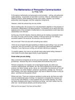
The n-Security Case
◆

For an n-security portfolio, the variance is:
n

n

σ = ∑∑ xi x j ρijσ iσ j
2
p

i =1 j =1

where xi = proportion of total investment in Security i

ρij = correlation coefficient between
Security i and Security j

18


The n-Security Case (cont’d)
◆

A covariance matrix is a tabular presentation of
the pairwise combinations of all portfolio

components
• The required number of covariances to compute
a portfolio variance is (n2 – n)/2
• Any portfolio construction technique using the
full covariance matrix is called a Markowitz
model
19


Example of Variance-Covariance
Matrix Computation in Excel

20


21


22


Portfolio Mathematics (Matrix Form)
◆
◆
◆
◆

Define w as the (vertical) vector of weights on the
different assets.
Define µ the (vertical) vector of expected returns

Let V be their variance-covariance matrix
The variance of the portfolio is thus:

σ = w 'Vw
2
p

Portfolio optimization consists of minimizing this
variance subject to the constraint of achieving a
given expected return.
23


Portfolio Variance in the 2-asset case
We have:
 wA 
w= 
 wB 

and

 σ A2 σ AB 
V =
2 
σ
σ
B 
 AB

Hence:

2

σ
σ AB   wA 
2
A
σ p = w 'Vw = [ wA wB ] 

2 
w
σ AB σ B   B 
σ p2 = wA2σ A2 + wB2σ B2 + 2wA wBσ AB

σ p2 = wA2σ A2 + wB2σ B2 + 2wA wB ρ ABσ Aσ B
24


Covariance Between Two Portfolios
(Matrix Form)
◆
◆
◆
◆
◆

Define w1 as the (vertical) vector of weights on
the different assets in portfolio P1.
Define w2 as the (vertical) vector of weights on
the different assets in portfolio P2.
Define µ the (vertical) vector of expected returns

Let V be their variance-covariance matrix
The covariance between the two portfolios is:

σ P1 , P2 = w1 'Vw2 = w2 'Vw1

(by symmetry)
25