Analysis and modelling of the hydraulic conductivity in aquitards application to the galilee basin and the great artesian basin, australia
Bạn đang xem bản rút gọn của tài liệu. Xem và tải ngay bản đầy đủ của tài liệu tại đây (5.92 MB, 165 trang )
Analysis and modelling of the hydraulic
conductivity in aquitards: application to the
Galilee Basin and the Great Artesian Basin,
Australia
Zhenjiao JIANG
Bachelor of Science (Jilin University, China), 2008
Master of Science (Jilin University, China), 2011
Thesis submitted in accordance with the regulations for
the Degree of Doctor of Philosophy
School of Earth, Environmental and Biological Sciences
Science and Engineering Faculty
Queensland University of Technology
2014
Key Words
Aquifer, aquitard, Bayesian inference, coal seam gas, coherence analysis,
cokriging interpolation, Eromanga Basin, fluvial processes, Galilee
Basin, geological process based model, Great Artesian Basin, harmonic
analysis, hydraulic conductivity, kriging interpolation, numerical
simulation,
perturbation
method,
accumulation, spectral analysis.
sediment
transport,
sediment
Abstract
The hydraulic conductivity (K) of an aquitard is of critical importance in controlling
groundwater flow and solute transport in a multilayered aquifer-aquitard system.
Direct measurement of K is commonly based on the Darcy’s law, which expresses a
linear relationship between K and pressure/water-level differences. As aquitards are
of low permeability, measurement of K in a realistic timeframe requires a large
pressure difference within the testing interval. As a consequence, direct K
measurement for an aquitard is mostly limited to the laboratory tests, where the
larger pressure difference can be controlled. But due to the scale effect induced by
the heterogeneity of the aquitard, the resultant K from laboratory tests can be several
orders different with K at the practical scale (such as the sizes of discretized cells in
the regional-scale numerical simulation for groundwater flow).
The focus of this dissertation is the development of alternative methods to enable
estimation of K in the aquitard at a regional scale, mainly including an analytical
approach and a geological process-based method.
The analytical approach, which combines the harmonic and coherence analysis,
is developed to calculate the vertical hydraulic conductivity (Kv) in the aquitard,
based on the long-term water-level measurements in the aquifers overlying and
underlying the target aquitard. The harmonic analysis derives Kv as a function of
leakage-induced water-level fluctuations in the aquifers. The coherence analysis
rules out the noise which interrupts the leakage-induced water-level fluctuations. The
method is validated by synthetic case studies, and then is applied to calculate Kv for
both the Westbourne and Birkhead aquitards within the Eromanga Basin, Australia.
From this, Kv for the Westbourne aquitard is estimated to be 2.17×10⁻⁵ m/d and for
the Birkhead aquitard is 4.31×10⁻⁵ m/d.
Combining harmonic and coherence analysis above can result in a regional-scale
Kv, which is, however, averaged over heterogeneity of the aquitard. As an alternative,
another methodology which can infer the heterogeneous K distribution in the
aquitard is proposed. The method is based on the fluvial processes simulation,
assuming that the target aquitard is formed by a river system. Steps in this
methodology are:
-1-
(1) 1D stochastic fluvial process-based model is developed on the basis of the
Exner equation, by revisiting the flow velocity in the model as the stochastic
description (mean and perturbation) of velocity. As a consequence, the riverbed and
channel evolution, and the variation of river discharge can be accounted in the
model. Two-phases of sediment transport (sand and silt) are modelled to reproduce a
sandstone/siltstone architecture (with respect to high/low permeable rock structure),
which result in 2D profiles of the sandstone proportion.
(2) The sill, nugget and correlation length of sandstone proportion is then
extracted, and is used in the kriging procedure to infer a 3D representation of
sandstone proportion.
(3) The sandstone proportion is converted to K values based on the classical
averaging method that vertical K is the harmonic average of original K in sandstone
and siltstone, whilst the horizontal K is the arithmetic average of K in sandstone and
siltstone.
The methodology is applied in the Betts Creek Beds (BCB), which is an aquitard
separating a key coalbed from several major aquifers in the Galilee Basin, Australia.
BCB was deposited by a river system in the Permian over a period of 20 million
years, and is composed by sandstone, siltstone, claystone and shale. K for the
siltstone, claystone and shale were tested by centrifuge permeameter core analysis. K
for sandstones are tested by the drill stem test, and also inferred from the downhole
logs of the electrical resistivity and sonic velocity using cokriging-Bayesian
approach. Herein, the fine-grained sediments (siltstone, claystone and shale) which
have similar K values are uniformly referred to as “siltstone”. The lithological
architecture (sandstone/siltstone) of BCB is simulated by combining the stochastic
fluvial process model and the kriging method. Finally, 3D spatial distribution of K
can be inferred by substituting K of sandstone and siltstone in the lithology
architecture. K measured by laboratory testing, field drill stem test and the cokriging
method represent the values on a small scale, but averaging methods, which convert
the lithological architecture to the heterogeneous K distribution, result in upscaled K
values.
-2-
Contents
Abstract………. .......................................................................................................... 1
Contents…… ............................................................................................................... 1
List of Figures ............................................................................................................... I
Acknowledgements .................................................................................................... III
Statement of Original Authorship ............................................................................... V
Statement of Contribution of Co-Authors ................................................................. VII
Thesis Outline .............................................................................................................. 1
Chapter 1: Introduction... ......................................................................................... 3
1.1 STUDY AREA ..............................................................................................................3
1.1.1 Regional geology ...................................................................................................3
1.1.2 Stratigraphy............................................................................................................5
1.1.3 Hydrogeological features .......................................................................................9
1.2 RESEARCH AIM ........................................................................................................10
Chapter 2: Methods review ..................................................................................... 13
2.1 ANALYTICAL METHOD..........................................................................................13
2.2 NUMERICAL INVERSION .......................................................................................14
2.3 GEOSTATISTICAL INTERPOLATION ...................................................................15
2.4 GEOLOGICAL PROCESS-BASED MODEL ............................................................17
2.5 HYBRID METHOD ....................................................................................................20
Chapter 3: Vertical hydraulic conductivity in the aquitards ............................... 21
Abstract ..............................................................................................................................21
Keywords ...........................................................................................................................21
3.0 INTRODUCTION .......................................................................................................21
3.1 METHODS ..................................................................................................................23
3.1.1 Harmonic analysis of water-level signals ............................................................23
3.1.2 Calculation of phases ...........................................................................................31
3.1.3 Selection of frequencies .......................................................................................32
3.1.4 Estimation of Kv ...................................................................................................33
3.1.5 Procedures ...........................................................................................................34
3.2 SYNTHETIC CASE STUDY ......................................................................................35
3.2.1 Influence of aquifer thickness on Kv estimation ..................................................36
3.2.2 Influence of observation-well distances ..............................................................38
3.2.3 Causal relationship...............................................................................................41
3.3 Hydraulic conductivity for the aquitards in the Great Artesian Basin .........................44
3.3.1 Materials ..............................................................................................................44
3.3.2 Estimates of hydraulic conductivity ....................................................................46
3.4 SUMMARY AND CONCLUSION ............................................................................49
Acknowledgements ............................................................................................................50
Chapter 4: Stochastic fluvial process model .......................................................... 51
Introductory comments ......................................................................................................51
Abstract ..............................................................................................................................51
-1-
Key words ......................................................................................................................... 52
4.0 INTRODUCTION ....................................................................................................... 53
4.1 GOVERNING EQUATION ....................................................................................... 55
4.2 VELOCITY REVISITED ........................................................................................... 56
4.2.1 Manning velocity ................................................................................................ 56
4.2.2 Velocity perturbation induced by turbulence ...................................................... 57
4.2.3 Define channel evolution in the ensemble statistics of velocity ......................... 57
4.3 MASS BALANCE EQUATION REVISITED ........................................................... 60
4.4 SEMI-ANALYTICAL SOLUTIONS ......................................................................... 63
4.4.1 Solution for the variance of sediment load.......................................................... 63
4.4.2 Solution for the mean sediment load ................................................................... 65
4.4.3 Solution for the mean and variance of sedimentation thickness ......................... 66
4.5 ALGORITHM ............................................................................................................. 67
4.6 SYNTHETIC CASES STUDY ................................................................................... 68
4.6.1 Synthetic example-1 ............................................................................................ 69
4.6.2 Synthetic example-2 ............................................................................................ 72
4.7 CONCLUSION ........................................................................................................... 73
Acknowledgment .............................................................................................................. 74
Chapter 5: Local-scale hydraulic conductivity determination ............................ 75
Introductory comment ....................................................................................................... 75
Abstract ............................................................................................................................. 75
Key Words ........................................................................................................................ 76
5.0 INTRODUCTION ....................................................................................................... 76
5.1 Study area and data description ................................................................................... 78
5.1.1 General geological setting ................................................................................... 78
5.1.2 Data analysis and pre-processing ........................................................................ 80
5.2 METHODOLOGY ...................................................................................................... 82
5.2.1 Bayesian framework............................................................................................ 82
5.2.2 Cokriging model ................................................................................................. 83
5.2.3 Normal linear regression model .......................................................................... 84
5.2.4 Theoretical differences between CK and NLR-based Bayesian method ............ 85
5.3 HYDRAULIC CONDUCTIVITY ESTIMATION ..................................................... 87
5.3.1 Prior estimation ................................................................................................... 87
5.3.2 Updating by Bayesian statistics .......................................................................... 88
5.3.3 Discussion ........................................................................................................... 91
5.4 CONCLUSION ........................................................................................................... 94
Acknowledgements ........................................................................................................... 94
Chapter 6: Heterogeneity of the Betts Creek Beds ............................................... 95
Introductory comment ....................................................................................................... 95
Abstract ............................................................................................................................. 95
Keyword ............................................................................................................................ 96
6.0 INTRODUCTION ....................................................................................................... 96
6.1 DEPOSITIONAL ENVIRONMENT OF BCB ........................................................... 99
6.2 METHOD.................................................................................................................. 100
6.2.1 Two facies sediment accumulation simulated by SFPM .................................. 101
6.2.2 Selection of kriging method .............................................................................. 101
6.3 WORKFLOW ........................................................................................................... 102
6.4 RESULTS AND DISCUSSIONS ............................................................................. 105
6.4.1 Sensitivity analysis ............................................................................................ 105
-2-
6.4.2 Model validation ................................................................................................106
6.4.3 3D heterogeneous hydraulic conductivity .........................................................111
6.4.4 Uncertainty ........................................................................................................113
6.5 SUMMARY ...............................................................................................................118
Acknowledgements ..........................................................................................................120
Chapter 7: Summary and conclusions ................................................................. 121
7.1 ANALYTICAL APPROACH ...................................................................................121
7.2 COKRIGING AND BAYES INTERPOLATION .....................................................122
7.3 STOCHASTIC FLUVIAL PROCESS-BASED APPROACH ..................................123
7.4 COMPARISION OF THREE METHODS ................................................................124
7.4.1 Analytical approach ...........................................................................................124
7.4.2 Coupled cokriging and Bayes method ...............................................................124
7.4.3 Process-based modelling ...................................................................................125
7.5 CONCLUSION ..........................................................................................................125
Appendix A: Drill Stem Test ................................................................................. 127
Appendix B: Centrifuge permeameter core analysis .......................................... 129
Appendix C: Erosion and deposition rate............................................................ 131
C.1 EROSION RATE ......................................................................................................131
C.2 DEPOSITION RATE ................................................................................................132
Appendix D: Conference abstracts ....................................................................... 133
Bibliography. .......................................................................................................... 135
-3-
List of Figures
Figure 1.1 Location map for the Galilee Basin. ........................................................ 4
Figure 1.2 Stratigraphic formations in the Galilee and Eromanga basins ................. 6
Figure 3.1 Schematic map of a three-layered leaky aquifer system........................ 24
Figure 3.2 Conceptualization of a synthetic example. ............................................ 35
Figure 3.3 Arbitrary water-level fluctuations and response. ................................... 36
Figure 3.4 Coherences between water-level signals. .............................................. 37
Figure 3.5 Estimates of C0 and Kv based on water-level fluctuations. .................... 38
Figure 3.6 Coherence between water-levels in lower and upper aquifer. ............... 39
Figure 3.7 Linear correlation between frequency and phase shift. ......................... 40
Figure 3.8 Estimates of Kv versus aquitard thickness and input signal. .................. 41
Figure 3.9 Impacts of energy effectiveness. ............................................................ 43
Figure 3.10 Multilayered leaky system that is being investigated. ......................... 45
Figure 3.11 Water-level measurements from 01/01/1919 to 2/10/1992. ................ 46
Figure 3.12 Frequencies versus higher coherence. ................................................. 47
Figure 3.13 Log-log relationship between frequency and phase shift. ................... 48
Figure 4.1 Simplification of braided and meandering rivers. ................................ 52
Figure 4.2 Probabilistic river channel occurrence and velocity perturbation. ....... 56
Figure 4.3 Flow chart of modelling sediment load and sedimentation thickness. .. 60
Figure 4.4 Sediment aggregation. ........................................................................... 70
Figure 4.5 Sediment degration. ............................................................................... 72
Figure 5.1 Location map of the northern Galilee Basin. ......................................... 79
Figure 5.2 Shales identified according to geophysical logs. ................................... 80
Figure 5.3 Histograms of sonic velocity and electrical resistivity.. ....................... 82
Figure 5.4 Linear relationships between electrical resistivity and permeability. .... 87
Figure 5.5 Estimates of permeability from cokriging Bayesian approaches........ ..89
Figure 5.6 Experimental and modelled covariance functions…….…………….…91
Figure 5.7 Scatterplots of permeability versus sonic velocity. ............................... 92
Figure 5.8 The permeability for the sandstones in the Betts Creek Beds. .............. 93
Figure 5.9 Hydraulic conductivity for the sandstones in the Betts Creek Beds. ..... 93
I
Figure 6.1 The target formation, Betts Creek Beds. ................................................ 97
Figure 6.2 Monthly sediment input in the Thompson River, Australia. ............... 103
Figure 6.3 Sensitivity analysis of sandstone proportion........................................ 106
Figure 6.4 Comparison of calculated and observed sandstone proportion............ 107
Figure 6.5 Relationship between observed and simulated thickness .................... 108
Figure 6.6 Observed and simulated sandstone proportion on 10 m interval. ........ 109
Figure 6.7 Sedimentation thickness and sandstone proportion in cross section. .. 110
Figure 6.8 Semivariogram of thickness and sandstone proportion. ...................... 112
Figure 6.9 3D heterogeneous pattern of hydraulic conductivity. .......................... 112
Figure 6.10 Five-layer conceptualized model and trigger stresses. ...................... 114
Figure 6.11 Influences of boundary condition and aquifer heterogeneity. ........... 114
Figure 6.12 Risk zone variation with simulation time. ......................................... 117
Figure 6.13 Uncertainty of hydraulic connectivity. .............................................. 118
Figure A1 General pressure variations within the Drill Stem Test process. ......... 127
Figure A2 Semi-log plot of pressure versus dimensionless time. ......................... 128
Figure B1 Hydraulic conductivity resulting from centrifuge permeameter. ......... 129
II
Acknowledgements
I have fortunately benefited from a good collaboration and environment with my
supervisors, and also postgraduate colleagues in QUT, as well as developing external
collaborations.
I greatly thank my principal supervisor, Prof. Malcolm Cox. He offered me an
opportunity to study in QUT three years ago. I also acknowledge my associate
supervisors: Dr. Mathias Raiber, Dr. Christoph Schrank, and Dr. Mauricio Taulis.
From them, I have learned how to do research, how to express my works in oral and
written forms.
I appreciate discussions with Dr. Gregoire Mariethoz from University of New
South Wales about geostatistics and fluvial process modeling, and thank his input in
my papers. I thank Prof. Chris Fielding in University of Nebraska-Lincoln for
suggestions on conceptualizing the deposition environment of Permian formations in
the Galilee Basin. These suggestions are essential to my work. I also thank Dr.
Wendy Timms and Dr. Dayna McGeeney from University of New South Wales for
their help with the operation of Centrifuge Permeameter.
I thank my office colleagues, Des Owen, Adam King, Clement Duvert, Martin
Labadz, Irina Romanova, Jorge Martinez, Stefan Groflin, Claudio Moya and Coralie
Siegel for their advices on my daily life and encouragements on my study. I spend a
very happy time with them.
I also thank QUT members Sarie Gould, Courtney Innes and Heather Campbell,
who always kindly answer my questions, and help me organise the trips and buy the
books.
My dissertation reading committee members are acknowledged.
I am grateful for funding from China Scholarship Council and Exoma Energy.
Special thanks are given to my parents, and my love Zha Enshuang. I can
understand what a difficult period it is when we were separated by Pacific Ocean and
can only communicate via the Skype. Thanks for your unwavering support.
III
Statement of Original Authorship
The work contained in this thesis has not been previously submitted to meet
requirements for an award at this or any other higher education institution. To the
best of my knowledge and belief, the thesis contains no material previously
published or written by another person except where due reference is made.
QUT Verified Signature
V
Statement of Contribution of Co-Authors
1. They meet the criteria for authorship in that they have participated in the
conception, execution, or interpretation, of at least that part of the publication in their
field of expertise;
2. They take public responsibility for their part of the publication, except for the
responsible author who accepts overall responsibility for the publications;
3. There are no other authors of the publication according to these criteria;
4. Potential conflicts of interest have been disclosed to (a) granting bodies, (b) the
editor or publisher of journals or other publications, and (c) the head of the
responsible academic unit, and
5. They agree to the use of publication in the student’s thesis and its publication on
the Australasian Digital Thesis database consistent with any limitations set by
publisher requirements.
Contributors
Zhenjiao Jiang, (Candidate)
Dr. Gregoire Mariethoz (Senior Lecturer in the University of New South Wales)
Dr. Matthias Raiber (Research Scientist in CSIRO)
Dr. Christoph Schrank (Lecturer in Queensland University of Technology)
Dr. Malcolm Cox (Professor in Queensland University of Technology)
Dr. Mauricio Taulis (Lecturer in Queensland University of Technology)
Dr. Wendy Timms (Lecturer in the University of New South Wales)
VII
Thesis Outline
This thesis is based on four publications, which are supported within the thesis by
background information and explanation. The study is largely of a “desktop” nature
with use of mathematical models, but utilises a wide range of available geological,
geophysical, drillhole and engineering data. The thesis content can be summarised as
follows:
Chapter 1: Introduction to the thesis aim and objectives, and an overview of
geology and hydrogeology of the study area.
Chapter 2: Reviews of the methods to infer hydraulic conductivity (K) in the
aquitard.
Chapter 3: Published Paper. Jiang, Z., Mariethoz, G., Taulis, M. and Cox, M.
(2013). Determination of vertical hydraulic conductivity of aquitards in a
multilayered leaky system using water-level signals in adjacent aquifers. Journal of
Hydrology, 500, pp. 170-182.
This paper describes a novel methodology to infer the regional-scale vertical
hydraulic conductivity in the aquitard based on water-level measurements in the
adjacent aquifers. The method is applied in the Great Artesian Basin, Australia.
Chapter 4: Submitted paper. Jiang, Z., Mariethoz, G., Schrank, C. and Cox, M. A
stochastic formulation of sediment accumulation and transport to characterize
alluvial formations (submitted to the Water Resources Research).
The manuscript derives a stochastic fluvial process model (SFPM), which can
simulate the sediment transport and accumulation, with regards to both the channel
and riverbed evolution, and can result in mean and variance of sedimentation
thickness.
Chapter 5: Published paper. Jiang, Z., Schrank, C., Mariethoz, G. and Cox, M.
(2013). Permeability estimation conditioned to geophysical downhole log data in
sandstones of the northern Galilee Basin, Queensland: methods and application.
Journal of Applied Geophysics, 93, pp. 43-51.
This paper develops a cokriging-Bayesian interpolation approach, which can
estimate the permeability of sandstones from the downhole geophysical logs of sonic
velocity and electrical resistivity. The resulting permeability can be converted to the
Thesis Outline
1
hydraulic conductivity, which is then used in the lithology architecture to infer the
3D K distribution (details in Chapter 6).
Chapter 6: Submitted paper. Jiang, Z., Raiber, M., Mariethoz, G., Timms, W. and
Cox, M. Three-dimensional hydraulic conductivity of the Betts Creek Beds in the
Northern Galilee Basin, Australia: insights from stochastic fluvial process modelling
and kriging interpolation (Submitted to the Journal of Hydrology).
This manuscript employs the SFPM derived in Chapter 4, with the assist of the
kriging approach, to construct the 3D heterogeneous hydraulic conductivity in the
Betts Creek Beds.
Chapter 7: Summary and conclusions for the findings of these individual papers and
the study overall.
Appendix: Supportive information such as drill stem test, centrifuge permeameter
test, expressions of deposition and erosion rate, and the abstracts of the oral
presentations in two international conferences.
Bibliography: All the references in the thesis, including those in the individual
manuscripts.
2
Thesis outline
1
Introduction
1.1 STUDY AREA
1.1.1 Regional geology
The Galilee Basin is a large intracratonic basin in central Queensland, Australia (Fig.
1.1a and 1.1b), which was formed during the Late Carboniferous to Triassic (Allen
and Fielding, 2007a; Allen and Fielding, 2007b). The basin is divided into northern
and southern parts by the Barcaldine Ridge, approximately at the latitude 24oS. The
northern Galilee Basin was developed in two regional depressions, the Koburra
Trough and Lovelle Depression, which are separated by the early Palaeozoic
Maneroo Platform (Fig. 1.1c) (Hawkins and Green, 1993a). The basin is largely
overlain by the Eromanga Basin, with a narrow outcrop zone in the eastern margin of
the basin. The focus of this current study is in developing methods to quantify the
hydraulic conductivity in the aquitard. The proposed methods are then implemented
in the eastern part of the north Galilee Basin and the overlying Eromanga Basin. The
area of this current study covers approximately 74 000 km2 (Fig. 1.1c).
The Galilee Basin developed by sequential crustal extension, passive thermal
subsidence, and then foreland crustal loading (Van Heeswijck, 2006; Allen and
Fielding, 2007a). Most of the basinal structures in the west of the study area manifest
northeasterly or northly trends, and were active during the basin development. The
structures continued to develop during the Late Triassic compression after the basin
formation (Hawkins, 1976; Van Heeswijck, 2006).
Sedimentary formations of the north Galilee Basin are commonly divided into
two major successions: the Joe Joe Group, and the Betts Creek Beds and related
formations. The Joe Joe Group deposited during the Late Carboniferous to Early
Permian forms the lower succession, which comprises, from old to young, the Lake
Galilee Sandstone, Jericho Formation, Edie Tuff Member, Jochmus Formation and
Aramac Coal Measures (Fig. 1.2). Tectonic uplift at the end of the Early Permian
resulted in the partial erosion of the Aramac Coal Measure, and formed an
unconformity upon which sediment of the second succession was deposited. The
second succession comprises the Betts Creek Beds (BCB), Rewan Formation,
Chapter 1: Introduction
3
Clematis Sandstone and Moolayember Formation (Evans, 1980; Allen and Fielding,
2007a).
In the Late Triassic, an east-west compressional episode resulted in uplifting,
folding and partial erosion of the Moolayember Formation prior to depositing the
sediments of the Eromanga Basin, from the early Jurassic until the Late Cretaceous.
The Eromanga Basin is composed of the Precipice Sandstone, Evergreen Formation,
Hutton Sandstone, Birkhead Formation, Adori Sandstone, Westbourne Formation
and Hooray Sandstone overlain by the Rolling Down Group. The Eromanga Basin is
a sub-basin of the Great Artesian Basin (Fig. 1.2) (Vincent et al., 1985).
Figure 1.1 (a) Location map for the Galilee Basin (After Jell, 2012), (b) the relationship of different
basins, (c) mapped structures and sites of the hydraulic conductivity measurements in the study area
(shaded).
4
Chapter 1: Introduction
1.1.2 Stratigraphy
The potential groundwater-bearing capacity within the stratigraphic formations
relates to the lithology composition and depositional environment, which are
summarized in Fig. 1.2 and described below.
Lake Galilee Sandstone (Late Carboniferous)
The Lake Galilee Sandstone is defined as the earliest unit of the Galilee Basin. It
consists of mainly fine to medium grained sandstone with minor mudstone, which
were deposited in the east part of the northern Galilee Basin by westerly flowing
braided rivers (Gray and Swarbrick, 1975).
Jericho Formation (Late Carboniferous)
The Jericho Formation overlies the Lake Galilee Sandstone in the Koburra
Trough. This unit is dominantly composed of mudstones and siltstones with
subordinate sandstones, with respect to the depositional environment dominated by
lacustrine with a fluvial interruption in a mild cool climate. In addition, the area also
experienced multi-phased glaciations between 317-308 Ma, lasting about 3 million
years (Jones and Fielding, 2004; Jones and Fielding, 2008).
Jochmus Formation (Early Permian)
The Jochmus Formation overlies the Jericho Formation, which were deposited in
the Koburra Trough by south-westerly flowing rivers, and were affected by the
glacial and volcanic activities. The formation is divided into lower and upper
intervals by the finer grained Edie Tuff Member, which is widely recognized in the
northern Galilee Basin. Both the lower and upper Jochmus Formation consist of fine
to coarse grained sandstones, with minor mudstones and siltstones. The lower
Jochmus Formation consists of coarser grain size than the upper interval (Hawkins
and Green, 1993a; Van Heeswijck, 2006).
Aramac Coal Measures (late Early Permian)
The Aramac Coal Measures is the uppermost unit of the Joe Joe Group. It is
composed of a lower sandstone unit with minor coal and mudstone, and an upper
coal unit which were deposited by widespread peat swamps (Henderson and
Stephenson, 1980).
Chapter 1: Introduction
5
Figure 1.2 The general stratigraphic formations in the Galilee and Eromanga basins, and their
lithological components. The number of hydraulic conductivity measured by drill stem test (DST) and
drill core analysis (Core test) is summarized. The major aquifers in the Great Artesian Basin are
marked in the last column.
Betts Creek Beds (Late Permian)
After a period of non-deposition, gentle uplifting and erosion, the Betts Creek
Beds were deposited upon the unconformity of the Aramac Coal Measures as
alluvial, coastal-plain settings (Allen and Fielding, 2007a). Two groups of facies
were identified within the formation as channel deposits and flood basin deposits.
6
Chapter 1: Introduction
The formation consists of conglomerate, interbedded sandstone and siltstone by the
deposition in the low-sinuosity rivers and debris flows, and sandy siltstone and
carbonaceous siltstone related to the deposition environments of proximal-distal
flood and lakes (Allen and Fielding, 2007a).
Rewan Formation (Early Triassic)
The Rewan Formation conformably overlies the Betts Creek Beds, and mainly
consists of the fine to coarse grained quartzose sandstone, siltstone and mudstone.
The sediment was supplied by westerly and southwesterly flowing rivers, and
occasionally by the intermittent lakes in a drier climate compared to the climate
during the Permian (Hawkins and Green, 1993a).
Clematis Sandstone (Early Triassic)
Clematis Sandstone overlies the Rewan Formation and is widely distributed in
the centre of the Koburra Trough. The unit consists mainly of fine to very coarse
sandstones, and subordinate siltstone and mudstone, which were deposited in braided
river systems (Hawkins and Green, 1993a).
Moolayember Formation (Middle Triassic)
The Moolayember Formation is the upmost unit in the Galilee Basin, and was
formed by low gradient, westerly flow rivers depositing large amount of silt and mud
into lakes, with minor coarse-grained sand (Hawkins and Green, 1993a). Much of the
Moolayember Formation was eroded, prior to the deposition of the Eromanga Basin
sequences.
Precipice Sandstone/Evergreen Formation (Middle Jurassic)
The Precipice Sandstone forms the lowermost unit of the Eromanga Basin and
overlies the unconformity of the Moolayember Formation. The upper Precipice
Sandstone and Evergreen Formation are time equivalents of the basal Jurassic unit in
the Surat Basin to the east (Fig. 1.1b). Sandstones of the Precipice Formation were
deposited by the medium energy braided stream, and the source of sands was from
the north and west of the Surat Basin (Jell, 2012).
The upward termination of the Precipice Sandstone deposition was followed by
the deposition of the Evergreen Formation comprised of mudstones, siltstones and
fine-grained sandstones. The abrupt sediment facies variation suggests the deposition
environments transforming from a medium energy fluvial regime to a near flatbottomed shallow lake. In addition, sediments of the Evergreen Formation are rich of
iron, which is regarded as the product of evaporation (Wiltshire, 1989).
Chapter 1: Introduction
7