Đề cương ôn lecture on algebra 1
Bạn đang xem bản rút gọn của tài liệu. Xem và tải ngay bản đầy đủ của tài liệu tại đây (844.93 KB, 119 trang )
Hanoi University of Science and Technology
Faculty of Applied mathematics and informatics
Advanced Training Program
Lecture on
Algebra
Assoc. Prof. Dr. Nguyen Thieu Huy
Hanoi 2008
Nguyen Thieu Huy, Lecture on Algebra
Preface
This Lecture on Algebra is written for students of Advanced Training Programs of
Mechatronics (from California State University –CSU Chico) and Material Science (from
University of Illinois- UIUC). When preparing the manuscript of this lecture, we have to
combine the two syllabuses of two courses on Algebra of the two programs (Math 031 of
CSU Chico and Math 225 of UIUC). There are some differences between the two syllabuses,
e.g., there is no module of algebraic structures and complex numbers in Math 225, and no
module of orthogonal projections and least square approximations in Math 031, etc.
Therefore, for sake of completeness, this lecture provides all the modules of knowledge
which are given in both syllabuses. Students will be introduced to the theory and applications
of matrices and systems of linear equations, vector spaces, linear transformations,
eigenvalue problems, Euclidean spaces,
orthogonal projections and least square
approximations, as they arise, for instance, from electrical networks, frameworks in
mechanics, processes in statistics and linear models, systems of linear differential equations
and so on. The lecture is organized in such a way that the students can comprehend the most
useful knowledge of linear algebra and its applications to engineering problems.
We would like to thank Prof. Tran Viet Dung for his careful reading of the manuscript. His
comments and remarks lead to better appearance of this lecture. We also thank Dr. Nguyen
Huu Tien, Dr. Tran Xuan Tiep and all the lecturers of Faculty of Applied Mathematics and
Informatics for their inspiration and support during the preparation of the lecture.
Hanoi, October 20, 2008
Assoc. Prof. Dr. Nguyen Thieu Huy
1
Nguyen Thieu Huy, Lecture on Algebra
Contents
Chapter 1: Sets.................................................................................. 4
I. Concepts and basic operations...........................................................................................4
II. Set equalities .................................................................................................................... 7
III. Cartesian products........................................................................................................... 8
Chapter 2: Mappings........................................................................ 9
I. Definition and examples....................................................................................................9
II. Compositions.................................................................................................................... 9
III. Images and inverse images ...........................................................................................10
IV. Injective, surjective, bijective, and inverse mappings .................................................. 11
Chapter 3: Algebraic Structures and Complex Numbers........... 13
I. Groups ............................................................................................................................. 13
II. Rings............................................................................................................................... 15
III. Fields............................................................................................................................. 16
IV. The field of complex numbers ......................................................................................16
Chapter 4: Matrices........................................................................ 26
I. Basic concepts ................................................................................................................. 26
II. Matrix addition, scalar multiplication ............................................................................28
III. Matrix multiplications...................................................................................................29
IV. Special matrices ............................................................................................................ 31
V. Systems of linear equations............................................................................................33
VI. Gauss elimination method ............................................................................................34
Chapter 5: Vector spaces ............................................................... 41
I. Basic concepts ................................................................................................................. 41
II. Subspaces ....................................................................................................................... 43
III. Linear combinations, linear spans.................................................................................44
IV. Linear dependence and independence ..........................................................................45
V. Bases and dimension......................................................................................................47
VI. Rank of matrices ...........................................................................................................50
VII. Fundamental theorem of systems of linear equations ................................................. 53
VIII. Inverse of a matrix .....................................................................................................55
X. Determinant and inverse of a matrix, Cramer’s rule......................................................60
XI. Coordinates in vector spaces ........................................................................................62
Chapter 6: Linear Mappings and Transformations .................... 65
I. Basic definitions .............................................................................................................. 65
II. Kernels and images ........................................................................................................67
III. Matrices and linear mappings .......................................................................................71
IV. Eigenvalues and eigenvectors....................................................................................... 74
V. Diagonalizations............................................................................................................. 78
VI. Linear operators (transformations) ............................................................................... 81
Chapter 7: Euclidean Spaces ......................................................... 86
I. Inner product spaces. .......................................................................................................86
II. Length (or Norm) of vectors ..........................................................................................88
III. Orthogonality ................................................................................................................ 89
IV. Projection and least square approximations: ................................................................94
V. Orthogonal matrices and orthogonal transformation .....................................................97
2
Nguyen Thieu Huy, Lecture on Algebra
IV. Quadratic forms ..........................................................................................................102
VII. Quadric lines and surfaces.........................................................................................108
3
Nguyen Thieu Huy, Lecture on Algebra
Chapter 1: Sets
I. Concepts and Basic Operations
1.1. Concepts of sets: A set is a collection of objects or things. The objects or things
in the set are called elements (or member) of the set.
Examples:
- A set of students in a class.
- A set of countries in ASEAN group, then Vietnam is in this set, but China is not.
- The set of real numbers, denoted by R.
1.2. Basic notations: Let E be a set. If x is an element of E, then we denote by x E
(pronounce: x belongs to E). If x is not an element of E, then we write x E.
We use the following notations:
: “there exists”
! : “there exists a unique”
: “ for each” or “for all”
: “implies”
: ”is equivalent to” or “if and only if”
1.3. Description of a set: Traditionally, we use upper case letters A, B, C and set
braces to denote a set. There are several ways to describe a set.
a) Roster notation (or listing notation): We list all the elements of a set in a couple
of braces; e.g., A = 1,2,3,7 or B = Vietnam, Thailand, Laos, Indonesia, Malaysia, Brunei,
Myanmar, Philippines, Cambodia, Singapore.
b) Set–builder notation: This is a notation which lists the rules that determine
whether an object is an element of the set.
Example: The set of real solutions of the inequality x2 2 is
G = x x R and -
2 x 2 = - 2, 2
The notation “” means “such that”.
4
Nguyen Thieu Huy, Lecture on Algebra
c) Venn diagram: Some times we use a closed figure on the plan to indicate a set.
This is called Venn diagram.
1.4 Subsets, empty set and two equal sets:
a) Subsets: The set A is called a subset of a set B if from x A it follows that x B.
We then denote by A B to indicate that A is a subset of B.
By logical expression: A B ( x A x B)
By Venn diagram:
A
B
b) Empty set: We accept that, there is a set that has no element, such a set is called
an empty set (or void set) denoted by .
Note: For every set A, we have that A.
c) Two equal sets: Let A, B be two set. We say that A equals B, denoted by A = B, if
A B and B A. This can be written in logical expression by
A = B (x A x B)
1.5. Intersection: Let A, B be two sets. Then the intersection of A and B, denoted by
A B, is given by:
A B = x xA and xB}.
This means that
x A B (x A and x B).
By Venn diagram:
1.6. Union: Let A, B be two sets, the union of A and B, denoted by AB, and given
by AB = {x xA or xB}. This means that
5
Nguyen Thieu Huy, Lecture on Algebra
x AB (x A or x B).
By Venn diagram:
1.7. Subtraction: Let A, B be two sets: The subtraction of A and B, denoted by A\B
(or A–B), is given by
A\B = {x | xA and xB}
This means that:
xA\B (x A and xB).
By Venn diagram:
1.8. Complement of a set:
Let A and X be two sets such that A X. The complement of A in X, denoted by
CXA (or A’ when X is clearly understood), is given by
CXA = X \ A = {x | xX
and x A)}
= {x | x A} (when X is clearly understood)
Examples: Consider X =R; A = [0,3] = {x | xR and 0 < x 3}
B = [-1, 2] = {x|xR and -1 x 2}.
Then,
1. AB = {xR | 0 x 3 and -1 x 2} =
= {x R | 0 x - 1} = [0, -1]
6
Nguyen Thieu Huy, Lecture on Algebra
2. AB = {xR | 0 x 3 or -1 x 2}
= {xR -1 x 3} = [-1,3]
3. A \ B = {x R 0 x 3 and x [-1,2]}
= {xR 2 x 3} = [2,3]
4. A’ = R \ A = {x R x < 0 or x > 3}
II. Set equalities
Let A, B, C be sets. The following set equalities are often used in many problems
related to set theory.
1. A B = BA; AB = BA
(Commutative law)
2. (AB) C = A(BC); (AB)C = A(BC) (Associative law)
3. A(BC) = (AB)(AC); A(BC) = (AB) (AC) (Distributive law)
4. A \ B = AB’, where B’=CXB with a set X containing both A and B.
Proof: Since the proofs of these equalities are relatively simple, we prove only one
equality (3), the other ones are left as exercises.
To prove (3), We use the logical expression of the equal sets.
x A
x A (B C)
x B C
x A
x B
x C
x A
xB
x A
x C
x A B
x A C
x(AB)(AC)
This equivalence yields that A(BC) = (AB)(AC).
The proofs of other equalities are left for the readers as exercises.
7
Nguyen Thieu Huy, Lecture on Algebra
III. Cartesian products
3.1. Definition:
1. Let A, B be two sets. The Cartesian product of A and B, denoted by AxB, is given
by
A x B = {(x,y)(xA) and (yB)}.
2. Let A1, A2…An be given sets. The Cartesian Product of A1, A2…An, denoted by
A1 x A2 x…x An, is given by A1 x A2 x….An = {(x1, x2…..xn)xi Ai = 1,2…., n}
In case, A1 = A2 = …= An = A, we denote
A1 x A2 x…x An = A x A x A x…x A = An.
3.2. Equality of elements in a Cartesian product:
1. Let A x B be the Cartesian Product of the given sets A and B. Then, two elements
(a, b) and (c, d) of A x B are equal if and only if a = c and b=d.
a c
In other words, (a, b) = (c, d)
b d
2. Let A1 x A2 x… xAn be the Cartesian product of given sets A1,…An.
Then, for (x1, x2…xn) and (y1, y2…yn) in A1 x A2 x….x An, we have that
(x1, x2,…, xn) = (y1, y2,…, yn) xi = yi i= 1, 2…., n.
8
Nguyen Thieu Huy, Lecture on Algebra
Chapter 2: Mappings
I. Definition and examples
1.1. Definition: Let X, Y be nonempty sets. A mapping with domain X and range Y,
is an ordered triple (X, Y, f) where f assigns to each xX a well-defined f(x) Y. The
f
statement that (X, Y, f) is a mapping is written by f: X Y (or X Y).
Here, “well-defined” means that for each xX there corresponds one and only one f(x) Y.
A mapping is sometimes called a map or a function.
1.2. Examples:
1. f: R R; f(x) = sinx xR, where R is the set of real numbers,
2. f: X X; f(x) = x x X. This is called the identity mapping on the set X,
denoted by IX
3. Let X, Y be nonvoid sets, and y0 Y. Then, the assignment f: X Y; f(x) = y0 x
X, is a mapping. This is called a constant mapping.
1.3. Remark: We use the notation
f: X Y
x f(x)
to indicate that f(x) is assigned to x.
f
1.4. Remark: Two mapping X Y and
g
X Y are equal if f(x) = g(x) x X.
Then, we write f=g.
II. Compositions
2.1. Definition: Given two mappings: f: X Y and g: Y W (or shortly,
g
f
X Y W), we define the mapping h: X W by h(x) = g(f(x)) x X. The mapping h
is called the composition of g and f, denoted by h = gof, that is, (gof)(x) = g(f(x)) xX.
g
f
2.2. Example: R R+ R-, here R+=[0, ] and R-=(-, 0].
f(x) = x2 xR; and g(x) = -x x R+. Then, (gof)(x) = g(f(x)) = -x2.
2.3. Remark: In general, fog gof.
g
f
Example: R R R; f(x) = x2; g(x) = 2x + 1 x R.
9
Nguyen Thieu Huy, Lecture on Algebra
Then (fog)(x) = f(g(x)) = (2x+1)2 x R, and (gof)(x) = g(f(x)) = 2x2 + 1 x R
Clearly, fog gof.
III. Image and Inverse Images
Suppose that f: X Y is a mapping.
3.1. Definition: For S X, the image of S in a subset of Y, which is defined by
f(S) = {f(s)sS} = {yYsS with f(s) = y}
Example: f: R R, f(x) = x2+2x x R.
S = [0,2] R; f(S) = {f(s)s[0, 2]} = {s2s[0, 2]} = [0, 8].
3.2. Definition: Let T Y. Then, the inverse image of T is a subset of X, which is
defined by f-1(T) = {xXf(x) T}.
Example: f: R\ {2} R; f(x) =
x 1
xR\{2}.
x2
S = (-, 1] R; f-1(S) = {xR\{2}f(x) -1}
= {xR\{2}
x 1
- 1 }= [-1/2,2).
x2
3.3. Definition: Let f: X Y be a mapping. The image of the domain X, f(X), is
called the image of f, denoted by Imf. That is to say,
Imf = f(X) = {f(x)xX} = {y YxX with f(x) = y}.
3.4. Properties of images and inverse images: Let f: X Y be a mapping; let A, B
be subsets of X and C, D be subsets of Y. Then, the following properties hold.
1) f(AB) = f(A) f(B)
2) f(AB) f(A) f(B)
3) f-1(CD) = f-1(C) f-1(D)
4) f-1(CD) = f-1(C) f-1(D)
Proof: We shall prove (1) and (3), the other properties are left as exercises.
(1) : Since A A B and B AB, it follows that
f(A) f(AB) and f(B) f(AB).
10
Nguyen Thieu Huy, Lecture on Algebra
These inclusions yield f(A) f(B) f(AB).
Conversely, take any y f(AB). Then, by definition of an Image, we have that, there exists
an x A B, such that y = f(x). But, this implies that y = f(x) f(A) (if x A) or y=f(x)
f(B) (if x B). Hence, y f(A) f(B). This yields that f(AB) f(A) f(B). Therefore,
f(AB) = f(A) f(B).
(3): xf-1(CD) f(x) CD (f(x) C or f(x) D)
(x f-1(C) or x f-1(D)) x f-1(C)f-1(D)
Hence, f-1(CD) = f-1(D)) = f-1(C)f-1(D).
IV. Injective, Surjective, Bijective, and Inverse Mappings
4.1. Definition: Let f: X Y be a mapping.
a. The mapping is called surjective (or onto) if Imf = Y, or equivalently,
yY, xX such that f(x) = y.
b. The mapping is called injective (or one–to–one) if the following condition holds:
For x1,x2X if f(x1) = f(x2), then x1 = x2.
This condition is equivalent to:
For x1,x2X if x1x2, then f(x1) f(x2).
c. The mapping is called bijective if it is surjective and injective.
Examples:
f
1. R R; f(x) = sinx x R.
This mapping is not injective since f(0) = f(2) = 0. It is also not surjective, because,
f(R) = Imf = [-1, 1] R
2. f: R [-1,1], f(x) = sinx xR. This mapping is surjective but not injective.
3. f: , R; f(x) = sinx x , . This mapping is injective but not
2 2
2 2
surjective.
, [-1,1]; f(x) = sinxx , . This mapping is bijective.
2 2
2 2
4. f :
11
Nguyen Thieu Huy, Lecture on Algebra
4.2. Definition: Let f: X Y be a bijective mapping. Then, the mapping g: Y X
satisfying gof = IX and fog = IY is called the inverse mapping of f, denoted by g = f-1.
For a bijective mapping f: X Y we now show that there is a unique mapping g: Y X
satisfying gof = IX and fog = IY.
In fact, since f is bijective we can define an assignment g : Y X by g(y) = x if f(x) = y.
This gives us a mapping. Clearly, g(f(x)) = x x X and f(g(y)) = y yY. Therefore,
gof=IX and fog = IY.
The above g is unique is the sense that, if h: Y X is another mapping satisfying hof
= IX and foh = IY, then h(f(x)) = x = g(f(x)) x X. Then, y Y, by the bijectiveness of f,
! x X such that f(x) = y h(y) = h(f(x)) = g(f(x)) = g(y). This means that h = g.
Examples:
, 1,1; f(x) = sinx x
2 2
1. f:
2 , 2
This mapping is bijective. The inverse mapping f-1 : 1,1 ; , is denoted by
2 2
f-1 = arcsin, that is to say, f-1(x) = arcsinx x [-1,1]. We also can write:
, ; and sin(arcsinx)=x x [-1,1]
2 2
arcsin(sinx)=x x
2. f: R (0,); f(x) = ex x R.
The inverse mapping is f-1: (0, ) R, f-1(x) = lnx x (0,). To see this, take (fof-1)(x) =
elnx = x x (0,); and (f-1of)(x) = lnex = x x R.
12
Nguyen Thieu Huy, Lecture on Algebra
Chapter 3: Algebraic Structures and Complex Numbers
I. Groups
1.1. Definition: Suppose that G is non empty set and : GxG G is a mapping.
Then, is called a binary operation; and we will write (a,b) = ab for each (a,b) GxG.
Examples:
1) Consider G = R; “” = “+” (the usual addition in R) is a binary operation defined
by
+:
RxRR
(a,b) a + b
2) Take G = R; “” = “” (the usual multiplication in R) is a binary operation defined
by
:
RxRR
(a,b) a b
3. Take G = {f: X X f is a mapping}:= Hom (X) for X .
The composition operation “o” is a binary operation defined by:
o:
Hom(X) x Hom(X) Hom(X)
(f,g) fog
1.2. Definition:
a. A couple (G, ), where G is a nonempty set and is a binary operation, is called an
algebraic structure.
b. Consider the algebraic structure (G, ) we will say that
(b1) is associative if (ab) c = a(bc) a, b, and c in G
(b2) is commutative if ab = ba a, b G
(b3) an element e G is the neutral element of G if
ea = ae = a aG
13
Nguyen Thieu Huy, Lecture on Algebra
Examples:
1. Consider (R,+), then “+” is associative and commutative; and 0 is a neutral
element.
2. Consider (R, ), then “” is associative and commutative and 1 is an neutral
element.
3. Consider (Hom(X), o), then “o” is associative but not commutative; and the
identity mapping IX is an neutral element.
1.3. Remark: If a binary operation is written as +, then the neutral element will be
denoted by 0G (or 0 if G is clearly understood) and called the null element.
If a binary operation is written as , then the neutral element will be denoted by 1G
(or 1) and called the identity element.
1.4. Lemma: Consider an algebraic structure (G, ). Then, if there is a neutral
element e G, this neutral element is unique.
Proof: Let e’ be another neutral element. Then, e = ee’ because e’ is a neutral
element and e’ = ee’ because e is a neutral element of G. Therefore e = e’.
1.5. Definition: The algebraic structure (G, ) is called a group if the following
conditions are satisfied:
1. is associative
2. There is a neutral element eG
3. a G, a’ G such that aa’ = a’a = e
Remark: Consider a group (G, ).
a. If is written as +, then (G,+) is called an additive group.
b. If is written as , then (G, ) is called a multiplicative group.
c. If is commutative, then (G, ) is called abelian group (or commutative group).
d. For a G, the element a’G such that aa’ = a’a=e, will be called the opposition
of a, denoted by
a’ = a-1, called inverse of a, if is written as (multiplicative group)
a’ = - a, called negative of a, if is written as + (additive group)
14
Nguyen Thieu Huy, Lecture on Algebra
Examples:
1. (R, +) is abelian additive group.
2. (R\{0}, ) is abel multiplicative group.
3. Let X be nonempty set; End(X) = {f: X X f is bijective}.
Then, (End(X), o) is noncommutative group with the neutral element is IX, where o is
the composition operation.
1.6. Proposition:
Let (G, ) be a group. Then, the following assertions hold.
1. For a G, the inverse a-1 of a is unique.
2. For a, b, c G we have that
ac = bc a = b
ca = cb a = b
(Cancellation law in Group)
3. For a, x, b G, the equation ax = b has a unique solution x = a-1b.
Also, the equation xa = b has a unique solution x = ba-1
Proof:
1. Let a’ be another inverse of a. Then, a’a = e. It follows that
(a’a) a-1 = a’ (aa-1) = a’e = a’.
2. ac = ab a-1 (ac) a-1 (ab) (a-1a) c = (a-1a) b ec = eb c = b.
Similarly, ca = ba c = b.
The proof of (3) is left as an exercise.
II. Rings
2.1. Definition: Consider triple (V, +, ) where V is a nonempty set; + and
are
binary operations on V. The triple (V, +, ) is called a ring if the following properties are
satisfied:
15
Nguyen Thieu Huy, Lecture on Algebra
(V, +) is a commutative group
Operation “” is associative
a,b,c V we have that (a + b) c = ac + bc, and c(a + b) = ca + cb
V has identity element 1V corresponding to operation “” , and we call 1V the
multiplication identity.
If, in addition, the multiplicative operation is commutative then the ring (V, +, ) is called a
commutative ring.
2.2. Example: (R, +, ) with the usual additive and multiplicative operations, is a
commutative ring.
2.3. Definition: We say that the ring is trivial if it contains only one element, V =
{OV}.
Remark: If V is a nontrivial ring, then 1V OV.
2.4. Proposition: Let (V, +, ) be a ring. Then, the following equalities hold.
1. a.OV = OV.a = OV
2. a (b – c) = ab – ac, where b – c is denoted for b + (-c)
3. (b–c) a = ba – ca
III. Fields
3.1. Definition: A triple (V, +, ) is called a field if (V, +, ) is a commutative,
nontrivial ring such that, if a V and a OV then a has a multiplicative inverse a-1 V.
Detailedly, (V, +, ) is a field if and only if the following conditions hold:
(V, +) is a commutative group,
the multiplicative operation is associative and commutative,
a,b,cV we have that (a + b) c = ac + ab,
there is multiplicative identity 1V OV; and if aV, a OV, then a-1 V, a-1a = 1V.
3.2. Examples: (R, +, ); (Q, +, ) are fields.
IV. The field of complex numbers
Equations without real solutions, such as x2 + 1 = 0 or x2 – 10x + 40 = 0, were
observed early in history and led to the introduction of complex numbers.
16
Nguyen Thieu Huy, Lecture on Algebra
4.1. Construction of the field of complex numbers: On the set R2, we consider
additive and multiplicative operations defined by
(a,b) + (c,d) = (a + c, b + d)
(a,b) (c,d) = (ac - bd, ad + bc)
Then, (R2, +, ) is a field. Indeed,
1) (R2, +, ) is obviously a commutative, nontrivial ring with null element (0, 0) and
identity element (1,0) (0,0).
2) Let now (a,b) (0,0), we see that the inverse of (a,b) is (c,d) =
b
b
a
a
, 2
, 2
since (a,b)
2
= (1,0).
2
2
2
2
a b
a b2
a b
a b
We can present R2 in the plane
We remark that if two elements (a,0), (c,0) belong to horizontal axis, then their sum
(a,0) + (c,0) = (a + c, 0) and their product (a,0)(c,0) = (ac, 0) are still belong to the
horizontal axis, and the addition and multiplication are operated as the addition and
multiplication in the set of real numbers. This allows to identify each element on the
horizontal axis with a real number, that is (a,0) = a R.
Now, consider i = (0,1). Then, i2 = i.i = (0, 1). (0, 1) = (-1, 0) = -1. With this notation,
we can write: for (a,b) R2
(a,b) = (a,0) (1,0) + (b,0) (0,1) = a + bi
17
Nguyen Thieu Huy, Lecture on Algebra
We set C = {a + bia,b R and i2 = -1} and call C the set of complex numbers. It follows
from above construction that (C, +, ) is a field which is called the field of complex
numbers.
The additive and multiplicative operations on C can be reformulated as.
(a+bi) + (c+di) = (a+c) + (b+d)i
(a+bi) (c+di) = ac + bdi2 + (ad + bc)i = (ac – bd) + (ad + bc)i
(Because i2=-1).
Therefore, the calculation is done by usual ways as in R with the attention that i2 = -1.
The representation of a complex number z C as z = a + bi for a,bR and i2 = -1, is called
the canonical form (algebraic form) of a complex number z.
4.2. Imaginary and real parts: Consider the field of complex numbers C. For z C,
in canonical form, z can be written as
z = a + bi, where a, b R and i2 = -1.
In this form, the real number a is called the real part of z; and the real number b is called the
imaginary part. We denote by a = Rez and b = Imz. Also, in this form, two complex numbers
z1 = a1 + b1i and z2 = a2 + b2i are equal if and only if a1 = a2; b1 = b2, that is, Rez1=Rez2 and Imz1 = Imz2.
4.3. Subtraction and division in canonical forms:
1) Subtraction: For z1 = a1 + b1i and z2 = a2 + b2i, we have
z1 – z2 = a1 – a2 + (b1 – b2)i.
Example: 2 + 4i – (3 + 2i) = -1 + 2i.
2) Division: By definition,
z1
z1 ( z 21 )
z2
For z2 = a2 + b2i, we have z 21
a
a1 b1i
bi
a1 b1i . 2 2 2 2 2 2
a 2 b2
a 2 b2 a 2 b2
practical rule: To compute
(z2 0).
a2
b
2 2 2 i . Therefore,
2
a b2 a 2 b2
2
2
. We also have the following
z1 a1 b1i
we multiply both denominator and numerator by
z 2 a 2 b2 i
a2 – b2i, then simplify the result. Hence,
18
Nguyen Thieu Huy, Lecture on Algebra
a1 b1i a1 b1i a2 b2i a1a2 b1b2 a2b1 a1b2 i
.
a2 b2i a2 b2i a2 b2i
a22 b22
Example:
2 7i 2 7i 8 3i 5 62i 5 62
.
i
8 3i 8 3i 8 3i
73
73 73
4.4. Complex plane: Complex numbers admit two natural geometric interpretations.
First, we may identify the complex number x + yi with the point (x,y) in the plane
(see Fig.4.2). In this interpretation, each real number a, or x+ 0.i, is identified with the point
(x,0) on the horizontal axis, which is therefore called the real axis. A number 0 + yi, or just
yi, is called a pure imaginary number and is associated with the point (0,y) on the vertical
axis. This axis is called the imaginary axis. Because of this correspondence between complex
numbers and points in the plane, we often refer to the xy-plane as the complex plane.
Figure 4.2
When complex numbers were first noticed (in solving polynomial equations),
mathematicians were suspicious of them, and even the great eighteen–century Swiss
mathematician Leonhard Euler, who used them in calculations with unparalleled proficiency,
did not recognize then as “legitimate” numbers. It was the nineteenth–century German
mathematician Carl Friedrich Gauss who fully appreciated their geometric significance and
used his standing in the scientific community to promote their legitimacy to other
mathematicians and natural philosophers.
The second geometric interpretation of complex numbers is in terms of vectors. The
complex numbers z = x + yi may be thought of as the vector x i +y j in the plane, which may
in turn be represented as an arrow from the origin to the point (x,y), as in Fig.4.3.
19
Nguyen Thieu Huy, Lecture on Algebra
z
Fig. 4.3. Complex numbers as vectors in the plane
Fig.4.4. Parallelogram law for addition of complex numbers
The first component of this vector is Rez, and the second component is Imz. In this
interpretation, the definition of addition of complex numbers is equivalent to the
parallelogram law for vector addition, since we add two vectors by adding the respective
component (see Fig.4.4).
4.5. Complex conjugate: Let z = x +iy be a complex number then the complex
conjugate z of z is defined by z = x – iy.
It follows immediately from definition that
Rez = x = (z + z )/2; and Imz = y = (z - z )/2
We list here some properties related to conjugation, which are easy to prove.
1. z1 z 2 z1 z 2
2. z1 .z 2 z1 .z 2
z1, z2 in C
z1, z2 in C
20
Nguyen Thieu Huy, Lecture on Algebra
z
3. 1
z2
z1
z2
z1, z2 in C
4. if α R and z C, then .z .z
5. For z C we have that, z R if and only if z z .
4.6. Modulus of complex numbers: For z = x + iy C we define z= x y ,
2
2
and call it modulus of z. So, the modulus z is precisely the length of the vector which
represents z in the complex plane.
z = x + i.y = OM
z= OM = x y
2
2
4.7. Polar (trigonometric) forms of complex numbers:
The canonical forms of complex numbers are easily used to add, subtract, multiply or
divide complex numbers. To do more complicated operations on complex numbers such as
taking to the powers or roots, we need the following form of complex numbers.
Let we start by employ the polar coordination: For z = x + iy
x r cos
0 z = x + iy = OM = (x,y). Then we can put
y r sin
where
r = z =
x2 y2
(I)
and is angle between OM and the real axis, that is, the angle is defined by
x
cos
2
x y2
y
sin
x2 y2
(II)
The equalities (I) and (II) define the unique couple (r, ) with 0<2 such that
x r cos
. From this representation we have that
y r sin
21
Nguyen Thieu Huy, Lecture on Algebra
z = x + iy =
x2 y2
x
x2 y2
i
2
2
x y
y
= z(cos + isin).
Putting z = r we obtain
z = r(cos+isin).
This form of a complex number z is called polar (or trigonometric) form of complex
numbers, where r = z is the modulus of z; and the angle is called the argument of z,
denoted by = arg (z).
Examples:
1) z = 1 + i =
1
1
2
i
2 cos i sin
4
4
2
2
1
3
6 cos i sin
i
2 2
3
3
2) z = 3 - 3 3i 6
Remark: Two complex number in polar forms z1 = r1(cos1 + isin1); z2 = r2(cos2 +
isin2) are equal if and only if
r1 r2
1 2 2 k
k Z.
4.8. Multiplication, division in polar forms:
We now consider the multiplication and division of complex numbers represented in polar
forms.
1) Multiplication: Let z1 = r1(cos1 + isin1) ; z2 = r2(cos2+isin2)
Then, z1.z2 = r1r2[cos1cos2 - sin1sin2+i(cos1sin2 + cos2sin1)]. Therefore,
z1.z2 = r1r2[cos(1+2) + isin(1+2)].
It follows that z1.z2=z1.z2 and arg (z1.z2) = arg(z1) + arg(z2).
2) Division: Take z =
z1
z1 z.z 2 z1 = z.z2 (for z2 0)
z2
22
(4.1)
Nguyen Thieu Huy, Lecture on Algebra
z1
z =
z2
Moreover, arg(z1) = argz+argz2 arg(z) =arg(z1) – arg(z2).
Therefore, we obtain that, for z1=r1(cos1+isin1) and z2 = r2(cos2 + isin2) 0.
z1
r
z 1 [cos(1-2) + isin(1-2)].
z2
r2
We have that
(4.2)
z1 = -2 + 2i; z2 = 3i.
Example:
3
5
i sin
We first write z1 = 2 2 cos
; z 2 3 cos i sin
4
5
2
2
Therefore,
5
5
i sin
z1.z2 = 6 2 cos
4
4
z1 2 2
5
cos i sin
z2
4
3
4
3) Integer power: for z = r(cos + isin), by equation (4.1), we see that
z2 = r2(cos2 + isin2).
By induction, we easily obtain that zn = rn(cosn + isinn) for all nN.
Now, take z-1 =
1 1
cos( ) i sin( ) r 1 cos( ) i sin( ) .
z r
Therefore z-2 = z 1
2
r 2 cos(2 ) i sin(2 ) .
Again, by induction, we obtain: z-n = r-n(cos(-n) + isin(-n)) nN.
This yields that zn = rn(cosn + isinn) for all n Z.
A special case of this formula is the formula of de Moivre:
(cos + isin)n = cosn + isinn
nN.
Which is useful for expressing cosn and sinn in terms of cos and sin.
4.9. Roots: Given z C, and n N* = N \ {0}, we want to find all w C such that wn = z.
To find such w, we use the polar forms. First, we write z = r(cos + isin) and w = (cos +
isin). We now determine and . Using relation wn = z, we obtain that
23
Nguyen Thieu Huy, Lecture on Algebra
n(cosn + isinn) = r(cos + isin)
n r (real positive root of r)
n r
2k
;k Z
n 2k ; k Z
n
Note that there are only n distinct values of w, corresponding to k = 0, 1…, n-1. Therefore, w
is one of the following values
n
2 k
2 k
i sin
k 0,1..., n 1
r cos
n
n
For z = r(cos + isin) we denote by
n
and call
n
z n
2k
2k
r cos
i sin
k 0,1,2...n 1
n
n
z the set of all nth roots of complex number z.
For each w C such that wn = z, we call w an nth root of z and write w
n
z.
Examples:
1. 3 1 3 1(cos 0 i sin 0) (complex roots)
2k
2k
= 1 cos
i sin
k 0,1,2
3
3
= 1;
1
3 1
3
i;
i
2 2
2 2
2. Square roots: For Z = r(cos+isin) C, we compute the complex square roots
z r cos i sin =
2k
2k
= r cos
i sin
k 0,1
2
2
= r cos i sin ; r cos i sin . Therefore, for z 0; the set
2
2
2
2
contains two opposite values {w, -w}. Shortly, we write
Also, we have the practical formula, for z = x + iy,
24
z w (for w2 = z).
z