Chapter 9 net present value and other investment criteria

264

PA RT 4

Capital Budgeting

PA RT 4

9

Capital Budgeting

NET PRESENT VALUE AND
OTHER INVESTMENT CRITERIA

By 2006, the manufacture of large jet airplanes had

Boeing’s development of the Dreamliner offers an

shrunk to two major competitors, Boeing and Airbus.

example of a capital budgeting decision. A product

The competition between the two was stiff. In an

introduction such as this one, with a price tag in the

effort to increase its market share, Boeing began

billions, is obviously a major undertaking, and the

development of the 787 Dreamliner.

risks and rewards must be carefully weighed. In this

Designed to carry 200 to 300 passengers, the
Dreamliner was a

chapter, we discuss the basic tools used in making
such decisions.

Visit us at www.mhhe.com/rwj

radical departure

DIGITAL STUDY TOOLS

from previous

capital budgeting. Back in Chapter 1, we saw that

• Self-Study Software
• Multiple-Choice Quizzes
• Flashcards for Testing and
Key Terms

airplanes. The

increasing the value of the stock in a company is the

lightweight, one-

goal of financial management. Thus, what we need

piece, carbon

to learn is how to tell whether a particular investment

fiber fuselage

will achieve that. This chapter considers a variety of

replaced about

techniques that are actually used in practice. More

This chapter introduces you to the practice of

1,200 sheets of aluminum and 40,000 rivets, reducing

important, it shows how many of these techniques

weight by 15 percent. Additionally, the new engines

can be misleading, and it explains why the net present

had larger fans that were expected to reduce fuel con-

value approach is the right one.

sumption by 20 percent. The estimated development

cost of the Dreamliner? Over $8 billion!

In Chapter 1, we identified the three key areas of concern to the financial manager. The
first of these involved the question: What fixed assets should we buy? We called this
the capital budgeting decision. In this chapter, we begin to deal with the issues that arise
in answering this question.
The process of allocating or budgeting capital is usually more involved than just deciding whether to buy a particular fixed asset. We frequently face broader issues like whether
we should launch a new product or enter a new market. Decisions such as these determine
the nature of a firm’s operations and products for years to come, primarily because fixed
asset investments are generally long-lived and not easily reversed once they are made.
The most fundamental decision a business must make concerns its product line. What services will we offer or what will we sell? In what markets will we compete? What new products
will we introduce? The answer to any of these questions will require that the firm commit its
scarce and valuable capital to certain types of assets. As a result, all of these strategic issues fall
under the general heading of capital budgeting. The process of capital budgeting could thus be
given a more descriptive (not to mention impressive) name: strategic asset allocation.
264

ros3062x_Ch09.indd 264

2/23/07 9:32:35 PM


CHAPTER 9

265

Net Present Value and Other Investment Criteria

For the reasons we have discussed, the capital budgeting question is probably the most
important issue in corporate finance. How a firm chooses to finance its operations (the

capital structure question) and how a firm manages its short-term operating activities
(the working capital question) are certainly issues of concern, but the fixed assets define
the business of the firm. Airlines, for example, are airlines because they operate airplanes,
regardless of how they finance them.
Any firm possesses a huge number of possible investments. Each possible investment is
an option available to the firm. Some options are valuable and some are not. The essence of
successful financial management, of course, is learning to identify which are which. With
this in mind, our goal in this chapter is to introduce you to the techniques used to analyze
potential business ventures to decide which are worth undertaking.
We present and compare a number of different procedures used in practice. Our primary
goal is to acquaint you with the advantages and disadvantages of the various approaches.
As we will see, the most important concept in this area is the idea of net present value. We
consider this next.

Net Present Value

9.1

In Chapter 1, we argued that the goal of financial management is to create value for the
stockholders. The financial manager must thus examine a potential investment in light of
its likely effect on the price of the firm’s shares. In this section, we describe a widely used
procedure for doing this: The net present value approach.

THE BASIC IDEA
An investment is worth undertaking if it creates value for its owners. In the most general
sense, we create value by identifying an investment worth more in the marketplace than
it costs us to acquire. How can something be worth more than it costs? It’s a case of the
whole being worth more than the cost of the parts.
For example, suppose you buy a run-down house for $25,000 and spend another $25,000
on painters, plumbers, and so on to get it fixed up. Your total investment is $50,000. When

the work is completed, you place the house back on the market and find that it’s worth
$60,000. The market value ($60,000) exceeds the cost ($50,000) by $10,000. What you
have done here is to act as a manager and bring together some fixed assets (a house), some
labor (plumbers, carpenters, and others), and some materials (carpeting, paint, and so on).
The net result is that you have created $10,000 in value. Put another way, this $10,000 is
the value added by management.
With our house example, it turned out after the fact that $10,000 in value had been
created. Things thus worked out nicely. The real challenge, of course, would have been to
somehow identify ahead of time whether investing the necessary $50,000 was a good idea
in the first place. This is what capital budgeting is all about—namely, trying to determine
whether a proposed investment or project will be worth more, once it is in place, than it
costs.
For reasons that will be obvious in a moment, the difference between an investment’s
market value and its cost is called the net present value of the investment, abbreviated
NPV. In other words, net present value is a measure of how much value is created or added
today by undertaking an investment. Given our goal of creating value for the stockholders,
the capital budgeting process can be viewed as a search for investments with positive net
present values.

ros3062x_Ch09.indd 265

2/9/07 11:19:49 AM


266

PA RT 4

net present value
(NPV)

With our run-down house, you can probably imagine how we would go about making
the capital budgeting decision. We would first look at what comparable, fixed-up properties
were selling for in the market. We would then get estimates of the cost of buying a particular
property and bringing it to market. At this point, we would have an estimated total cost and an
estimated market value. If the difference was positive, then this investment would be worth
undertaking because it would have a positive estimated net present value. There is risk, of
course, because there is no guarantee that our estimates will turn out to be correct.
As our example illustrates, investment decisions are greatly simplified when there is a
market for assets similar to the investment we are considering. Capital budgeting becomes
much more difficult when we cannot observe the market price for at least roughly comparable investments. The reason is that we then face the problem of estimating the value of
an investment using only indirect market information. Unfortunately, this is precisely the
situation the financial manager usually encounters. We examine this issue next.

The difference between an
investment’s market value
and its cost.

Capital Budgeting

ESTIMATING NET PRESENT VALUE

discounted cash flow
(DCF) valuation
The process of valuing an
investment by discounting
its future cash flows.

Find out more
about capital budgeting for

small businesses at www.
smallbusinesslearning.net.

Imagine we are thinking of starting a business to produce and sell a new product—say organic
fertilizer. We can estimate the start-up costs with reasonable accuracy because we know
what we will need to buy to begin production. Would this be a good investment? Based on
our discussion, you know that the answer depends on whether the value of the new business
exceeds the cost of starting it. In other words, does this investment have a positive NPV?
This problem is much more difficult than our “fixer upper” house example because
entire fertilizer companies are not routinely bought and sold in the marketplace, so it is
essentially impossible to observe the market value of a similar investment. As a result, we
must somehow estimate this value by other means.
Based on our work in Chapters 5 and 6, you may be able to guess how we will go about
estimating the value of our fertilizer business. We will first try to estimate the future cash
flows we expect the new business to produce. We will then apply our basic discounted cash
flow procedure to estimate the present value of those cash flows. Once we have this estimate, we will then estimate NPV as the difference between the present value of the future
cash flows and the cost of the investment. As we mentioned in Chapter 5, this procedure is
often called discounted cash flow (DCF) valuation.
To see how we might go about estimating NPV, suppose we believe the cash revenues from our fertilizer business will be $20,000 per year, assuming everything goes as
expected. Cash costs (including taxes) will be $14,000 per year. We will wind down the
business in eight years. The plant, property, and equipment will be worth $2,000 as salvage
at that time. The project costs $30,000 to launch. We use a 15 percent discount rate on
new projects such as this one. Is this a good investment? If there are 1,000 shares of stock
outstanding, what will be the effect on the price per share of taking this investment?
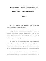
From a purely mechanical perspective, we need to calculate the present value of the
future cash flows at 15 percent. The net cash inflow will be $20,000 cash income less
$14,000 in costs per year for eight years. These cash flows are illustrated in Figure 9.1.
As Figure 9.1 suggests, we effectively have an eight-year annuity of $20,000 Ϫ 14,000 ϭ
$6,000 per year, along with a single lump sum inflow of $2,000 in eight years. Calculating
the present value of the future cash flows thus comes down to the same type of problem we

considered in Chapter 6. The total present value is:
Present value ϭ $6,000 ϫ [1 Ϫ (1͞1.158)]͞.15 ϩ (2,000͞1.158)
ϭ ($6,000 ϫ 4.4873) ϩ (2,000͞3.0590)
ϭ $26,924 ϩ 654
ϭ $27,578

ros3062x_Ch09.indd 266

2/9/07 11:19:49 AM


CHAPTER 9

Time (years)
Initial cost
Inflows
Outflows
Net inflow
Salvage
Net cash flow

0

267

Net Present Value and Other Investment Criteria

1

2

3

4

5

6

7

8

$ 20
Ϫ14
$ 6

$ 20
Ϫ14
$ 6

$ 20
Ϫ14
$ 6

$ 20
Ϫ14
$ 6

$ 20

Ϫ14
$ 6

$ 20
Ϫ14
$ 6

$ 20
Ϫ14
$ 6

$ 6

$ 6

$ 6

$ 6

$ 6

$ 6

$ 6

$ 20
Ϫ14
$ 6
2
$ 8

FIGURE 9.1
Project Cash Flows ($000)

Ϫ$30

Ϫ$30

When we compare this to the $30,000 estimated cost, we see that the NPV is:
NPV ϭ Ϫ$30,000 ϩ 27,578 ϭ Ϫ$2,422
Therefore, this is not a good investment. Based on our estimates, taking it would decrease
the total value of the stock by $2,422. With 1,000 shares outstanding, our best estimate of
the impact of taking this project is a loss of value of $2,422͞1,000 ϭ $2.42 per share.
Our fertilizer example illustrates how NPV estimates can be used to determine whether
an investment is desirable. From our example, notice that if the NPV is negative, the effect
on share value will be unfavorable. If the NPV were positive, the effect would be favorable. As a consequence, all we need to know about a particular proposal for the purpose of
making an accept–reject decision is whether the NPV is positive or negative.
Given that the goal of financial management is to increase share value, our discussion in
this section leads us to the net present value rule:
An investment should be accepted if the net present value is positive and rejected
if it is negative.

In the unlikely event that the net present value turned out to be exactly zero, we would be
indifferent between taking the investment and not taking it.
Two comments about our example are in order. First and foremost, it is not the rather
mechanical process of discounting the cash flows that is important. Once we have the cash
flows and the appropriate discount rate, the required calculations are fairly straightforward.
The task of coming up with the cash flows and the discount rate is much more challenging.
We will have much more to say about this in the next several chapters. For the remainder
of this chapter, we take it as a given that we have estimates of the cash revenues and costs

and, where needed, an appropriate discount rate.
The second thing to keep in mind about our example is that the Ϫ$2,422 NPV is an estimate. Like any estimate, it can be high or low. The only way to find out the true NPV would
be to place the investment up for sale and see what we could get for it. We generally won’t
be doing this, so it is important that our estimates be reliable. Once again, we will say more
about this later. For the rest of this chapter, we will assume the estimates are accurate.

Using the NPV Rule

EXAMPLE 9.1

Suppose we are asked to decide whether a new consumer product should be launched.
Based on projected sales and costs, we expect that the cash flows over the five-year life
of the project will be $2,000 in the first two years, $4,000 in the next two, and $5,000 in the
last year. It will cost about $10,000 to begin production. We use a 10 percent discount rate
to evaluate new products. What should we do here?
(continued )

ros3062x_Ch09.indd 267

2/9/07 11:19:50 AM


268

PA RT 4

Capital Budgeting

Given the cash flows and discount rate, we can calculate the total value of the product
by discounting the cash flows back to the present:

Present value ‫( ؍‬$2,000͞1.1) ؉ (2,000͞1.12) ؉ (4,000͞1.13)
؉ (4,000͞1.14) ؉ (5,000͞1.15)
‫ ؍‬$1,818 ؉ 1,653 ؉ 3,005 ؉ 2,732 ؉ 3,105
‫ ؍‬$12,313
The present value of the expected cash flows is $12,313, but the cost of getting those cash
flows is only $10,000, so the NPV is $12,313 ؊ 10,000 ‫ ؍‬$2,313. This is positive; so, based
on the net present value rule, we should take on the project.

As we have seen in this section, estimating NPV is one way of assessing the profitability
of a proposed investment. It is certainly not the only way profitability is assessed, and we
now turn to some alternatives. As we will see, when compared to NPV, each of the alternative ways of assessing profitability that we will examine is flawed in some key way; so
NPV is the preferred approach in principle, if not always in practice.

SPREADSHEET STRATEGIES
Calculating NPVs with a Spreadsheet
Spreadsheets are commonly used to calculate NPVs. Examining the use of spreadsheets in this context also
allows us to issue an important warning. Let’s rework Example 9.1:
A

B

C

D

E

F

G

H

1
2

You can get a
freeware NPV calculator
at www.wheatworks.com.

3
4
5
6
7
8
9
10
11
12
13
14
15
16
17
18
19
20
21

Using a spreadsheet to calculate net present values
From Example 9.1, the project’s cost is $10,000. The cash flows are $2,000 per year for the first
two years, $4,000 per year for the next two, and $5,000 in the last year. The discount rate is
10 percent; what’s the NPV?
Year
0
1
2
3
4
5

Cash Flow
-$10,000
2,000
2,000
4,000
4,000
5,000

Discount rate =
NPV =
NPV =

10%
$2,102.72 (wrong answer)
$2,312.99 (right answer)

The formula entered in cell F11 is =NPV(F9, C9:C14). This gives the wrong answer because the
NPV function actually calculates present values, not net present values.

The formula entered in cell F12 is =NPV(F9, C10:C14) + C9. This gives the right answer because the
NPV function is used to calculate the present value of the cash flows and then the initial cost is
subtracted to calculate the answer. Notice that we added cell C9 because it is already negative.

In our spreadsheet example, notice that we have provided two answers. By comparing the answers to that
found in Example 9.1, we see that the first answer is wrong even though we used the spreadsheet’s NPV formula.
What happened is that the “NPV” function in our spreadsheet is actually a PV function; unfortunately, one of the
original spreadsheet programs many years ago got the definition wrong, and subsequent spreadsheets have
copied it! Our second answer shows how to use the formula properly.
The example here illustrates the danger of blindly using calculators or computers without understanding what
is going on; we shudder to think of how many capital budgeting decisions in the real world are based on incorrect
use of this particular function. We will see another example of something that can go wrong with a spreadsheet
later in the chapter.

ros3062x_Ch09.indd 268

2/23/07 8:43:11 PM


CHAPTER 9

269

Net Present Value and Other Investment Criteria

Concept Questions
9.1a What is the net present value rule?
9.1b If we say an investment has an NPV of $1,000, what exactly do we mean?

The Payback Rule

9.2

It is common in practice to talk of the payback on a proposed investment. Loosely, the payback is the length of time it takes to recover our initial investment or “get our bait back.”
Because this idea is widely understood and used, we will examine it in some detail.

DEFINING THE RULE
We can illustrate how to calculate a payback with an example. Figure 9.2 shows the
cash flows from a proposed investment. How many years do we have to wait until the
accumulated cash flows from this investment equal or exceed the cost of the investment?
As Figure 9.2 indicates, the initial investment is $50,000. After the first year, the firm has
recovered $30,000, leaving $20,000. The cash flow in the second year is exactly $20,000,
so this investment “pays for itself” in exactly two years. Put another way, the payback
period is two years. If we require a payback of, say, three years or less, then this investment is acceptable. This illustrates the payback period rule:
Based on the payback rule, an investment is acceptable if its calculated payback
period is less than some prespecified number of years.

payback period
The amount of time
required for an investment
to generate cash flows
sufficient to recover its initial
cost.

In our example, the payback works out to be exactly two years. This won’t usually
happen, of course. When the numbers don’t work out exactly, it is customary to work with
fractional years. For example, suppose the initial investment is $60,000, and the cash flows
are $20,000 in the first year and $90,000 in the second. The cash flows over the first two
years are $110,000, so the project obviously pays back sometime in the second year. After
the first year, the project has paid back $20,000, leaving $40,000 to be recovered. To figure

Calculating Payback

EXAMPLE 9.2

Here are the projected cash flows from a proposed investment:
Year

Cash Flow

1
2
3

$100
200
500

This project costs $500. What is the payback period for this investment?
The initial cost is $500. After the first two years, the cash flows total $300. After the third
year, the total cash flow is $800, so the project pays back sometime between the end of
year 2 and the end of year 3. Because the accumulated cash flows for the first two years
are $300, we need to recover $200 in the third year. The third-year cash flow is $500, so
we will have to wait $200͞500 ‫ ؍‬.4 year to do this. The payback period is thus 2.4 years,
or about two years and five months.

ros3062x_Ch09.indd 269

2/9/07 11:19:57 AM

270

PA RT 4

FIGURE 9.2

Year

Net Project Cash Flows

TABLE 9.1
Expected Cash Flows
for Projects A
through E

Capital Budgeting

Year
0
1
2
3
4

0

1

2

3

4

Ϫ$50,000

$30,000

$20,000

$10,000

$5,000

A

B

C

D

؊$100
30
40
50
60

؊$200

40
20
10

؊$200
40
20
10
130

؊$200
100
100
؊200
200

E
؊$

50
100
؊50,000,000

out the fractional year, note that this $40,000 is $40,000͞90,000 ϭ 4͞9 of the second year’s
cash flow. Assuming that the $90,000 cash flow is received uniformly throughout the year,
the payback would be 14⁄9 years.
Now that we know how to calculate the payback period on an investment, using the
payback period rule for making decisions is straightforward. A particular cutoff time is
selected—say, two years—and all investment projects that have payback periods of two
years or less are accepted, whereas any that pay off in more than two years are rejected.

Table 9.1 illustrates cash flows for five different projects. The figures shown as the
Year 0 cash flows are the costs of the investments. We examine these to indicate some
peculiarities that can, in principle, arise with payback periods.
The payback for the first project, A, is easily calculated. The sum of the cash flows for
the first two years is $70, leaving us with $100 Ϫ 70 ϭ $30 to go. Because the cash flow
in the third year is $50, the payback occurs sometime in that year. When we compare the
$30 we need to the $50 that will be coming in, we get $30͞50 ϭ .6; so, payback will occur
60 percent of the way into the year. The payback period is thus 2.6 years.
Project B’s payback is also easy to calculate: It never pays back because the cash flows
never total up to the original investment. Project C has a payback of exactly four years
because it supplies the $130 that B is missing in year 4. Project D is a little strange. Because
of the negative cash flow in year 3, you can easily verify that it has two different payback
periods, two years and four years. Which of these is correct? Both of them; the way the
payback period is calculated doesn’t guarantee a single answer. Finally, Project E is obviously unrealistic, but it does pay back in six months, thereby illustrating the point that a
rapid payback does not guarantee a good investment.

ANALYZING THE RULE
When compared to the NPV rule, the payback period rule has some rather severe shortcomings. First, we calculate the payback period by simply adding up the future cash flows.
There is no discounting involved, so the time value of money is completely ignored. The
payback rule also fails to consider any risk differences. The payback would be calculated
the same way for both very risky and very safe projects.
Perhaps the biggest problem with the payback period rule is coming up with the right cutoff
period: We don’t really have an objective basis for choosing a particular number. Put another
way, there is no economic rationale for looking at payback in the first place, so we have no guide
for how to pick the cutoff. As a result, we end up using a number that is arbitrarily chosen.
Suppose we have somehow decided on an appropriate payback period of two years or
less. As we have seen, the payback period rule ignores the time value of money for the first

ros3062x_Ch09.indd 270

2/9/07 11:20:00 AM


CHAPTER 9

271

Net Present Value and Other Investment Criteria

Year

Long

Short

0
1
2
3
4

؊$250
100
100
100
100

؊$250
100
200

0
0

TABLE 9.2
Investment Projected
Cash Flows

two years. More seriously, cash flows after the second year are ignored entirely. To see this,
consider the two investments, Long and Short, in Table 9.2. Both projects cost $250. Based on
our discussion, the payback on Long is 2 ϩ ($50͞100) ϭ 2.5 years, and the payback on Short is
1 ϩ ($150͞200) ϭ 1.75 years. With a cutoff of two years, Short is acceptable and Long is not.
Is the payback period rule guiding us to the right decisions? Maybe not. Suppose we
require a 15 percent return on this type of investment. We can calculate the NPV for these
two investments as:
NPV(Short) ϭ Ϫ$250 ϩ (100͞1.15) ϩ (200͞1.152) ϭ Ϫ$11.81
NPV(Long) ϭ Ϫ$250 ϩ (100 ϫ {[1 Ϫ (1͞1.154)]͞.15}) ϭ $35.50
Now we have a problem. The NPV of the shorter-term investment is actually negative,
meaning that taking it diminishes the value of the shareholders’ equity. The opposite is true
for the longer-term investment—it increases share value.
Our example illustrates two primary shortcomings of the payback period rule. First,
by ignoring time value, we may be led to take investments (like Short) that actually are
worth less than they cost. Second, by ignoring cash flows beyond the cutoff, we may be
led to reject profitable long-term investments (like Long). More generally, using a payback
period rule will tend to bias us toward shorter-term investments.

REDEEMING QUALITIES OF THE RULE
Despite its shortcomings, the payback period rule is often used by large and sophisticated
companies when they are making relatively minor decisions. There are several reasons for
this. The primary reason is that many decisions simply do not warrant detailed analysis
because the cost of the analysis would exceed the possible loss from a mistake. As a practical matter, it can be said that an investment that pays back rapidly and has benefits extending beyond the cutoff period probably has a positive NPV.

Small investment decisions are made by the hundreds every day in large organizations.
Moreover, they are made at all levels. As a result, it would not be uncommon for a corporation to require, for example, a two-year payback on all investments of less than $10,000.
Investments larger than this would be subjected to greater scrutiny. The requirement of a
two-year payback is not perfect for reasons we have seen, but it does exercise some control
over expenditures and thus limits possible losses.
In addition to its simplicity, the payback rule has two other positive features. First,
because it is biased toward short-term projects, it is biased toward liquidity. In other words,
a payback rule tends to favor investments that free up cash for other uses quickly. This
could be important for a small business; it would be less so for a large corporation. Second,
the cash flows that are expected to occur later in a project’s life are probably more uncertain. Arguably, a payback period rule adjusts for the extra riskiness of later cash flows, but
it does so in a rather draconian fashion—by ignoring them altogether.
We should note here that some of the apparent simplicity of the payback rule is an illusion. The reason is that we still must come up with the cash flows first, and, as we discussed

ros3062x_Ch09.indd 271

2/9/07 11:20:03 AM


272

PA RT 4

Capital Budgeting

earlier, this is not at all easy to do. Thus, it would probably be more accurate to say that the
concept of a payback period is both intuitive and easy to understand.

SUMMARY OF THE RULE
To summarize, the payback period is a kind of “break-even” measure. Because time value
is ignored, you can think of the payback period as the length of time it takes to break even

in an accounting sense, but not in an economic sense. The biggest drawback to the payback
period rule is that it doesn’t ask the right question. The relevant issue is the impact an
investment will have on the value of the stock, not how long it takes to recover the initial
investment.
Nevertheless, because it is so simple, companies often use it as a screen for dealing
with the myriad minor investment decisions they have to make. There is certainly nothing wrong with this practice. As with any simple rule of thumb, there will be some errors
in using it; but it wouldn’t have survived all this time if it weren’t useful. Now that you
understand the rule, you can be on the alert for circumstances under which it might lead to
problems. To help you remember, the following table lists the pros and cons of the payback
period rule:
Advantages and Disadvantages of the Payback Period Rule
Advantages

Disadvantages

1. Easy to understand.
2. Adjusts for uncertainty of later
cash flows.
3. Biased toward liquidity.

1.
2.
3.
4.

Ignores the time value of money.
Requires an arbitrary cutoff point.
Ignores cash flows beyond the cutoff date.
Biased against long-term projects, such as
research and development, and new projects.

Concept Questions
9.2a In words, what is the payback period? The payback period rule?
9.2b Why do we say that the payback period is, in a sense, an accounting break-even
measure?

9.3 The Discounted Payback
discounted payback
period
The length of time required
for an investment’s
discounted cash flows to
equal its initial cost.

We saw that one shortcoming of the payback period rule was that it ignored time value. A
variation of the payback period, the discounted payback period, fixes this particular problem. The discounted payback period is the length of time until the sum of the discounted
cash flows is equal to the initial investment. The discounted payback rule would be:
Based on the discounted payback rule, an investment is acceptable if its
discounted payback is less than some prespecified number of years.

To see how we might calculate the discounted payback period, suppose we require
a 12.5 percent return on new investments. We have an investment that costs $300 and

ros3062x_Ch09.indd 272

2/9/07 11:20:04 AM


CHAPTER 9

Cash Flow

Accumulated Cash Flow

Year

Undiscounted

Discounted

Undiscounted

Discounted

1
2
3
4

$100
100
100

$89
79
70

$100
200
300

$ 89
168
238

100
100

62
55

400
500

300
355

5

273

Net Present Value and Other Investment Criteria

TABLE 9.3
Ordinary and Discounted
Payback

has cash flows of $100 per year for five years. To get the discounted payback, we have to
discount each cash flow at 12.5 percent and then start adding them. We do this in Table 9.3.
In Table 9.3, we have both the discounted and the undiscounted cash flows. Looking at the

accumulated cash flows, we see that the regular payback is exactly three years (look for
the highlighted figure in year 3). The discounted cash flows total $300 only after four years,
however, so the discounted payback is four years, as shown.1
How do we interpret the discounted payback? Recall that the ordinary payback is the
time it takes to break even in an accounting sense. Because it includes the time value of
money, the discounted payback is the time it takes to break even in an economic or financial sense. Loosely speaking, in our example, we get our money back, along with the interest we could have earned elsewhere, in four years.
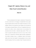
Figure 9.3 illustrates this idea by comparing the future value at 12.5 percent of the $300
investment to the future value of the $100 annual cash flows at 12.5 percent. Notice that the
two lines cross at exactly four years. This tells us that the value of the project’s cash flows
catches up and then passes the original investment in four years.
Table 9.3 and Figure 9.3 illustrate another interesting feature of the discounted payback
period. If a project ever pays back on a discounted basis, then it must have a positive NPV.2
This is true because, by definition, the NPV is zero when the sum of the discounted cash
flows equals the initial investment. For example, the present value of all the cash flows in
Table 9.3 is $355. The cost of the project was $300, so the NPV is obviously $55. This $55
is the value of the cash flow that occurs after the discounted payback (see the last line in
Table 9.3). In general, if we use a discounted payback rule, we won’t accidentally take any
projects with a negative estimated NPV.
Based on our example, the discounted payback would seem to have much to recommend it. You may be surprised to find out that it is rarely used in practice. Why? Probably
because it really isn’t any simpler to use than NPV. To calculate a discounted payback, you
have to discount cash flows, add them up, and compare them to the cost, just as you do with
NPV. So, unlike an ordinary payback, the discounted payback is not especially simple to
calculate.
A discounted payback period rule has a couple of other significant drawbacks. The
biggest one is that the cutoff still has to be arbitrarily set, and cash flows beyond that point
are ignored.3 As a result, a project with a positive NPV may be found unacceptable because

1

In this case, the discounted payback is an even number of years. This won’t ordinarily happen, of course. However, calculating a fractional year for the discounted payback period is more involved than it is for the ordinary

payback, and it is not commonly done.
2
This argument assumes the cash flows, other than the first, are all positive. If they are not, then these statements
are not necessarily correct. Also, there may be more than one discounted payback.
3
If the cutoff were forever, then the discounted payback rule would be the same as the NPV rule. It would also
be the same as the profitability index rule considered in a later section.

ros3062x_Ch09.indd 273

2/9/07 11:20:05 AM


274

PA RT 4

Capital Budgeting

FIGURE 9.3
Future Value of Project
Cash Flows

700
$642
600
Future value ($)

$541
500

$ 4 81

FV of initial investment
400
300

FV of projected cash flow
200
100

0

1

2

3
Year

5

4

Future Value at 12.5%
Year

$100 Annuity
(Projected Cash Flow)

$300 Lump Sum

(Projected Investment)

0
1
2
3
4
5

$ 0
100
213
339
481
642

$300
338
380
427
481
541

the cutoff is too short. Also, just because one project has a shorter discounted payback than
another does not mean it has a larger NPV.
All things considered, the discounted payback is a compromise between a regular payback and NPV that lacks the simplicity of the first and the conceptual rigor of the second.
Nonetheless, if we need to assess the time it will take to recover the investment required
by a project, then the discounted payback is better than the ordinary payback because it
considers time value. In other words, the discounted payback recognizes that we could
have invested the money elsewhere and earned a return on it. The ordinary payback does

not take this into account. The advantages and disadvantages of the discounted payback
rule are summarized in the following table:

Advantages and Disadvantages of the Discounted Payback Period Rule

ros3062x_Ch09.indd 274

Advantages

Disadvantages

1. Includes time value of money.
2. Easy to understand.
3. Does not accept negative estimated
NPV investments.
4. Biased toward liquidity.

1.
2.
3.
4.

May reject positive NPV investments.
Requires an arbitrary cutoff point.
Ignores cash flows beyond the cutoff date.
Biased against long-term projects, such as
research and development, and new projects.

2/9/07 11:20:06 AM

CHAPTER 9

275

Net Present Value and Other Investment Criteria

Calculating Discounted Payback

EXAMPLE 9.3

Consider an investment that costs $400 and pays $100 per year forever. We use a 20 percent discount rate on this type of investment. What is the ordinary payback? What is the
discounted payback? What is the NPV?
The NPV and ordinary payback are easy to calculate in this case because the investment is a perpetuity. The present value of the cash flows is $100͞.2 ϭ $500, so the NPV is
$500 Ϫ 400 ϭ $100. The ordinary payback is obviously four years.
To get the discounted payback, we need to find the number of years such that a $100
annuity has a present value of $400 at 20 percent. In other words, the present value annuity
factor is $400͞100 ϭ 4, and the interest rate is 20 percent per period; so what’s the number
of periods? If we solve for the number of periods, we find that the answer is a little less than
nine years, so this is the discounted payback.

Concept Questions
9.3a In words, what is the discounted payback period? Why do we say it is, in a
sense, a financial or economic break-even measure?
9.3b What advantage(s) does the discounted payback have over the ordinary
payback?

The Average Accounting Return

9.4

Another attractive, but flawed, approach to making capital budgeting decisions involves
the average accounting return (AAR). There are many different definitions of the AAR.
However, in one form or another, the AAR is always defined as:
Some measure of average accounting profit
____________________________________
Some measure of average accounting value
The specific definition we will use is:
Average
net income
_________________
Average book value
To see how we might calculate this number, suppose we are deciding whether to open
a store in a new shopping mall. The required investment in improvements is $500,000.
The store would have a five-year life because everything reverts to the mall owners after
that time. The required investment would be 100 percent depreciated (straight-line) over
five years, so the depreciation would be $500,000͞5 ϭ $100,000 per year. The tax rate is
25 percent. Table 9.4 contains the projected revenues and expenses. Net income in each
year, based on these figures, is also shown.
To calculate the average book value for this investment, we note that we started out with a
book value of $500,000 (the initial cost) and ended up at $0. The average book value during
the life of the investment is thus ($500,000 ϩ 0)͞2 ϭ $250,000. As long as we use straightline depreciation, the average investment will always be one-half of the initial investment.4

average accounting
return (AAR)
An investment’s average
net income divided by its
average book value.

4

We could, of course, calculate the average of the six book values directly. In thousands, we would have
($500 ϩ 400 ϩ 300 ϩ 200 ϩ 100 ϩ 0)͞6 ϭ $250.

ros3062x_Ch09.indd 275

2/9/07 11:20:06 AM


276

PA RT 4

Capital Budgeting

TABLE 9.4
Projected Yearly Revenue
and Costs for Average
Accounting Return

Revenue
Expenses
Earnings before Depreciation
Depreciation
Earnings before Taxes
Taxes (25%)
Net Income

Year 1

Year 2

Year 3

Year 4

Year 5

$433,333
$200,000
$233,333
$100,000
$133,333
33,333
$100,000

$450,000
$150,000
$300,000
$100,000
$200,000
50,000
$150,000

$266,667
$100,000
$166,667
$100,000
$ 66,667
16,667

$ 50,000

$200,000
$100,000
$100,000
$100,000
$
0
0
$
0

$133,333
$100,000
$ 33,333
$100,000
؊$ 66,667
؊ 16,667
؊$ 50,000

$100,000 ؉ 150,000 ؉ 50,000 ؉ 0 ؊ 50,000
Average net income ‫ ؍ _________________________________________ ؍‬$50,000
5
$500,000 ؉ 0
Average book value ‫ ؍ _____________ ؍‬$250,000
2

Looking at Table 9.4, we see that net income is $100,000 in the first year, $150,000 in
the second year, $50,000 in the third year, $0 in Year 4, and Ϫ$50,000 in Year 5. The average net income, then, is:
[$100,000 ϩ 150,000 ϩ 50,000 ϩ 0 ϩ (Ϫ50,000)]͞5 ϭ $50,000

The average accounting return is:
Average net income
$50,000
AARϭ ______________ ϭ ________ ϭ 20%
Average book value $250,000
If the firm has a target AAR of less than 20 percent, then this investment is acceptable;
otherwise it is not. The average accounting return rule is thus:
Based on the average accounting return rule, a project is acceptable if its average
accounting return exceeds a target average accounting return.

As we will now see, the use of this rule has a number of problems.
You should recognize the chief drawback to the AAR immediately. Above all else, the
AAR is not a rate of return in any meaningful economic sense. Instead, it is the ratio of
two accounting numbers, and it is not comparable to the returns offered, for example, in
financial markets.5
One of the reasons the AAR is not a true rate of return is that it ignores time value. When
we average figures that occur at different times, we are treating the near future and the more
distant future in the same way. There was no discounting involved when we computed the
average net income, for example.
The second problem with the AAR is similar to the problem we had with the payback
period rule concerning the lack of an objective cutoff period. Because a calculated AAR
is really not comparable to a market return, the target AAR must somehow be specified.
There is no generally agreed-upon way to do this. One way of doing it is to calculate the
AAR for the firm as a whole and use this as a benchmark, but there are lots of other ways
as well.

5

The AAR is closely related to the return on assets (ROA) discussed in Chapter 3. In practice, the AAR is sometimes computed by first calculating the ROA for each year and then averaging the results. This produces
a number that is similar, but not identical, to the one we computed.

ros3062x_Ch09.indd 276

2/9/07 11:20:07 AM


CHAPTER 9

277

Net Present Value and Other Investment Criteria

The third, and perhaps worst, flaw in the AAR is that it doesn’t even look at the right
things. Instead of cash flow and market value, it uses net income and book value. These are
both poor substitutes. As a result, an AAR doesn’t tell us what the effect on share price will
be of taking an investment, so it doesn’t tell us what we really want to know.
Does the AAR have any redeeming features? About the only one is that it almost always
can be computed. The reason is that accounting information will almost always be available, both for the project under consideration and for the firm as a whole. We hasten to add
that once the accounting information is available, we can always convert it to cash flows,
so even this is not a particularly important fact. The AAR is summarized in the following
table:
Advantages and Disadvantages of the Average Accounting Return
Advantages

Disadvantages

1. Easy to calculate.
2. Needed information will usually
be available.

1. Not a true rate of return; time value of money
is ignored.
2. Uses an arbitrary benchmark cutoff rate.
3. Based on accounting (book) values, not cash
flows and market values.

Concept Questions
9.4a What is an average accounting rate of return (AAR)?
9.4b What are the weaknesses of the AAR rule?

The Internal Rate of Return

9.5

We now come to the most important alternative to NPV, the internal rate of return, universally known as the IRR. As we will see, the IRR is closely related to NPV. With the
IRR, we try to find a single rate of return that summarizes the merits of a project. Furthermore, we want this rate to be an “internal” rate in the sense that it depends only on the cash
flows of a particular investment, not on rates offered elsewhere.
To illustrate the idea behind the IRR, consider a project that costs $100 today and pays
$110 in one year. Suppose you were asked, “What is the return on this investment?” What
would you say? It seems both natural and obvious to say that the return is 10 percent
because, for every dollar we put in, we get $1.10 back. In fact, as we will see in a moment,
10 percent is the internal rate of return, or IRR, on this investment.
Is this project with its 10 percent IRR a good investment? Once again, it would seem
apparent that this is a good investment only if our required return is less than 10 percent.
This intuition is also correct and illustrates the IRR rule:

internal rate of return
(IRR)
The discount rate that
makes the NPV of an

investment zero.

Based on the IRR rule, an investment is acceptable if the IRR exceeds the
required return. It should be rejected otherwise.

Imagine that we want to calculate the NPV for our simple investment. At a discount rate
of R, the NPV is:
NPV ϭ Ϫ$100 ϩ [110͞(1 ϩ R)]

ros3062x_Ch09.indd 277

2/9/07 11:20:08 AM


278

PA RT 4

Capital Budgeting

Now, suppose we don’t know the discount rate. This presents a problem, but we can still
ask how high the discount rate would have to be before this project was deemed unacceptable. We know that we are indifferent between taking and not taking this investment when its NPV is just equal to zero. In other words, this investment is economically
a break-even proposition when the NPV is zero because value is neither created nor
destroyed. To find the break-even discount rate, we set NPV equal to zero and solve
for R:
NPV ϭ 0 ϭ Ϫ$100 ϩ [110͞(1 ϩ R)]
$100 ϭ $110͞(1 ϩ R)
1 ϩ R ϭ $110͞100 ϭ 1.1
R ϭ 10%
This 10 percent is what we already have called the return on this investment. What we have

now illustrated is that the internal rate of return on an investment (or just “return” for short)
is the discount rate that makes the NPV equal to zero. This is an important observation, so
it bears repeating:
The IRR on an investment is the required return that results in a zero NPV
when it is used as the discount rate.

The fact that the IRR is simply the discount rate that makes the NPV equal to zero is
important because it tells us how to calculate the returns on more complicated investments. As we have seen, finding the IRR turns out to be relatively easy for a singleperiod investment. However, suppose you were now looking at an investment with the
cash flows shown in Figure 9.4. As illustrated, this investment costs $100 and has a
cash flow of $60 per year for two years, so it’s only slightly more complicated than our
single-period example. However, if you were asked for the return on this investment,
what would you say? There doesn’t seem to be any obvious answer (at least not to us).
However, based on what we now know, we can set the NPV equal to zero and solve for
the discount rate:
NPV ϭ 0 ϭ Ϫ$100 ϩ [60͞(1 ϩ IRR)] ϩ [60͞(1 ϩ IRR)2]
Unfortunately, the only way to find the IRR in general is by trial and error, either by hand
or by calculator. This is precisely the same problem that came up in Chapter 5 when we
found the unknown rate for an annuity and in Chapter 7 when we found the yield to maturity on a bond. In fact, we now see that in both of those cases, we were finding an IRR.
In this particular case, the cash flows form a two-period, $60 annuity. To find the
unknown rate, we can try some different rates until we get the answer. If we were to start
with a 0 percent rate, the NPV would obviously be $120 Ϫ 100 ϭ $20. At a 10 percent
discount rate, we would have:
NPV ϭ Ϫ$100 ϩ (60͞1.1) ϩ (60͞1.12) ϭ $4.13
FIGURE 9.4
Project Cash Flows

Year

0
Ϫ$100

ros3062x_Ch09.indd 278

1
ϩ$60

2
ϩ$60

2/9/07 11:20:09 AM


CHAPTER 9

279

Net Present Value and Other Investment Criteria

Discount Rate

TABLE 9.5

NPV

0%
5%
10%
15%
20%

NPV at Different
Discount Rates

$20.00
11.56
4.13
؊ 2.46
؊ 8.33

FIGURE 9.5
An NPV Profile
20
15

NPV ($)

10
5
0
Ϫ5

IRR ϭ 13.1%

NPV Ͼ 0
5

10

15

20

25

30

R(%)

NPV Ͻ 0

Ϫ10

Now, we’re getting close. We can summarize these and some other possibilities as shown in
Table 9.5. From our calculations, the NPV appears to be zero with a discount rate between
10 percent and 15 percent, so the IRR is somewhere in that range. With a little more effort, we
can find that the IRR is about 13.1 percent.6 So, if our required return were less than 13.1 percent,
we would take this investment. If our required return exceeded 13.1 percent, we would reject it.
By now, you have probably noticed that the IRR rule and the NPV rule appear to be
quite similar. In fact, the IRR is sometimes simply called the discounted cash flow, or DCF,
return. The easiest way to illustrate the relationship between NPV and IRR is to plot the
numbers we calculated for Table 9.5. We put the different NPVs on the vertical axis, or
y-axis, and the discount rates on the horizontal axis, or x-axis. If we had a very large number of points, the resulting picture would be a smooth curve called a net present value
profile. Figure 9.5 illustrates the NPV profile for this project. Beginning with a 0 percent
discount rate, we have $20 plotted directly on the y-axis. As the discount rate-increases,
the NPV declines smoothly. Where will the curve cut through the x-axis? This will occur
where the NPV is just equal to zero, so it will happen right at the IRR of 13.1 percent.
In our example, the NPV rule and the IRR rule lead to identical accept–reject decisions. We will accept an investment using the IRR rule if the required return is less than
13.1 percent. As Figure 9.5 illustrates, however, the NPV is positive at any discount rate
less than 13.1 percent, so we would accept the investment using the NPV rule as well. The
two rules give equivalent results in this case.

net present value
profile
A graphical representation
of the relationship between
an investment’s NPVs and
various discount rates.

6

With a lot more effort (or a personal computer), we can find that the IRR is approximately (to 9 decimal places)
13.066238629 percent—not that anybody would ever want this many decimal places!

ros3062x_Ch09.indd 279

2/9/07 11:20:10 AM


280

PA RT 4

EXAMPLE 9.4

Capital Budgeting

Calculating the IRR
A project has a total up-front cost of $435.44. The cash flows are $100 in the first year,
$200 in the second year, and $300 in the third year. What’s the IRR? If we require an
18 percent return, should we take this investment?

We’ll describe the NPV profile and find the IRR by calculating some NPVs at different discount rates. You should check our answers for practice. Beginning with 0 percent, we have:
Discount Rate

NPV

0%
5%
10%
15%
20%

$164.56
100.36
46.15
0.00
Ϫ 39.61

The NPV is zero at 15 percent, so 15 percent is the IRR. If we require an 18 percent return,
then we should not take the investment. The reason is that the NPV is negative at 18 percent
(verify that it is ؊$24.47). The IRR rule tells us the same thing in this case. We shouldn’t take
this investment because its 15 percent return is below our required 18 percent return.

At this point, you may be wondering if the IRR and NPV rules always lead to identical decisions. The answer is yes, as long as two very important conditions are met. First,
the project’s cash flows must be conventional, meaning that the first cash flow (the initial
investment) is negative and all the rest are positive. Second, the project must be independent, meaning that the decision to accept or reject this project does not affect the decision
to accept or reject any other. The first of these conditions is typically met, but the second
often is not. In any case, when one or both of these conditions are not met, problems can
arise. We discuss some of these next.

SPREADSHEET STRATEGIES

Calculating IRRs with a Spreadsheet
Because IRRs are so tedious to calculate by hand, financial calculators and especially spreadsheets are generally
used. The procedures used by various financial calculators are too different for us to illustrate here, so we will
focus on using a spreadsheet (financial calculators are covered in Appendix D). As the following example illustrates, using a spreadsheet is easy.
A

B

C

D

E

F

G

H

1
2
3
4
5
6
7
8
9
10

11
12
13
14
15
16
17

ros3062x_Ch09.indd 280

Using a spreadsheet to calculate internal rates of return
Suppose we have a four-year project that costs $500. The cash flows over the four-year life will be
$100, $200, $300, and $400. What is the IRR?
Year
0
1
2
3
4

Cash Flow
-$500
100
200
300
400

IRR =

27.3%

The formula entered in cell F9 is =IRR(C8:C12). Notice that the year 0 cash flow has a negative
sign representing the initial cost of the project.

2/9/07 11:20:11 AM


CHAPTER 9

281

Net Present Value and Other Investment Criteria

PROBLEMS WITH THE IRR
The problems with the IRR come about when the cash flows are not conventional or when
we are trying to compare two or more investments to see which is best. In the first case,
surprisingly, the simple question: What’s the return? can become difficult to answer. In the
second case, the IRR can be a misleading guide.

Nonconventional Cash Flows Suppose we have a strip-mining project that requires a
$60 investment. Our cash flow in the first year will be $155. In the second year, the mine
will be depleted, but we will have to spend $100 to restore the terrain. As Figure 9.6 illustrates, both the first and third cash flows are negative.
To find the IRR on this project, we can calculate the NPV at various rates:
Discount Rate

NPV
Ϫ$5.00
Ϫ 1.74
Ϫ 0.28
0.06

Ϫ 0.31

0%
10%
20%
30%
40%

The NPV appears to be behaving in a peculiar fashion here. First, as the discount rate
increases from 0 percent to 30 percent, the NPV starts out negative and becomes positive.
This seems backward because the NPV is rising as the discount rate rises. It then starts getting smaller and becomes negative again. What’s the IRR? To find out, we draw the NPV
profile as shown in Figure 9.7.
In Figure 9.7, notice that the NPV is zero when the discount rate is 25 percent, so this
is the IRR. Or is it? The NPV is also zero at 33_13 percent. Which of these is correct? The
answer is both or neither; more precisely, there is no unambiguously correct answer. This
is the multiple rates of return problem. Many financial computer packages (including a
best-seller for personal computers) aren’t aware of this problem and just report the first
IRR that is found. Others report only the smallest positive IRR, even though this answer is
no better than any other.
In our current example, the IRR rule breaks down completely. Suppose our required
return is 10 percent. Should we take this investment? Both IRRs are greater than 10 percent, so, by the IRR rule, maybe we should. However, as Figure 9.7 shows, the NPV is
negative at any discount rate less than 25 percent, so this is not a good investment. When
should we take it? Looking at Figure 9.7 one last time, we see that the NPV is positive only
if our required return is between 25 percent and 33_13 percent.
Nonconventional cash flows can occur in a variety of ways. For example, Northeast
Utilities, owner of the Connecticut-located Millstone nuclear power plant, had to shut
down the plant’s three reactors in November 1995. The reactors were expected to be back
online in January 1997. By some estimates, the cost of the shutdown would run about
$334 million. In fact, all nuclear plants eventually have to be shut down forever, and the
costs associated with decommissioning a plant are enormous, creating large negative cash

flows at the end of the project’s life.
Year

0
Ϫ$60

ros3062x_Ch09.indd 281

1
ϩ$155

2

multiple rates of return
The possibility that more
than one discount rate
will make the NPV of an
investment zero.

FIGURE 9.6
Project Cash Flows

Ϫ$100

2/9/07 11:20:13 AM


282

PA RT 4

Capital Budgeting

FIGURE 9.7
NPV Prof ile

2

1

NPV ($)

0

1

IRR ϭ 25%

10

20

IRR ϭ 33 3%

30

40

50

R(%)

Ϫ1

Ϫ2

Ϫ3

Ϫ4

Ϫ5

The moral of the story is that when the cash flows aren’t conventional, strange
things can start to happen to the IRR. This is not anything to get upset about, however,
because the NPV rule, as always, works just fine. This illustrates the fact that, oddly
enough, the obvious question—What’s the rate of return?—may not always have a
good answer.

EXAMPLE 9.5

What’s the IRR?
You are looking at an investment that requires you to invest $51 today. You’ll get
$100 in one year, but you must pay out $50 in two years. What is the IRR on this
investment?
You’re on the alert now for the nonconventional cash flow problem, so you probably wouldn’t be surprised to see more than one IRR. However, if you start looking for
an IRR by trial and error, it will take you a long time. The reason is that there is no IRR.
The NPV is negative at every discount rate, so we shouldn’t take this investment under any circumstances. What’s the return on this investment? Your guess is as good
as ours.

ros3062x_Ch09.indd 282

2/9/07 11:20:15 AM


CHAPTER 9

283

Net Present Value and Other Investment Criteria

“I Think; Therefore, I Know How Many IRRs There Can Be.”

EXAMPLE 9.6

We’ve seen that it’s possible to get more than one IRR. If you wanted to make sure that
you had found all of the possible IRRs, how could you do it? The answer comes from the
great mathematician, philosopher, and financial analyst Descartes (of “I think; therefore
I am” fame). Descartes’ Rule of Sign says that the maximum number of IRRs that there can
be is equal to the number of times that the cash flows change sign from positive to negative and/or negative to positive.7
In our example with the 25 percent and 331⁄3 percent IRRs, could there be yet another
IRR? The cash flows flip from negative to positive, then back to negative, for a total of two
sign changes. Therefore, according to Descartes’ rule, the maximum number of IRRs is two
and we don’t need to look for any more. Note that the actual number of IRRs can be less
than the maximum (see Example 9.5).

Mutually Exclusive Investments Even if there is a single IRR, another problem can
arise concerning mutually exclusive investment decisions. If two investments, X and Y,
are mutually exclusive, then taking one of them means that we cannot take the other. Two
projects that are not mutually exclusive are said to be independent. For example, if we own
one corner lot, then we can build a gas station or an apartment building, but not both. These

are mutually exclusive alternatives.
Thus far, we have asked whether a given investment is worth undertaking. However, a
related question comes up often: Given two or more mutually exclusive investments, which
one is the best? The answer is simple enough: The best one is the one with the largest NPV. Can
we also say that the best one has the highest return? As we show, the answer is no.
To illustrate the problem with the IRR rule and mutually exclusive investments, consider the following cash flows from two mutually exclusive investments:
Year

Investment A
؊$100
50
40
40
30

0
1
2
3
4

mutually exclusive
investment decisions
A situation in which taking
one investment prevents
the taking of another.

Investment B
؊$100
20

40
50
60

The IRR for A is 24 percent, and the IRR for B is 21 percent. Because these investments are
mutually exclusive, we can take only one of them. Simple intuition suggests that investment
A is better because of its higher return. Unfortunately, simple intuition is not always correct.
To see why investment A is not necessarily the better of the two investments, we’ve
calculated the NPV of these investments for different required returns:
Discount Rate

NPV(A)

0%
5
10
15
20
25

$60.00
43.13
29.06
17.18
7.06
؊ 1.63

NPV(B)
$70.00
47.88

29.79
14.82
2.31
؊ 8.22

To be more precise, the number of IRRs that are bigger than Ϫ100 percent is equal to the number of sign changes,
or it differs from the number of sign changes by an even number. Thus, for example, if there are five sign changes,
there are five IRRs, three IRRs, or one IRR. If there are two sign changes, there are either two IRRs or no IRRs.

7

ros3062x_Ch09.indd 283

2/9/07 11:20:16 AM


284

PA RT 4

Capital Budgeting

FIGURE 9.8
NPV Profiles for Mutually
Exclusive Investments

70
60
50
Investment B

NPV ($)

40
Investment A

Crossover point

30
26.34
20
10

NPVB Ͼ NPVA

IRRA ϭ 24%

NPVA Ͼ NPVB
0
Ϫ10

5

10
11.1%

15

20

25

30

R(%)

IRRB ϭ 21%

The IRR for A (24 percent) is larger than the IRR for B (21 percent). However, if you
compare the NPVs, you’ll see that which investment has the higher NPV depends on our
required return. B has greater total cash flow, but it pays back more slowly than A. As a
result, it has a higher NPV at lower discount rates.
In our example, the NPV and IRR rankings conflict for some discount rates. If our
required return is 10 percent, for instance, then B has the higher NPV and is thus the better
of the two even though A has the higher return. If our required return is 15 percent, then
there is no ranking conflict: A is better.
The conflict between the IRR and NPV for mutually exclusive investments can be illustrated by plotting the investments’ NPV profiles as we have done in Figure 9.8. In Figure 9.8,
notice that the NPV profiles cross at about 11 percent. Notice also that at any discount rate
less than 11 percent, the NPV for B is higher. In this range, taking B benefits us more than
taking A, even though A’s IRR is higher. At any rate greater than 11 percent, investment A
has the greater NPV.
This example illustrates that when we have mutually exclusive projects, we shouldn’t
rank them based on their returns. More generally, anytime we are comparing investments
to determine which is best, looking at IRRs can be misleading. Instead, we need to look at
the relative NPVs to avoid the possibility of choosing incorrectly. Remember, we’re ultimately interested in creating value for the shareholders, so the option with the higher NPV
is preferred, regardless of the relative returns.
If this seems counterintuitive, think of it this way. Suppose you have two investments. One has a 10 percent return and makes you $100 richer immediately. The other
has a 20 percent return and makes you $50 richer immediately. Which one do you like
better? We would rather have $100 than $50, regardless of the returns, so we like the
first one better.

ros3062x_Ch09.indd 284

2/9/07 11:20:16 AM


CHAPTER 9

285

Net Present Value and Other Investment Criteria

Calculating the Crossover Rate

EXAMPLE 9.7

In Figure 9.8, the NPV profiles cross at about 11 percent. How can we determine just what
this crossover point is? The crossover rate, by definition, is the discount rate that makes
the NPVs of two projects equal. To illustrate, suppose we have the following two mutually
exclusive investments:
Year

Investment A

Investment B

0
1
2

؊$400

250
280

؊$500
320
340

What’s the crossover rate?
To find the crossover, first consider moving out of investment A and into investment B. If
you make the move, you’ll have to invest an extra $100 (‫ ؍‬$500 ؊ 400). For this $100 investment, you’ll get an extra $70 (‫ ؍‬$320 ؊ 250) in the first year and an extra $60 (‫ ؍‬$340 ؊ 280) in
the second year. Is this a good move? In other words, is it worth investing the extra $100?
Based on our discussion, the NPV of the switch, NPV(B ؊ A), is:
NPV(B ؊ A) ‫ ؍‬؊$100 ؉ [70͞(1 ؉ R)] ؉ [60͞(1 ؉ R)2]
We can calculate the return on this investment by setting the NPV equal to zero and solving
for the IRR:
NPV(B ؊ A) ‫ ؍‬0 ‫ ؍‬؊$100 ؉ [70͞(1 ؉ R)] ؉ [60͞(1 ؉ R)2]
If you go through this calculation, you will find the IRR is exactly 20 percent. What this tells
us is that at a 20 percent discount rate, we are indifferent between the two investments
because the NPV of the difference in their cash flows is zero. As a consequence, the two
investments have the same value, so this 20 percent is the crossover rate. Check to see
that the NPV at 20 percent is $2.78 for both investments.
In general, you can find the crossover rate by taking the difference in the cash flows
and calculating the IRR using the difference. It doesn’t make any difference which one
you subtract from which. To see this, find the IRR for (A ؊ B); you’ll see it’s the same number. Also, for practice, you might want to find the exact crossover in Figure 9.8. (Hint: It’s
11.0704 percent.)

REDEEMING QUALITIES OF THE IRR
Despite its flaws, the IRR is very popular in practice—more so than even the NPV. It
probably survives because it fills a need that the NPV does not. In analyzing investments,
people in general, and financial analysts in particular, seem to prefer talking about rates of

return rather than dollar values.
In a similar vein, the IRR also appears to provide a simple way of communicating
information about a proposal. One manager might say to another, “Remodeling the clerical wing has a 20 percent return.” This may somehow seem simpler than saying, “At a
10 percent discount rate, the net present value is $4,000.”
Finally, under certain circumstances, the IRR may have a practical advantage over the
NPV. We can’t estimate the NPV unless we know the appropriate discount rate, but we
can still estimate the IRR. Suppose we didn’t know the required return on an investment,
but we found, for example, that it had a 40 percent return. We would probably be inclined
to take it because it would be unlikely that the required return would be that high. The

ros3062x_Ch09.indd 285

2/9/07 11:20:17 AM


286

PA RT 4

Capital Budgeting

advantages and disadvantages of the IRR are summarized as follows:
Advantages and Disadvantages of the Internal Rate of Return
Advantages

Disadvantages

1. Closely related to NPV, often leading to
identical decisions.
2. Easy to understand and communicate.

1. May result in multiple answers or not deal
with nonconventional cash flows.
2. May lead to incorrect decisions in comparisons of mutually exclusive investments.

THE MODIFIED INTERNAL RATE OF RETURN (MIRR)
To address some of the problems that can crop up with the standard IRR, it is often proposed that a modified version be used. As we will see, there are several different ways of
calculating a modified IRR, or MIRR, but the basic idea is to modify the cash flows first
and then calculate an IRR using the modified cash flows.
To illustrate, let’s go back to the cash flows in Figure 9.6: Ϫ$60, ϩ$155, and Ϫ$100.
As we saw, there are two IRRs, 25 percent and 33_13 percent. We next illustrate three different MIRRs, all of which have the property that only one answer will result, thereby
eliminating the multiple IRR problem.

Method #1: The Discounting Approach With the discounting approach, the idea is to
discount all negative cash flows back to the present at the required return and add them to
the initial cost. Then, calculate the IRR. Because only the first modified cash flow is negative, there will be only one IRR. The discount rate used might be the required return, or it
might be some other externally supplied rate. We will use the project’s required return.
If the required return on the project is 20 percent, then the modified cash flows look like this:
Time 0:
Time 1:
Time 2:

Ϫ$100
Ϫ$60 ϩ ______
ϭ Ϫ$129.44
1.202
ϩ$155
ϩ$0

If you calculate the MIRR now, you should get 19.71 percent.

Method #2: The Reinvestment Approach With the reinvestment approach, we compound all cash flows (positive and negative) except the first out to the end of the project’s
life and then calculate the IRR. In a sense, we are “reinvesting” the cash flows and not taking
them out of the project until the very end. The rate we use could be the required return on the
project, or it could be a separately specified “reinvestment rate.” We will use the project’s
required return. When we do, here are the modified cash flows:
Time 0:
Time 1:
Time 2:

Ϫ$60
ϩ0
Ϫ$100 ϩ ($155 ϫ 1.2) ϭ $86

The MIRR on this set of cash flows is 19.72 percent, or a little higher than we got using the
discounting approach.

Method #3: The Combination Approach As the name suggests, the combination approach
blends our first two methods. Negative cash flows are discounted back to the present, and positive cash flows are compounded to the end of the project. In practice, different discount or
compounding rates might be used, but we will again stick with the project’s required return.

ros3062x_Ch09.indd 286

2/9/07 11:20:17 AM


CHAPTER 9

287

Net Present Value and Other Investment Criteria

With the combination approach, the modified cash flows are as follows:
Time 0:
Time 1:
Time 2:

Ϫ$100
Ϫ$60 ϩ ______
ϭ Ϫ$129.44
1.202
ϩ0
$155 ϫ 1.2 ϭ $186

See if you don’t agree that the MIRR is 19.87 percent, the highest of the three.

MIRR or IRR: Which Is Better? MIRRs are controversial. At one extreme are those who
claim that MIRRs are superior to IRRs, period. For example, by design, they clearly don’t
suffer from the multiple rate of return problem.
At the other end, detractors say that MIRR should stand for “meaningless internal rate
of return.” As our example makes clear, one problem with MIRRs is that there are different
ways of calculating them, and there is no clear reason to say one of our three methods is
better than any other. The differences are small with our simple cash flows, but they could
be much larger for a more complex project. Further, it’s not clear how to interpret an MIRR.
It may look like a rate of return; but it’s a rate of return on a modified set of cash flows, not
the project’s actual cash flows.
We’re not going to take sides. However, notice that calculating an MIRR requires
discounting, compounding, or both, which leads to two obvious observations. First, if we
have the relevant discount rate, why not calculate the NPV and be done with it? Second,
because an MIRR depends on an externally supplied discount (or compounding) rate, the

answer you get is not truly an “internal” rate of return, which, by definition, depends on
only the project’s cash flows.
We will take a stand on one issue that frequently comes up in this context. The value
of a project does not depend on what the firm does with the cash flows generated by that
project. A firm might use a project’s cash flows to fund other projects, to pay dividends, or
to buy an executive jet. It doesn’t matter: How the cash flows are spent in the future does
not affect their value today. As a result, there is generally no need to consider reinvestment
of interim cash flows.

Concept Questions
9.5a Under what circumstances will the IRR and NPV rules lead to the same accept–
reject decisions? When might they conflict?
9.5b Is it generally true that an advantage of the IRR rule over the NPV rule is that we
don’t need to know the required return to use the IRR rule?

The Profitability Index
Another tool used to evaluate projects is called the profitability index (PI) or benefit–cost
ratio. This index is defined as the present value of the future cash flows divided by the initial investment. So, if a project costs $200 and the present value of its future cash flows is
$220, the profitability index value would be $220͞200 ϭ 1.1. Notice that the NPV for this
investment is $20, so it is a desirable investment.
More generally, if a project has a positive NPV, then the present value of the future cash
flows must be bigger than the initial investment. The profitability index would thus be bigger than 1 for a positive NPV investment and less than 1 for a negative NPV investment.
How do we interpret the profitability index? In our example, the PI was 1.1. This tells
us that, per dollar invested, $1.10 in value or $.10 in NPV results. The profitability index

ros3062x_Ch09.indd 287

9.6
profitability index (PI)
The present value of an

investment’s future cash
flows divided by its initial
cost. Also called the
benefit–cost ratio.

2/9/07 11:20:18 AM


288

PA RT 4

Capital Budgeting

thus measures “bang for the buck”—that is, the value created per dollar invested. For this
reason, it is often proposed as a measure of performance for government or other not-forprofit investments. Also, when capital is scarce, it may make sense to allocate it to projects
with the highest PIs. We will return to this issue in a later chapter.
The PI is obviously similar to the NPV. However, consider an investment that costs $5
and has a $10 present value and an investment that costs $100 with a $150 present value.
The first of these investments has an NPV of $5 and a PI of 2. The second has an NPV of
$50 and a PI of 1.5. If these are mutually exclusive investments, then the second one is
preferred even though it has a lower PI. This ranking problem is similar to the IRR ranking
problem we saw in the previous section. In all, there seems to be little reason to rely on the
PI instead of the NPV. Our discussion of the PI is summarized as follows:
Advantages and Disadvantages of the Profitability Index
Advantages

Disadvantages

1. Closely related to NPV, generally

leading to identical decisions.
2. Easy to understand and communicate.
3. May be useful when available
investment funds are limited.

1. May lead to incorrect decisions in
comparisons of mutually exclusive
investments.

Concept Questions
9.6a What does the profitability index measure?
9.6b How would you state the profitability index rule?

9.7 The Practice of Capital Budgeting
Given that NPV seems to be telling us directly what we want to know, you might be
wondering why there are so many other procedures and why alternative procedures are
commonly used. Recall that we are trying to make an investment decision and that we
are frequently operating under considerable uncertainty about the future. We can only
estimate the NPV of an investment in this case. The resulting estimate can be very “soft,”
meaning that the true NPV might be quite different.
Because the true NPV is unknown, the astute financial manager seeks clues to help in
assessing whether the estimated NPV is reliable. For this reason, firms would typically
use multiple criteria for evaluating a proposal. For example, suppose we have an investment with a positive estimated NPV. Based on our experience with other projects, this one
appears to have a short payback and a very high AAR. In this case, the different indicators
seem to agree that it’s “all systems go.” Put another way, the payback and the AAR are
consistent with the conclusion that the NPV is positive.
On the other hand, suppose we had a positive estimated NPV, a long payback, and a low
AAR. This could still be a good investment, but it looks like we need to be much more careful
in making the decision because we are getting conflicting signals. If the estimated NPV is based
on projections in which we have little confidence, then further analysis is probably in order. We

will consider how to evaluate NPV estimates in more detail in the next two chapters.
Capital expenditures by individual corporations can add up to enormous sums for the
economy as a whole. For example, ExxonMobil announced plans to increase its capital
spending by about 35 percent in 2006, to $11 billion. Auto manufacturer Toyota announced

ros3062x_Ch09.indd 288

2/9/07 11:20:19 AM