Ch 01 introduction
Bạn đang xem bản rút gọn của tài liệu. Xem và tải ngay bản đầy đủ của tài liệu tại đây (1.04 MB, 10 trang )
8/25/2013
System Dynamics
1.01
Introduction
System Dynamics
1.02
Introduction
§1.Introduction to System Dynamics
- System: a combination of elements intended to act together to
accomplish an objective
- Input and Output: an input is a cause; an output is an effect
due to the input
1. Introduction
- Input-output relation: a description of how the output is effected
by the input
HCM City Univ. of Technology, Faculty of Mechanical Engineering
System Dynamics
1.03
Nguyen Tan Tien
Introduction
HCM City Univ. of Technology, Faculty of Mechanical Engineering
System Dynamics
Nguyen Tan Tien
1.04
Introduction
§1.Introduction to System Dynamics
- Static element: element’s output value depends only on its
input value
Ex: the current flowing through a resistor depends only on the
present value of the applied voltage
- Dynamic element: element’s output value depends on past its
input value
Ex: the present position of a bike depends on what its velocity
has been from the start
- A static system: one whose output at any given time depends
only on the input at that time
- A dynamic system: one whose present output depends on past
inputs
- System dynamics: the study of systems that contain dynamic
elements
§1.Introduction to System Dynamics
- Modeling: simplifying the problem sufficiently and applying the
appropriate fundamental principles. The resulting mathematical
description is called a mathematical model, or just a model
- Steps in engineering problem solving
HCM City Univ. of Technology, Faculty of Mechanical Engineering
HCM City Univ. of Technology, Faculty of Mechanical Engineering
System Dynamics
1.05
Nguyen Tan Tien
Introduction
§1.Introduction to System Dynamics
9. If you use a program to solve the problem, hand check the results
using a simple version of the problem
Checking the dimensions and units, and printing the results of
intermediate steps in the calculation sequence can uncover
mistakes
10. Perform a “reality check” on your answer. Does it make sense?
1. Understand the purpose of the problem
2. Collect the known information. Realize that some of it might turn out
to be not needed
3. Determine what information you must find
4. Simplify the problem only enough to obtain the required information.
State any assumptions you make
5. Draw a sketch and label any necessary variables
6. Determine what fundamental principles are applicable
7. Think generally about your proposed solution approach and consider
other approaches before proceeding with the details
8. Label each step in the solution process
System Dynamics
1.06
Nguyen Tan Tien
Introduction
§1.Introduction to System Dynamics
- Control system: dynamic systems require a control system to
perform properly
- Theme applications
Estimate the range of the expected result and compare it with your answer
Do not state the answer with greater precision than is justified by
any of the following
a.The precision of the given information
b.The simplifying assumptions
c.The requirements of the problem
Interpret the mathematics. If the mathematics produces multiple
answers, do not discard some of them without considering what they
mean. The mathematics might be trying to tell something, and you
might miss an opportunity to discover more about the problem
HCM City Univ. of Technology, Faculty of Mechanical Engineering
Nguyen Tan Tien
A robot arm
HCM City Univ. of Technology, Faculty of Mechanical Engineering
Mechanical drive for a robot
Nguyen Tan Tien
1
8/25/2013
System Dynamics
1.07
Introduction
§1.Introduction to System Dynamics
System Dynamics
1.08
Introduction
§1.Introduction to System Dynamics
- Computer methods: steps for developing a computer solution
1. State the problem concisely
2. Specify the data to be used by the program. This is the “input”
3. Specify the information to be generated by the program. This is the
“output”
4. Work through the solution steps by hand or with a calculator; use a
simpler set of data if necessary
5. Write and run the program
6. Check the output of the program with your hand solution
7. Run the program with your input data and perform a reality check on
the output
Mechanical drive for a conveyor system
HCM City Univ. of Technology, Faculty of Mechanical Engineering
System Dynamics
1.09
A vehicle suspension system
Nguyen Tan Tien
Introduction
§2.Units
- Every quantity is measured in terms of some arbitrary, but
internationally accepted units, called fundamental units
- Some units are expressed in terms of other units, which are
derived from fundamental units, are known as derived units
e.g. the unit of area, velocity, acceleration, pressure, etc.
- There are only four systems of units
+ Centimeter-Gram-Second system of units: CGS
+ Foot-Pound-Second system of units:
FPS
+ Met-Kilogram-Second system of units:
MKS
+ International Systems of units:
SI
8. If you will use the program as a general tool in the future, test it by
running it for a range of reasonable data values, and perform a reality
check on the results. Document the program with comment
statements, flow charts, pseudo-code, or whatever else is appropriate
HCM City Univ. of Technology, Faculty of Mechanical Engineering
System Dynamics
System Dynamics
1.11
Nguyen Tan Tien
Introduction
Introduction
§2.Units
- SI and FPS units
Quantity
SI unit
Time
second (𝑠)
Length
meter (𝑚)
Force
newton (𝑁)
Mass
kilogram (𝑘𝑔)
Energy
joule (𝐽)
Power
Temperature
HCM City Univ. of Technology, Faculty of Mechanical Engineering
1.10
Nguyen Tan Tien
FPS unit
second 𝑠𝑒𝑐
foot (𝑓𝑡)
pound (𝑙𝑏)
slug (𝑠𝑙𝑢𝑔)
foot-pound (𝑓𝑡˗𝑙𝑏)
Btu (= 778𝑓𝑡˗𝑙𝑏)
watt (𝑊)
𝑓𝑡˗𝑙𝑏/𝑠𝑒𝑐
horsepower (ℎ𝑝)
degree Celsius ( 0𝐶) degrees Fahrenheit (0𝐹)
degrees Kelvin (𝐾) degrees Rankine ( 0𝑅)
HCM City Univ. of Technology, Faculty of Mechanical Engineering
System Dynamics
1.12
Nguyen Tan Tien
Introduction
§2.Units
- Unit conversion factors
Length
1𝑚
= 3.281𝑓𝑡
1𝑓𝑡
= 0.3048𝑚
1𝑚𝑖𝑙𝑒 = 5280𝑓𝑡
1𝑘𝑚 = 1000𝑚
Speed
1𝑓𝑡/𝑠𝑒𝑐 = 0.6818𝑚𝑖/ℎ𝑟 1𝑚𝑖/ℎ𝑟= 1.467𝑓𝑡/𝑠𝑒𝑐
1𝑚/𝑠 = 3.6𝑘𝑚/ℎ
1𝑘𝑚/ℎ = 0.2778𝑚/𝑠
1𝑘𝑚/ℎ𝑟= 0.6214𝑚𝑖/ℎ𝑟 1𝑚𝑖/ℎ𝑟= 1.609𝑘𝑚/ℎ
Force
1𝑁
= 0.2248𝑙𝑏
1𝑙𝑏
= 4.4484𝑁
Mass
1𝑘𝑔
= 0.06852𝑠𝑙𝑢𝑔
1𝑠𝑙𝑢𝑔 = 14.594𝑘𝑔
Energy
1𝐽
= 0.7376𝑓𝑡˗𝑙𝑏
1𝑓𝑡˗𝑙𝑏 = 1.3557𝐽
Power
1ℎ𝑝
= 550𝑓𝑡˗𝑙𝑏/𝑠𝑒𝑐 1ℎ𝑝
= 745.7𝑊
1𝑊
= 1.341 × 10⁻³ℎ𝑝
Temperature 𝑇 0𝐶
= 5(𝑇 0𝐹 − 32)/9 𝑇 0𝐹 = 9𝑇 0𝐶/5 + 32
§3.Developing Linear Model
- A linear model of a static system element has the form
𝑦 = 𝑚𝑥 + 𝑏
𝑥: the input
𝑦: the output of the element
- Developing linear model from data
If we are given data on the input-output characteristics of a
system element, we can first plot the data to see whether a
linear model is appropriate, and if so, we can extract a suitable
model
HCM City Univ. of Technology, Faculty of Mechanical Engineering
HCM City Univ. of Technology, Faculty of Mechanical Engineering
Nguyen Tan Tien
Nguyen Tan Tien
2
8/25/2013
System Dynamics
1.13
Introduction
§3.Developing Linear Model
- Ex.1.3.1
A Cantilever Beam Deflection Model
The deflection of a cantilever beam 𝑥 is the distance its end
moves in response to a force 𝑓 applied at the end
A linear relation exists between 𝑓 and 𝑥 ?
HCM City Univ. of Technology, Faculty of Mechanical Engineering
System Dynamics
Nguyen Tan Tien
1.15
Introduction
System Dynamics
1.14
Introduction
§3.Developing Linear Model
Solution
The data lies close to a straight line ⟹ we can use the linear
function 𝑥 = 𝑎𝑓 to describe the relation
0.78 − 0
𝑎=
= 9.75 × 10⁻⁴ 𝑖𝑛/𝑙𝑏
800 − 0
+ Interpolation (nội suy) / Extrapolation (ngoại suy)
HCM City Univ. of Technology, Faculty of Mechanical Engineering
System Dynamics
1.16
Nguyen Tan Tien
Introduction
§3.Developing Linear Model
- Linearization: obtain a linear model (an accurate approximation)
over a limited range of the independent variable
- Ex.1.3.2
Linearization of the Sine Function
Obtain linear approximation of 𝑓 = 𝑠𝑖𝑛𝜃 at 0; 𝜋/3 and 2𝜋/3
Solution
Replace the plot of the nonlinear
function with a straight line that
passes through the reference
point and has the same slope as
the nonlinear function at that point
Note that the slope of the sine
function is its derivative, 𝑓 ′ =
𝑑𝑠𝑖𝑛𝜃/𝑑𝜃 = cos𝜃
§3.Developing Linear Model
𝜃 = 00
𝑓 = 𝑠𝑖𝑛0~0; 𝑓 ′ = 𝑐𝑜𝑠0 = 1 ⟹ 𝑓 = 1 𝜃 − 0 + 0 = 𝜃
𝜋
𝜃=
3
𝜋
𝜋
𝜋
𝑓 = 𝑠𝑖𝑛 ~0.866; 𝑓 ′ = 𝑐𝑜𝑠 = 0.5 ⟹ 𝑓 = 0.5 𝜃 −
+ 0.866
3
3
3
2𝜋
𝜃=
3
2𝜋
𝑓 = 𝑠𝑖𝑛
~0.866
3
2𝜋
𝑓 ′ = 𝑐𝑜𝑠
= −0.5
3
2𝜋
⟹ 𝑓 = −0.5 𝜃 −
+ 0.866
3
HCM City Univ. of Technology, Faculty of Mechanical Engineering
HCM City Univ. of Technology, Faculty of Mechanical Engineering
System Dynamics
Nguyen Tan Tien
1.17
Introduction
§3.Developing Linear Model
- The linear approximation can also be developed with an
analytical approach based on the Taylor series
- A function 𝑓(𝜃) in the vicinity of 𝜃 = 𝜃𝑟
𝑑𝑓
1 𝑑2𝑓
𝑓 𝜃 = 𝑓 𝜃𝑟 +
𝜃 − 𝜃𝑟 +
𝜃 − 𝜃𝑟 2
𝑑𝜃 𝜃=𝜃
2 𝑑𝜃 2 𝜃=𝜃
𝑟
𝑟
+⋯+
1 𝑑𝑘 𝑓
𝑘! 𝑑𝜃 𝑘
𝜃 − 𝜃𝑟
𝑘
𝜃=𝜃𝑟
- If 𝜃 is close enough to 𝜃𝑟
𝑑𝑓
𝑓 𝜃 ≈ 𝑓 𝜃𝑟 +
𝜃 − 𝜃𝑟
𝑑𝜃 𝜃
System Dynamics
1.18
Nguyen Tan Tien
Introduction
§3.Developing Linear Model
- If 𝜃 is close enough to 𝜃𝑟
𝑑𝑓
𝑓 𝜃 ≈ 𝑓 𝜃𝑟 +
𝜃 − 𝜃𝑟
𝑑𝜃 𝜃=𝜃
𝑟
Let
𝑚≡
𝑑𝑓
𝑑𝜃
𝜃=𝜃𝑟
𝑦 ≡ 𝑓 𝜃 − 𝑓 𝜃𝑟
𝑥 ≡ 𝜃 − 𝜃𝑟
⟹ 𝑦 = 𝑚𝑥 (linear form)
𝑟
HCM City Univ. of Technology, Faculty of Mechanical Engineering
Nguyen Tan Tien
HCM City Univ. of Technology, Faculty of Mechanical Engineering
Nguyen Tan Tien
3
8/25/2013
System Dynamics
1.19
Introduction
§3.Developing Linear Model
- Ex.1.3.3
Linearization of a Square-Root Model
The models of many fluid systems involve the square-root
function ℎ, which is nonlinear. Obtain a linear approximation of
𝑓(ℎ) = ℎ valid near ℎ = 9
Solution
The truncated Taylor series for the function 𝑓(ℎ) = ℎ
𝑑 ℎ
𝑓 ℎ ≈ 𝑓 ℎ𝑟 +
ℎ − ℎ𝑟
𝑑𝜃 ℎ
𝑟
with ℎ𝑟 = 9
1
𝑓 ℎ ≈ 9 + ℎ−0.5 ℎ − 9
2
9
1
= 3 + (ℎ − 9)
6
HCM City Univ. of Technology, Faculty of Mechanical Engineering
System Dynamics
1.21
Nguyen Tan Tien
Introduction
§3.Developing Linear Model
Solution
a. Taylor series approximation near 𝑣 = 600𝑓𝑡/𝑠𝑒𝑐 (line 𝐵)
𝑑𝐷
𝐷≈𝐷
+
𝑣 − 600 = 201.6 + 0.672(𝑣 − 600)
𝑑𝑣 𝑣=600
𝑣=600
b. The linear model that gives a conservative estimate of the
drag is the straight-line model
that passes through the origin
and the point at 𝑣 = 1000. This
is the equation 𝐷 = 0.56𝑣
shown by the straight line 𝐶
HCM City Univ. of Technology, Faculty of Mechanical Engineering
System Dynamics
1.23
Nguyen Tan Tien
Introduction
§4.Function Identification and Parameter Estimation
- Each function gives a straight line when plotted using a
specific set of axes
+ Linear function 𝑦(𝑥) = 𝑚𝑥 + 𝑏 gives a straight line when
plotted on rectilinear axes
+ Power function 𝑦(𝑥) = 𝑏𝑥 𝑚 gives a straight line when plotted
on log-log axes
+ Exponential function 𝑦(𝑥) = 𝑏10𝑚𝑥 or𝑦 = 𝑏𝑒 𝑚𝑥 , give a straight
line when plotted on semilog axes with a logarithmic 𝑦 axis
System Dynamics
1.20
Introduction
§3.Developing Linear Model
- Ex.1.3.4
Modeling Fluid Drag
The drag force 𝐷 on an object moving through a liquid or a gas
is a function of the velocity 𝐷 = 12𝜌𝐴𝐶𝐷 𝑣 2
𝜌: mass density of the fluid, 𝑠𝑙𝑢𝑔/𝑓𝑡 3
𝐴: object’s cross-sectional area normal to the relative flow, 𝑓𝑡 2
𝑣: object’s velocity relative to the fluid, 𝑓𝑡/𝑠𝑒𝑐
𝐶𝐷 : drag coefficient
For Aerobee rocket with 1.25𝑓𝑡 diameter, 𝐶𝐷 = 0.4, 𝜌 = 0.0023 ,
and 𝐷 = 0.00056𝑣 2, obtain linear approximation near
a. 𝑣 = 600𝑓𝑡/𝑠𝑒𝑐
b. 0 ≤ 𝑣 ≤ 1000𝑓𝑡/𝑠𝑒𝑐
HCM City Univ. of Technology, Faculty of Mechanical Engineering
System Dynamics
1.22
Nguyen Tan Tien
Introduction
§4.Function Identification and Parameter Estimation
- Function identification: the process of identifying or discovering
a function that can describe a particular set of data. The term
curve fitting is also used to describe the process of finding a
curve, and the function generating the curve, to describe a
given set of data
- Parameter estimation: the process of obtaining values for the
parameters/coefficients, in the function that describes the data
- Three function types can often describe physical phenomena
Linear function:
𝑦(𝑥) = 𝑚𝑥 + 𝑏
Power function:
𝑦(𝑥) = 𝑏𝑥 𝑚
Exponential function: 𝑦(𝑥) = 𝑏10𝑚𝑥 or 𝑦 = 𝑏𝑒 𝑚𝑥
HCM City Univ. of Technology, Faculty of Mechanical Engineering
System Dynamics
1.24
Nguyen Tan Tien
Introduction
§4.Function Identification and Parameter Estimation
- Step for function identification
1.Examine the data near the origin
𝑦(𝑥) = 𝑏10𝑚𝑥 or 𝑦 = 𝑏𝑒 𝑚𝑥 can never pass through the origin
𝑦(𝑥) = 𝑚𝑥 + 𝑏 can pass through the origin only if 𝑏 = 0
𝑦(𝑥) = 𝑏𝑥 𝑚 can pass through the origin but only if 𝑚 > 0
Power function 𝑦 = 2𝑥 −0.5 , Exponential function 𝑦 = 10 × 10−𝑥
HCM City Univ. of Technology, Faculty of Mechanical Engineering
Nguyen Tan Tien
HCM City Univ. of Technology, Faculty of Mechanical Engineering
Nguyen Tan Tien
4
8/25/2013
System Dynamics
1.25
Introduction
§4.Function Identification and Parameter Estimation
2.Plot the data using rectilinear scales
+ If data forms a straight line, then it can be represented by
the linear function
+ If we have data at 𝑥 = 0, then
a. If 𝑦(0) = 0, try the power function
b. If 𝑦(0) ≠ 0, try the exponential function
+ If data is not given for 𝑥 = 0, proceed to step 3
3.If you suspect a power function, plot the data using log-log
scales. Only a power function will form a straight line
If you suspect an exponential function, plot it using semilog
scales. Only an exponential function will form a straight line
HCM City Univ. of Technology, Faculty of Mechanical Engineering
System Dynamics
1.27
Nguyen Tan Tien
Introduction
§4.Function Identification and Parameter Estimation
- Ex.1.4.1
Temperature Dynamics of Water
Water in a glass measuring cup was allowed to cool after
being heated to 2040 𝐹 . The ambient air temperature was
700 𝐹. The measured water temperature at various times is
given in the following table
Obtain a functional description of the water temperature 𝑇
versus time 𝑡
Solution
Examine data near the origin
Consider the relative temperature ∆𝑇 = 𝑇 − 700 . The data
does not pass through the origin ⟹ using the linear function
and the power function as candidates
HCM City Univ. of Technology, Faculty of Mechanical Engineering
System Dynamics
1.29
Nguyen Tan Tien
Introduction
§4.Function Identification and Parameter Estimation
Obtain the coefficient
1.26
Introduction
§4.Function Identification and Parameter Estimation
- Obtain the coefficient: If the data lie very close to a straight
line, we can draw the line through the data using a
straightedge and then read two points (𝑥1 , 𝑦1 ) and (𝑥2 , 𝑦2 )
Linear function 𝑦(𝑥) = 𝑚𝑥 + 𝑏
𝑚=
𝑦2 −𝑦1
𝑥2 −𝑥1
, 𝑏 = 𝑦1 − 𝑚. 𝑥1
Power function 𝑦(𝑥) = 𝑏𝑥 𝑚
𝑚=
log(𝑦2 /𝑦1 )
log(𝑥2 /𝑥1 )
, 𝑏 = 𝑦1 . 𝑥1−𝑚
Exponential function 𝑦(𝑥) = 𝑏10𝑚𝑥
𝑚=
1
𝑥2 −𝑥1
log
𝑦2
𝑦1
, 𝑏 = 𝑦1 10−𝑚𝑥1
Exponential function 𝑦(𝑥) = 𝑏𝑒 𝑚𝑥
𝑚=
1
𝑥2 −𝑥1
log
𝑦2
𝑦1
, 𝑏 = 𝑦1 𝑒 −𝑚𝑥1
HCM City Univ. of Technology, Faculty of Mechanical Engineering
System Dynamics
1.28
Nguyen Tan Tien
Introduction
§4.Function Identification and Parameter Estimation
Plot the data
Plot of temp. vs. time
Semilog plot of temp. vs. time
Plot the data ∆𝑇(𝑡) on a rectilinear and semilog axes ⟹ The
data lie close to a straight line, so we can use the exponential
function to describe the relative temperature ∆𝑇(𝑡) = 𝑏𝑒 𝑚𝑡
HCM City Univ. of Technology, Faculty of Mechanical Engineering
System Dynamics
1.30
Nguyen Tan Tien
Introduction
§4.Function Identification and Parameter Estimation
Obtain the coefficient
Plot of temp. vs. time
Semilog plot of temp. vs. time
Choose two point 515,90 and (1090,60)
1
60
𝑚=
log
= −0.0007, 𝑏 = 90𝑒 −0.0007×515 = 129
1090 − 515
90
HCM City Univ. of Technology, Faculty of Mechanical Engineering
System Dynamics
Nguyen Tan Tien
Plot of temp. vs. time
Comparison of the
fitted function with the data
The estimated function
∆𝑇 = 129𝑒 −0.0007𝑡 or T = ∆𝑇 + 70 = 129𝑒 −0.0007𝑡 + 70
HCM City Univ. of Technology, Faculty of Mechanical Engineering
Nguyen Tan Tien
5
8/25/2013
System Dynamics
1.31
Introduction
§4.Function Identification and Parameter Estimation
- Ex.1.4.2
Orifice Flow
A hole ∅6𝑚𝑚 was made in a translucent milk
container. A series of marks 1𝑐𝑚 apart was made
above the hole. While adjusting the tap flow to
keep the water height ℎ constant, the time 𝑡 for
the outflow to fill a 250𝑚𝑙 cup was measured
(1𝑚𝑙 = 10−6 𝑚3 ). This was repeated for several
heights. The data are given in the following table
Obtain a functional description of the volume outflow rate 𝑓 as
a function of water height ℎ above the hole
Solution
Obtain the flow rate data 𝑓 = 250/𝑡 (𝑚𝑙/𝑠)
HCM City Univ. of Technology, Faculty of Mechanical Engineering
System Dynamics
1.33
Nguyen Tan Tien
Introduction
§4.Function Identification and Parameter Estimation
Obtain the coefficient
Plot of flow rate data
System Dynamics
1.32
Plot of flow rate data
Log-log plot of flow rate data
The log-log plot shows that the data lie close to a straight line
⟹ using the power function to describe the flow rate as a
function of height
𝑓 = 𝑏ℎ𝑚
HCM City Univ. of Technology, Faculty of Mechanical Engineering
System Dynamics
1.34
1.35
Introduction
- According to the least-squares
criterion, the line that gives the best
fit is the one that minimizes 𝐽
3
(𝑚𝑥𝑖 + 𝑏 − 𝑦𝑖 )2
𝐽=
log(30/9.4)
𝑚=
= 0.558, 𝑏 = 9.4 1−0.558 = 9.4
log(8/1)
⟹ 𝑓 = 9.4ℎ0.558
System Dynamics
Nguyen Tan Tien
§5.Fitting Models to Scattered Data
- In practice the data often will not lie very close to a straight line
⟹ A systematic and objective way of obtaining a straight line
describing the data is the least-squares method
- Suppose we want to find the coefficients of the straight line 𝑦 =
𝑚𝑥 + 𝑏 that best fits the following data
Comparison of the flow rate
function and the data
HCM City Univ. of Technology, Faculty of Mechanical Engineering
Introduction
§4.Function Identification and Parameter Estimation
Plot of the resulting flow rate data
𝑖=1
Nguyen Tan Tien
Introduction
HCM City Univ. of Technology, Faculty of Mechanical Engineering
System Dynamics
1.36
Nguyen Tan Tien
Introduction
§5.Fitting Models to Scattered Data
- The function 𝐽
𝐽 = (0𝑚 + 𝑏 − 2)2 +(5𝑚 + 𝑏 − 6)2 +(10𝑚 + 𝑏 − 11)2
The value of 𝑚 and 𝑏 that minimizes 𝐽 can be found from
𝜕𝐽
𝜕𝐽
= 0,
=0
𝜕𝑚
𝜕𝑏
or
𝜕𝐽
= 2 5𝑚 + 𝑏 − 6 5 + 2 10𝑚 + 𝑏 − 11 10 = 0
𝜕𝑚
𝜕𝐽
= 2 𝑏 − 2 + 2 5𝑚 + 𝑏 − 6 + 2(10𝑚 + 𝑏 − 11) = 0
𝜕𝑏
250𝑚 + 30𝑏 = 280
⟹
30𝑚 + 6𝑏 = 38
9
11
9
11
⟹𝑚=
,𝑏 =
:
𝑦=
𝑥+
10
6
10
6
§5.Fitting Models to Scattered Data
- If we evaluate this equation at the data values 𝑥 = 0,5, and 10,
we obtain the values 𝑦 = 1.8333,6.3333, and 10.8333. These
values are different than the given data values 𝑦 = 2,6, and 11
because the line is not a perfect fit to the data
- The value of 𝐽
𝐽 = (1.8333 − 2)2 +(6.3333 − 6)2 +(10.8333 − 11)2 = 0.1666
- No other straight line will give a
lower value of 𝐽 for these data
HCM City Univ. of Technology, Faculty of Mechanical Engineering
HCM City Univ. of Technology, Faculty of Mechanical Engineering
Nguyen Tan Tien
Nguyen Tan Tien
6
8/25/2013
System Dynamics
1.37
Introduction
§5.Fitting Models to Scattered Data
- General linear case: formulas for the coefficients 𝑚 and 𝑏 in
the linear equation 𝑦 = 𝑚𝑥 + 𝑏 with 𝑛 data points
𝑛
System Dynamics
1.38
Introduction
§5.Fitting Models to Scattered Data
- Ex.1.5.1
Fitting Data with the Power Function
Find a functional description of the following data
(𝑚𝑥𝑖 + 𝑏 − 𝑦𝑖 )2
𝐽=
𝑖=1
Solution
Plot the data using rectilinear scales
- The value of 𝑚 and 𝑏 that minimizes 𝐽 can be found from
𝑥𝑖2 + 𝑏
(𝑚𝑥𝑖 + 𝑏 − 𝑦𝑖 )𝑥𝑖 = 0 ⟹ 𝑚
𝑖=1
𝑛
𝑛
𝑖=1
𝑛
(𝑚𝑥𝑖 + 𝑏 − 𝑦𝑖 ) = 0
⟹𝑚
𝑖=1
𝑛
𝑥𝑖 =
𝑖=1
𝑛
80
0.6
10
70
0.6
60
x-y plot
50
𝑥𝑖 + 𝑏𝑛 =
𝑖=1
𝑥𝑖 𝑦𝑖
𝑖=1
𝑦𝑖
40
10
x-logy
0.5
10
logx-logy
logy
𝑛
logy
𝜕𝐽
=2
𝜕𝑏
𝑛
y
𝜕𝐽
=2
𝜕𝑚
0.4
10
30
𝑖=1
20
0.3
10
0.5
10
10
0
1
1.5
2
2.5
x
3
3.5
4
1
1.5
2
2.5
x
3
3.5
4
-0.1
0
10
0.1
10
logx
10
These data lie close to a straight line when plotted on log-log
axes ⟹ Power function 𝑦(𝑥) = 𝑏𝑥 𝑚 can describe the data
HCM City Univ. of Technology, Faculty of Mechanical Engineering
System Dynamics
Nguyen Tan Tien
1.39
Introduction
§5.Fitting Models to Scattered Data
Using the transformations 𝑋 = 𝑙𝑜𝑔𝑥 and 𝑌 = 𝑙𝑜𝑔𝑦
From this we obtain
4
4
𝑋𝑖 = 1.3803 ,
𝑖=1
4
𝑌𝑖 = 5.5525,
𝑖=1
4
𝑋𝑖2 = 0.6807
𝑋𝑖 𝑌𝑖 = 2.3208,
𝑖=1
𝑛
𝑛
𝑋𝑖2 + 𝑏
𝑖=1
𝑛
𝑚
𝑖=1
𝑋𝑖 + 𝑏𝑛 =
𝑖=1
⟹
𝑌𝑖
⟹ 1.3803𝑚 + 4𝐵 = 5.5525
𝑚 = 1.9802
⟹ The desired function 𝑦 = 5.068𝑒1.9802
𝐵 = 0.7048
System Dynamics
Nguyen Tan Tien
1.41
§5.Fitting Models to Scattered Data
- Ex.1.5.2
Consider the given data
Introduction
Point Constraint
The best-fit line is 𝑦 = (9/10)𝑥 + 11/6. Find the best-fit line
that passes through the point 𝑥 = 10, 𝑦 = 11
Solution
Apply new variables 𝑋 = 𝑥 − 10, 𝑌 = 𝑦 − 11:
𝑚 3𝑖=1 𝑋𝑖2 = 3𝑖=1 𝑋𝑖 𝑌𝑖
3
2
𝑖=1 𝑋𝑖
= (−10)2 +52 + 0 = 125
⟹𝑚=
115
125
=
23
25
3
𝑖=1 𝑋𝑖 𝑌𝑖
= −10 −9 + −5 −5 + 0 = 115
23
23
⟹𝑌=
𝑋 ⟹ 𝑥 − 10 =
𝑦 − 11
25
25
23
9
⟹𝑦=
𝑥+
25
5
HCM City Univ. of Technology, Faculty of Mechanical Engineering
Introduction
𝜕𝐽
=0⟹𝑚
𝜕𝑚
𝑛
𝑛
𝑥𝑖2 =
𝑖=1
𝑥𝑖 𝑦𝑖 ⟹ 𝑚
𝑖=1
If the model is required to pass through a point not at the
origin, say the point (𝑥0 , 𝑦0 ), subtract 𝑥0 from all the 𝑥 values,
subtract 𝑦0 from all the 𝑦 values, and then use the above
equation to find the coefficient 𝑚
The resulting equation will be of the form 𝑦 = 𝑚 𝑥 − 𝑥0 + 𝑦0
𝑖=1
HCM City Univ. of Technology, Faculty of Mechanical Engineering
(𝑚𝑥𝑖 − 𝑦𝑖 )2 ⟹
𝑖=1
𝑖=1
𝑛
1.40
𝑛
𝑋𝑖 𝑌𝑖 ⟹ 0.6807𝑚 + 1.3803𝐵 = 2.3208
Nguyen Tan Tien
§5.Fitting Models to Scattered Data
- Constraining models to pass through a given point
In general the least-squares method will give a nonzero value
for 𝑏 in 𝑦 = 𝑚𝑥 + 𝑏 because of the scatter or measurement
error that is usually present in the data
To obtain a zero-intercept model of the form 𝑦 = 𝑚𝑥, we must
derive the equation for 𝑚 from basic principles
𝐽=
𝑛
𝑋𝑖 =
System Dynamics
𝑖=1
Using 𝑋, 𝑌, and 𝐵 = 𝑙𝑜𝑔𝑏 instead of 𝑥, 𝑦, and 𝑏, we obtain
𝑚
HCM City Univ. of Technology, Faculty of Mechanical Engineering
HCM City Univ. of Technology, Faculty of Mechanical Engineering
System Dynamics
Nguyen Tan Tien
1.42
Introduction
§5.Fitting Models to Scattered Data
- Constraining a coefficient
The given data can be described by a function with a specified
form and specified values of one of more of its coefficients
⟹ modify the least-squares method to find the best-fit function
of a specified form
- Ex.1.5.3
Fitting a Power Function with a Known Exponent
Fit the power function 𝑦 = 𝑏𝑥 𝑚 to the data 𝑦𝑖 with known 𝑚
Solution
The least squares criterion
𝐽 = 𝑛𝑖=1(𝑏𝑥 𝑚 − 𝑦𝑖 )2
To obtain the value of 𝑏 that minimizes 𝐽, we solve
𝜕𝐽
𝜕𝑏
=0
This gives
𝑏=
Nguyen Tan Tien
𝑛
𝑚
𝑖=1 𝑥𝑖 𝑦𝑖
𝑛
2𝑚
𝑖=1 𝑥𝑖
HCM City Univ. of Technology, Faculty of Mechanical Engineering
Nguyen Tan Tien
7
8/25/2013
System Dynamics
1.43
Introduction
§5.Fitting Models to Scattered Data
- The quality of curve fit
• Experiment data:
(𝑥𝑖 ,𝑦𝑖 )
• Modeling function:
𝑦=𝑓 𝑥
• Modeling error:
𝑒𝑖 = 𝑓 𝑥𝑖 − 𝑦𝑖
• Residuals function
𝑛
[𝑓 𝑥𝑖 − 𝑦𝑖 ]2
𝐽=
𝑖=1
• Sum of the squares of the deviation (𝑦 : the mean of 𝑦 values)
𝑛
System Dynamics
0
• The coefficient of determination
𝐽
𝑟2 = 1 −
𝑆
For a perfect fix, 𝐽 = 0 and 𝑟 2 = 1
HCM City Univ. of Technology, Faculty of Mechanical Engineering
1.45
(𝑚𝑥 − 𝑎𝑥 𝑛 )2 𝑑𝑥
𝐽=
𝑖=1
System Dynamics
Introduction
𝐿
[𝑦𝑖 − 𝑦]2
𝑆=
1.44
§5.Fitting Models to Scattered Data
- Integral form of the least squares criterion
- Ex.1.5.4:
Fitting a Linear Function to a Power Function
Fit the linear function 𝑦 = 𝑚𝑥 to the power function 𝑦 = 𝑎𝑥 𝑛
over the range 0 ≤ 𝑥 ≤ 𝐿. The values of a and 𝑛 are given
Solution
The appropriate least-squares criterion is the integral of the
square of the difference between the linear model and the
power function over the stated range
To obtain the value of 𝑚 that minimizes 𝐽 , solve
𝜕𝐽
=2
𝜕𝑚
Nguyen Tan Tien
Introduction
§6.Matlab and Least Squares Method
- Integral form of the least squares criterion
Matlab’s polyfit function is based on the least-squares method
𝑝 = 𝑝𝑜𝑙𝑦𝑓𝑖𝑡(𝑥, 𝑦, 𝑛)
𝑝: the row vector of length 𝑛 + 1 that contains the polynomial
coefficients in order of descending powers
𝑛: degree of polynomial
𝑥,𝑦: data vectors, 𝑥 is the independent vector
𝐿
0
𝜕𝐽
𝜕𝑚
=0
3𝑎 𝑛−1
𝑥(𝑚𝑥 − 𝑎𝑥 𝑛 )2 𝑑𝑥 = 0 ⟹ 𝑚 =
𝐿
𝑛+2
HCM City Univ. of Technology, Faculty of Mechanical Engineering
System Dynamics
Nguyen Tan Tien
1.46
Introduction
§6.Matlab and Least Squares Method
- Ex.1.6.1
Fitting First and Second Degree Polynomials
Find the first and second degree polynomials that fit the
following data in the least-squares sense. Evaluate the quality
of fit for each polynomial
Solution
>>x = (0:10);
y = [48, 49, 52, 63, 76, 98, 136, 150, 195, 236, 260];
p_first = polyfit(x,y,1)
p_second = polyfit(x,y,2)
Result
p_first =
22.4636 11.5909
p_second =
2.2343 0.1210 45.1049
1.47
Introduction
§6.Matlab and Least Squares Method
Plot polinomials and evaluate the “quality of fit” quantities 𝐽, 𝑆, 𝑟 2
>>x = (0:10);
y = [48, 49, 52, 63, 76, 98, 136, 150, 195, 236, 260];
mu = mean(y);
xp = (0:0.01:10);
for k = 1:2
yp(k,:) = polyval(polyfit(x,y,k),xp);
J(k) = sum((polyval(polyfit(x,y,k),x)-y).^2);
S(k) = sum((polyval(polyfit(x,y,k),x)- mu).^2);
r2(k) = 1-J(k)/S(k);
end
subplot(2,1,1)
plot(xp,yp(1,:),x,y,'o'),axis([0 10 0 300]),xlabel('x'),...
ylabel('y'),title('First-degree fit')
subplot(2,1,2)
plot(xp,yp(2,:),x,y,'o'),axis([0 10 0 300]),xlabel('x'),...
ylabel('y'),title('Second-degree fit')
disp('The J values are:'),J
disp('The S values are:'),S
disp('The r^2 values are:'),r2
HCM City Univ. of Technology, Faculty of Mechanical Engineering
HCM City Univ. of Technology, Faculty of Mechanical Engineering
System Dynamics
Nguyen Tan Tien
1.48
Introduction
§6.Matlab and Least Squares Method
First-degree fit
300
Result
The J values are:
J=
1.0e+03 *
4.6793 0.3962
The S values are:
S=
1.0e+04 *
5.5508 5.9791
The r^2 values are:
r2 =
0.9157 0.9934
200
y
System Dynamics
Nguyen Tan Tien
⟹ 𝑦 = 2.2343𝑥 2 + 0.1210𝑥 + 45.1049
100
0
1
2
0
1
2
3
4
5
6
x
Second-degree fit
7
8
9
10
7
8
9
10
200
100
0
𝑟2
0
300
y
HCM City Univ. of Technology, Faculty of Mechanical Engineering
⟹ 𝑦 = 22.4636𝑥 + 11.5909
3
4
5
x
6
> 𝑟2
second−degree polynomial
first−degree polynomial
⟹ According to the 𝑟 2 criterion, the second-degree polynomial
represents the data better than the first-degree polynomial
Nguyen Tan Tien
HCM City Univ. of Technology, Faculty of Mechanical Engineering
Nguyen Tan Tien
8
8/25/2013
System Dynamics
1.50
Introduction
§6.Matlab and Least Squares Method
- Ex.1.6.2
A Cantilever Beam Deflection Model
The force-deflection data for the cantilever beam is given in
the following table
Obtain a linear relation between 𝑥 and 𝑓, estimate the stiffness
𝑘 of the beam, and evaluate the quality of the fit
Solution
HCM City Univ. of Technology, Faculty of Mechanical Engineering
System Dynamics
Nguyen Tan Tien
1.50
Introduction
§6.Matlab and Least Squares Method
Result
0.7
0.6
0.5
0.4
Introduction
>>x = [0, 0.15, 0.23, 0.35, 0.37, 0.5, 0.57, 0.68, 0.77];
f = (0:100:800);
p = polyfit(f,x,1)
k = 1/p(1)
fp = (0:800);
xp = p(1)*fp+p(2);
plot(fp,xp,f,x,'o'), xlabel('Applied Force f (lb)'), ...
ylabel('Deflection x (in.)'), ...
axis([0 800 0 0.8])
J = sum((polyval(p,f)-x).^2)
S = sum((polyval(p,f)-mean(x)).^2)
r2 = 1 - J/S
HCM City Univ. of Technology, Faculty of Mechanical Engineering
System Dynamics
1.51
Nguyen Tan Tien
Introduction
0.3
0.2
0.1
0
0
100
200
HCM City Univ. of Technology, Faculty of Mechanical Engineering
System Dynamics
1.50
§6.Matlab and Least Squares Method
Solution
§6.Matlab and Least Squares Method
- Ex.1.6.3
Constraining the Curve Fit
Use Matlab to fit a straight line to the beam force-deflection
data given in Ex.1.6.2, but constrain the line to pass through
the origin
Solution
0.8
Deflection x (in.)
p=
0.0009 0.0356
k=
1.0909e+03
J=
0.0048
S=
0.5042
r2 =
0.9905
System Dynamics
1.52
300
400
500
Applied Force f (lb)
600
700
800
Nguyen Tan Tien
Introduction
§6.Matlab and Least Squares Method
- Ex.1.6.4
Temperature Dynamics of Water
Water in a glass measuring cup was allowed to cool after
being heated to 2040 𝐹 . The ambient air temperature was
700 𝐹. The measured water temperature at various times is
given in the following table
Obtain a functional description of the water temperature vs. time
Solution
HCM City Univ. of Technology, Faculty of Mechanical Engineering
Nguyen Tan Tien
HCM City Univ. of Technology, Faculty of Mechanical Engineering
System Dynamics
1.53
Nguyen Tan Tien
Introduction
§6.Matlab and Least Squares Method
- Ex.1.6.5
Orifice Flow
A hole 6𝑚𝑚 in diameter was made in a
translucent milk container. While adjusting the
tap flow to keep the water height constant, the
time for the outflow to fill a 250𝑚𝑙 cup was
measured. This was repeated for several heights.
The data are given in the following table
Obtain a functional description of the volume outflow rate 𝑓 as
a function of water height ℎ above the hole
Solution
HCM City Univ. of Technology, Faculty of Mechanical Engineering
Nguyen Tan Tien
9
8/25/2013
System Dynamics
1.54
Introduction
§6.Matlab and Least Squares Method
- Ex.1.6.6
Orifice Flow with Constrained Exponent
Consider the data of Example 1.6.5. Determine the best-fit
value of the coefficient 𝑏 in the square-root function
𝑓 = 𝑏ℎ1/2
Solution
HCM City Univ. of Technology, Faculty of Mechanical Engineering
Nguyen Tan Tien
10