Ch 03 solution methods for dynamic models

8/25/2013

System Dynamics

3.01

Solution Methods for Dynamic Models

System Dynamics

Nguyen Tan Tien

3.03

Solution Methods for Dynamic Models

§1.Differential Equations
1.Initial Condition
2𝑥 𝑡 + 6𝑥 𝑡 = 3 ⟹ 𝑥 𝑡 = 𝐶𝑒 −3𝑡 + 0.5
𝐶:
constant, can be derived from the value of 𝑥 𝑡0 = 𝑥

𝑡=𝑡0

𝑥(𝑡0 ): initial condition
2.Classification of Differential Equations
- Linear differential equation
𝑥 + 3𝑥 = 5 + 𝑡 2 , 𝑥 + 3𝑡 2 𝑥 = 5, 3𝑥 + 7𝑥 + 2𝑡 2 𝑥 = 𝑠𝑖𝑛𝑡
- Nonlinear differential equation
3𝑥 + 6𝑥 2 = 5 + 𝑡 2 , 3𝑥 + 5𝑥 2 + 8𝑥 = 4, 𝑥 + 4𝑥𝑥 + 3𝑥 = 1
- Variable coefficient differential equation

𝑥 + 3𝑡 2 𝑥 = 5
- Constant coefficient differential equation
𝑥 + 2𝑥 = 5
HCM City Univ. of Technology, Faculty of Mechanical Engineering

System Dynamics

Nguyen Tan Tien

3.05

Solution Methods for Dynamic Models

§1.Differential Equations
- Example 3.1.1 Separation of Variables for a Linear Equation
Use separation of variables to solve the following problem for
𝑡 ≥ 0: 𝑥 + 2𝑥 = 20, 𝑥 0 = 3
Solution
𝑑𝑥
+ 2𝑥 𝑡 = 20 ⟹
𝑑𝑡

𝑥 𝑡

3

1
𝑑𝑥 = −2
𝑥 𝑡 − 10

⟹ ln[𝑥 𝑡 − 10]

𝑥(𝑡)
3

𝑡

𝑑𝑡
0

= −2 𝑡

𝑡
0

1
ln 𝑥 𝑡 − 10 − ln 3 − 10
2
𝑥 𝑡 − 10
⟹ ln
= −2𝑡
−7
⟹ 𝑥 𝑡 = 10 − 7𝑒 −2𝑡
⟹−

HCM City Univ. of Technology, Faculty of Mechanical Engineering

3.02

Solution Methods for Dynamic Models

§1.Differential Equations
- An ordinary differential equation (ODE): an equation containing
ordinary, but not partial, derivatives of the dependent variable
- The subject of system dynamics is time-dependent behavior,
the independent variable in our ODEs will be time 𝑡
3𝑥 + 7𝑥 + 2𝑡 2 𝑥 = 5 + 𝑠𝑖𝑛𝑡
5 + 𝑠𝑖𝑛𝑡 : the input or forcing function
𝑥(𝑡):
the response
- If there is no input (right-hand side is zero), the equation is
said to be homogeneous; otherwise, it is nonhomogeneous

3. Solution Methods for
Dynamic Models

HCM City Univ. of Technology, Faculty of Mechanical Engineering

System Dynamics

=𝑡−0

Nguyen Tan Tien

HCM City Univ. of Technology, Faculty of Mechanical Engineering

System Dynamics

3.04

Nguyen Tan Tien

Solution Methods for Dynamic Models

§1.Differential Equations
- The order of differential equation: the order of the highest
derivative of the dependent variable in the equation
3𝑥 + 7𝑥 + 2𝑥 = 5: second order differential equation
- A model can consist of more than one equation
3𝑥1 + 5𝑥1 − 7𝑥2 = 5
𝑥2 + 4𝑥1 + 6𝑥2 = 0
3.Separation of Variables
𝑥=𝑔 𝑡 𝑓 𝑥
𝑑𝑥
⟹
= 𝑔 𝑡 𝑑𝑡
𝑓 𝑥
𝑥(𝑡)

⟹
𝑥(0)

1
𝑑𝑥 =
𝑓(𝑥)

𝑡

𝑔 𝑡 𝑑𝑡
0

HCM City Univ. of Technology, Faculty of Mechanical Engineering

System Dynamics

3.06

Nguyen Tan Tien

Solution Methods for Dynamic Models

§1.Differential Equations
4.Trial Solution Method
Consider 𝑥 + 𝑎𝑥 = 𝑏, 𝑡 ≥ 0
⟹ Find the solution in the form 𝑥 𝑡 = 𝐶 + 𝐷𝑒 𝑠𝑡
Subtituiting the solution into the equation
𝑥 + 𝑎𝑥 = 𝑠𝐷𝑒 𝑠𝑡 + 𝑎 𝐶 + 𝐷𝑒 𝑠𝑡 ⟹ 𝑠 + 𝑎 𝐷𝑒 𝑠𝑡 + 𝑎𝐶 = 𝑏
Find 𝑠, 𝐶
𝑠 = −𝑎
𝑠+𝑎 = 0
⟹ 𝐶 = 𝑏/𝑎
𝑎𝐶 = 𝑏
Find 𝐷 from the initial condition
𝑥 0 = 𝐶 + 𝐷𝑒 0 = 𝐶 + 𝐷 ⟹ 𝐷 = 𝑥 0 − 𝐶
Therefore
𝑏
𝑏
𝑥 𝑡 = + 𝑥 0 − 𝑒 −𝑎𝑡
𝑎
𝑎

HCM City Univ. of Technology, Faculty of Mechanical Engineering

Nguyen Tan Tien

1


8/25/2013

System Dynamics

3.07

Solution Methods for Dynamic Models

§1.Differential Equations
- Example 3.1.2
Two Distinct, Real Roots
Use trial solution method to solve the following problem for
𝑡 ≥ 0: 𝑥 + 7𝑥 + 10𝑥 = 20, 𝑥 0 = 5, 𝑥 0 = 3
Solution
Substituiting the trial solution 𝑥 𝑡 = 𝐶 + 𝐷𝑒 𝑠𝑡 into the
equation
𝑠 2 + 7𝑠 + 10 𝐷𝑒 𝑠𝑡 + 10𝐶 = 20
2
⟹ 𝑠 + 7𝑠 + 10 = 0
10𝐶 = 20
⟹ 𝑠 = −2, 𝑠 = −5, 𝐶 = 2
There are two solutions ⟹ the trial form is not suitable
Need an additional term with an arbitrary constant ⟹ The

appropriate trial-solution form
𝑥 𝑡 = 𝐶 + 𝐷1 𝑒 𝑠1 𝑡 +𝐷2 𝑒 𝑠2 𝑡

HCM City Univ. of Technology, Faculty of Mechanical Engineering

System Dynamics

3.09

Nguyen Tan Tien

Solution Methods for Dynamic Models

§1.Differential Equations
- Example 3.1.3
Two Repeated, Real Roots
Use trial solution method to solve the following problem for
𝑡 ≥ 0: 5𝑥 + 20𝑥 + 20𝑥 = 28, 𝑥 0 = 5, 𝑥 0 = 8
Solution
Trial solution form
𝑥 𝑡 = 𝐶 + 𝐷𝑒 𝑠𝑡
Substituting this form into the ODE
5𝑠 2 + 20𝑠 + 20 𝐷𝑒 𝑠𝑡 + 20𝐶 = 28
2
⟹ 5𝑠 + 20𝑠 + 20 = 0
20𝐶 = 28
⟹ 𝑠 = −2, 𝑠 = −2, 𝐶 = 1.4
Need an additional term with an arbitrary constant ⟹ The
appropriate trial-solution form
𝑥 𝑡 = 𝐶 + (𝐷1 + 𝐷2 𝑡)𝑒 𝑠1 𝑡

HCM City Univ. of Technology, Faculty of Mechanical Engineering

System Dynamics

3.11

Nguyen Tan Tien

Solution Methods for Dynamic Models

§1.Differential Equations
- Example 3.1.4
Two Imaginary Roots
Use trial solution method to solve the following problem for
𝑡 ≥ 0: 𝑥 + 16𝑥 = 144, 𝑥 0 = 5, 𝑥 0 = 12
Solution
Trial solution form
𝑥 𝑡 = 𝐶 + 𝐷𝑒 𝑠𝑡
Substituting this form into the ODE
𝑠 2 + 16 𝐷𝑒 𝑠𝑡 + 16𝐶 = 144
2
⟹ 𝑠 + 16 = 0
16𝐶 = 144
⟹ 𝑠 = −4𝑗, 𝑠 = +4𝑗, 𝐶 = 9
Therefore
𝑥 𝑡 = 𝐶 + 𝐷1 𝑒 4𝑗𝑡 + 𝐷2 𝑒 −4𝑗𝑡

HCM City Univ. of Technology, Faculty of Mechanical Engineering

System Dynamics

3.08

Solution Methods for Dynamic Models

§1.Differential Equations
The appropriate trial-solution form
𝑥 𝑡 = 𝐶 + 𝐷1 𝑒 𝑠1 𝑡 +𝐷2 𝑒 𝑠2 𝑡
Substituting this form into the ODE
𝑠12 + 7𝑠1 + 10 𝐷1𝑒𝑠1𝑡 + 𝑠22 + 7𝑠2 + 10 𝐷2𝑒𝑠2𝑡 + 10𝐶 = 20
⟹

𝑠12 + 7𝑠1 + 10 = 0
𝑠1 = −2
𝑠22 + 7𝑠2 + 10 = 0 ⟹ 𝑠2 = −5
𝐶=2
10𝐶 = 20

The solution
𝑥 𝑡 = 2 + 𝐷1𝑒 −2𝑡 +𝐷2 𝑒 −5𝑡
𝐷1, 𝐷2 are calculated from the initial conditions
𝑥 0 = 2 + 𝐷1 + 𝐷2 = 5
𝐷 = +6
⟹ 1
𝐷2 = −3
𝑥 0 = −2𝐷1 − 5𝐷2 = 3
⟹ 𝑥 𝑡 = 2 + 6𝑒 −2𝑡 − 3𝑒 −5𝑡
HCM City Univ. of Technology, Faculty of Mechanical Engineering

System Dynamics

3.10

Nguyen Tan Tien

Solution Methods for Dynamic Models

§1.Differential Equations
The appropriate trial-solution form
𝑥 𝑡 = 𝐶 + (𝐷1 + 𝐷2 𝑡)𝑒 𝑠1 𝑡
Substituting this form into the ODE
5𝑠12 + 20𝑠1 + 20 𝐷1 𝑒 𝑠1 𝑡 + 5𝑠12 + 20𝑠1 + 20 𝐷2 𝑡𝑒 𝑠1 𝑡
+ 10𝑠1 + 20 𝐷2𝑒 𝑠1 𝑡 + 20𝐶 = 28

5𝑠12 + 20𝑠1 + 20 = 0
10𝑠1 + 20 = 0 ⟹ 𝑠1 = −2, 𝐶 = 1.4
20𝐶 = 28
The solution
𝑥 𝑡 = 1.4 + (𝐷1 + 𝐷2 𝑡)𝑒 −2𝑡
𝐷1, 𝐷2 are calculated from the initial conditions
𝐷 = 3.6
𝑥 0 = 1.4 + 𝐷1 = 5
⟹ 1
𝐷2 = 15.2
𝑥 0 = −2𝐷1 + 𝐷2 = 8
⟹

⟹ 𝑥 𝑡 = 1.4 + (3.6 + 15.2𝑡)𝑒 −2𝑡

HCM City Univ. of Technology, Faculty of Mechanical Engineering

System Dynamics

3.12

Nguyen Tan Tien

Solution Methods for Dynamic Models

§1.Differential Equations
The appropriate trial-solution form
𝑥 𝑡 = 𝐶 + 𝐷1 𝑒 4𝑗𝑡 + 𝐷2 𝑒 −4𝑗𝑡
Using Euler’s identities 𝑒𝑗𝜃 = 𝑐𝑜𝑠𝜃 + 𝑗𝑠𝑖𝑛𝜃, 𝜃 = 𝜔𝑡

𝑒 4𝑗𝑡 = 𝑐𝑜𝑠4𝑡 + 𝑗𝑠𝑖𝑛4𝑡
𝑒 −4𝑗𝑡 = 𝑐𝑜𝑠4𝑡 − 𝑗𝑠𝑖𝑛4𝑡
Substituting this form into the solution
𝑥 𝑡 = 𝐶 + 𝐷1 + 𝐷2 𝑐𝑜𝑠4𝑡 + 𝑗 𝐷1 − 𝐷2 𝑠𝑖𝑛4𝑡
or
𝑥 𝑡 = 𝐶 + 𝐵1 𝑐𝑜𝑠4𝑡 + 𝐵2 𝑠𝑖𝑛4𝑡
Evaluating 𝑥(𝑡) and 𝑥(𝑡) at 𝑡 = 0
𝑥 0 = 𝐶 + 𝐵1 = 5
𝐵 = −4
⟹ 1
𝐵2 = +3
𝑥 0 = 4𝐵2 = 12
The solution
𝑥 𝑡 = 9 + 3𝑠𝑖𝑛4𝑡 − 4𝑐𝑜𝑠4𝑡

Nguyen Tan Tien

HCM City Univ. of Technology, Faculty of Mechanical Engineering

Nguyen Tan Tien

2


8/25/2013

System Dynamics

3.13

§1.Differential Equations
- Example 3.1.5

Solution Methods for Dynamic Models

Motion of a Robot-Arm Link
The equation of motion
0.23 + 0.5𝑚𝐿2 𝜃
= 𝑇𝑚 − 4.9𝑚𝐿𝑠𝑖𝑛𝜃
Solve the equation for the case
𝑇𝑚 = 0.5𝑁𝑚,𝑚 = 10𝑘𝑔,𝐿 = 0.3𝑚 .
Assume the system starts from
rest at 𝜃 = 0 and the angle 𝜃
remains small

Solution

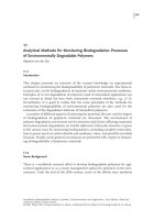
For small 𝜃, 𝑠𝑖𝑛𝜃 ≈ 𝜃 ⟹ 0.23 + 0.5𝑚𝐿2 𝜃 = 𝑇𝑚 − 4.9𝑚𝐿𝜃
0.68𝜃 + 14.7𝜃 = 0.5
0.5
⟹𝜃 𝑡 =
1 − 𝑐𝑜𝑠4.65𝑡 = 0.034(1 − 𝑐𝑜𝑠4.65𝑡)
14.7
HCM City Univ. of Technology, Faculty of Mechanical Engineering

System Dynamics

Solution Methods for Dynamic Models

§1.Differential Equations
5.Sumary of the trial solution method
Ordinary Differential Equation Solution form
𝑏

𝑥 𝑡 = + 𝐶𝑒 −𝑎𝑡

𝑥 + 𝑎𝑥 = 𝐵, 𝑎 ≠ 0
𝑥 + 𝑎𝑥 + 𝑏𝑥 = 𝑐, 𝑏 ≠ 0
𝑎2 > 4𝑏 real roots, distinct
𝑠1 ≠ 𝑠2
𝑎2 = 4𝑏 real roots, repeated
𝑠1 = 𝑠2
𝑎 = 0, 𝑏 > 0 imaginary roots

𝑎

𝑥 𝑡 = 𝐶1 𝑒 𝑠1 𝑡 + 𝐶2 𝑒 𝑠2 𝑡 +

𝑥 𝑡 = (𝐶1 + 𝑡𝐶2 )𝑒 𝑠1 𝑡 +

𝑐
𝑏

𝑐
𝑏

𝑥 𝑡 = 𝐶1 𝑠𝑖𝑛𝜔𝑡 + 𝐶2 𝑐𝑜𝑠𝜔𝑡 +

𝑐
𝑏

𝑠 = ±𝑗𝜔, 𝜔 = 𝑏
𝑐
𝑎 ≠ 0, 𝑎2 < 4𝑏 complex roots 𝑥 𝑡 = 𝑒𝜎𝑡 𝐶1𝑠𝑖𝑛𝜔𝑡 + 𝐶2𝑐𝑜𝑠𝜔𝑡 +
𝑏
𝑠 = 𝜎 ± 𝑗𝜔, 𝜎 = −𝑎/2
𝜔 = 4𝑏 − 𝑎2 /2
HCM City Univ. of Technology, Faculty of Mechanical Engineering

System Dynamics

Nguyen Tan Tien

3.17

Solution Methods for Dynamic Models

§2.Response Types and Stability

- The solution of 𝑥 + 𝑎𝑥 = 𝑏
𝑏
𝑏
𝑥 𝑡 =
+ 𝑥 0 − 𝑒 −𝑎𝑡
𝑎
𝑎

or
𝑥 𝑡 = 𝑥 0 𝑒 −𝑎𝑡 +

𝑏
1 − 𝑒 −𝑎𝑡
𝑎

Response
• Steady-state: the part of the response that remains with time
• Transient: the part of the response that disappears with time
• Free: the part of the response that depends on the initial conditions
• Forced: the part of the response due to the forcing function
𝑥 + 𝑎𝑥 = 𝐵, 𝑎 ≠ 0

𝑏

𝑥 𝑡 = 𝑎 + 𝐶𝑒 −𝑎𝑡

HCM City Univ. of Technology, Faculty of Mechanical Engineering

3.14

Solution Methods for Dynamic Models

§1.Differential Equations
- Example 3.1.6
Two Complex Roots
Use trial solution method to solve the following problem for
𝑡 ≥ 0: 𝑥 + 6𝑥 + 34𝑥 = 68, 𝑥 0 = 5, 𝑥 0 = 7
Solution
Subtituting 𝑥 𝑡 = 𝐶 + 𝐷𝑒 𝑠𝑡 into the ODE
𝑠 2 + 6𝑠 + 34 𝐷𝑒 𝑠𝑡 + 34𝐶 = 68
𝑠 2 + 6𝑠 + 34 = 0 ⟹ 𝑠 = −3 ± 5𝑗, 𝐶 = 2
34𝐶 = 68
Therefore
𝑥 𝑡 = 𝐶 + 𝐷1 𝑒 (−3+5𝑗)𝑡 + 𝐷2 𝑒 (−3−5𝑗)𝑡
⟹ 𝑥 𝑡 = 𝐶 + 𝑒 −3𝑡 (𝐷1 𝑒 5𝑗𝑡 + 𝐷2 𝑒 −5𝑗𝑡 )
⟹ 𝑥 𝑡 = 𝐶 + 𝑒 −3𝑡 (𝐵1 𝑐𝑜𝑠5𝑡 + 𝐵2 𝑠𝑖𝑛5𝑡)
⟹

With the initial conditions 𝑥 𝑡 = 2 + 𝑒 −3𝑡 3𝑐𝑜𝑠5𝑡 +

Nguyen Tan Tien

3.15

System Dynamics

HCM City Univ. of Technology, Faculty of Mechanical Engineering

System Dynamics

5

𝑠𝑖𝑛5𝑡

Nguyen Tan Tien

3.16

Solution Methods for Dynamic Models

§1.Differential Equations
6.Assessment of Solution Behavior
- The characteristic equation can be quickly identified from ODE
by replacing 𝑥 with 𝑠, 𝑥 with 𝑠 2 , and so forth
- Example
3𝑥 + 30𝑥 + 222𝑥 = 148
The characteristic equation
𝑠 2 + 10𝑠 + 74 = 0
⟹ 𝑠 − −5 − 7𝑗 𝑠 − −5 + 7𝑗 = 0
The solution in the form
2
𝑥 𝑡 = 𝑒 −5𝑡 𝐶1 𝑠𝑖𝑛7𝑡 + 𝐶2 𝑐𝑜𝑠7𝑡 +
3

𝑐

𝑎 ≠ 0, 𝑎2 < 4𝑏 : 𝑠 = 𝜎 ± 𝑗𝜔, 𝜎 = −𝑎/2, 𝜔 = 4𝑏 − 𝑎2/2

𝑥 𝑡 = 𝑒𝜎𝑡 𝐶1 𝑠𝑖𝑛𝜔𝑡 + 𝐶2 𝑐𝑜𝑠𝜔𝑡 + 𝑏

HCM City Univ. of Technology, Faculty of Mechanical Engineering

System Dynamics

Nguyen Tan Tien

3.18

Solution Methods for Dynamic Models

§2.Response Types and Stability
1.The time constant
The 1st order model
𝑥 + 𝑎𝑥 = 𝑏
1
⟹ 𝑥 + 𝑥 = 𝑏,
𝜏 ≡ 1/𝑎
𝜏
give the free response
𝑥 𝑡 = 𝑥 0 𝑒 −𝑎𝑡
𝑡

⟹ 𝑥 𝑡 = 𝑥(0)𝑒 − 𝜏
𝜏: time constant
• measure of the exponential decay curve
• estimate how long it will take for the transient response to
disappear
𝑥 + 𝑎𝑥 = 𝑏, 𝑎 ≠ 0

Nguyen Tan Tien

16

𝑏

𝑥 𝑡 = 𝑎 + 𝐶𝑒 −𝑎𝑡

HCM City Univ. of Technology, Faculty of Mechanical Engineering

Nguyen Tan Tien

3


8/25/2013

System Dynamics

3.19

Solution Methods for Dynamic Models

§2.Response Types and Stability

System Dynamics

3.20

Solution Methods for Dynamic Models

§2.Response Types and Stability
The time constant is useful also for analyzing the response
when the forcing function is a constant
The total response in terms of 𝜏 by substituting 𝑎 = 1/𝜏
𝑥𝑡 =

𝑏𝜏
steady state

𝑡

𝑡

+ 𝑥 0 − 𝑏𝜏 𝑒− 𝜏 = 𝑥𝑠𝑠 + [𝑥 0 − 𝑥𝑠𝑠]𝑒− 𝜏
transient state

The response approaches the constant value 𝑏𝜏 as 𝑡 → ∞
𝑥𝑠𝑠 = lim 𝑥(𝑡) = 𝑏𝜏
𝑡→∞

From figure
• after 𝑡 = 𝜏, 𝑥(𝑡) has decayed to 37% of its initial value
• after 𝑡 = 4𝜏, 𝑥(𝑡) has decayed to 02% of its initial value
HCM City Univ. of Technology, Faculty of Mechanical Engineering

System Dynamics

3.21

Nguyen Tan Tien

Solution Methods for Dynamic Models

§2.Response Types and Stability

System Dynamics

3.23

Nguyen Tan Tien

Solution Methods for Dynamic Models

§2.Response Types and Stability
2.The Dominant-Root Approximation
- The time constant concept is not limited to first-order models.
It can also be used to estimate the response time of higherorder models
- Example 3.2.2 Responses for Second-Order, Complex Roots
Identify the responses of the equation
𝑥 + 6𝑥 + 34𝑥 = 𝑐 (𝑠 = −3 ± 5𝑗)
Solution
Following the procedure used in Example 3.1.6
𝑐
𝑥 𝑡 =
+ 𝑒 −3𝑡 𝐵1 𝑐𝑜𝑠5𝑡 + 𝐵2 𝑠𝑖𝑛5𝑡
34

𝑥 + 𝑎𝑥 + 𝑏𝑥 = 𝑐,𝑎2 < 4𝑏:𝑠 = 𝜎 ± 𝑗𝜔,𝜎 = −𝑎/2,𝜔 = 4𝑏 − 𝑎2/2
HCM City Univ. of Technology, Faculty of Mechanical Engineering

System Dynamics

3.22

Nguyen Tan Tien

Solution Methods for Dynamic Models

§2.Response Types and Stability
- Example 3.2.1 Responses for Second-Order, Distinct Roots
Identify the responses of 𝑥 + 7𝑥 + 10𝑥 = 𝑐 (roots: −2, −5)
Solution
𝑐
The solution 𝑥 𝑡 =
+ 𝐷1𝑒 −2𝑡 + 𝐷2 𝑒 −5𝑡
10
Submit to ODE
5
1
𝑐
2
1
𝑐
⟹ 𝐷1 = 𝑥 0 + 𝑥 0 − , 𝐷2 = − 𝑥 0 − 𝑥 0 +
3
3
6
3
3
15

Arranging the solution in another form
5
1
2
1
𝑥 𝑡 = 𝑥 0 + 𝑥 0 𝑒 −2𝑡 + − 𝑥 0 − 𝑥 0 𝑒 −5𝑡
3
3
3
3
1 1 −2𝑡
+𝑐
− 𝑒
10 6

The forced response (for which 𝑥(0) = 0) is plotted in the figure
• at 𝑡 = 𝜏, the response is 63% of the steady-state value
• at 𝑡 = 4𝜏, the response is 98% of the steady-state value
• at 𝑡 = 5𝜏, the response is 99% of the steady-state value
For most engineering purposes: 𝑥(𝑡) reaches steady-state at 𝑡 = 4𝜏
HCM City Univ. of Technology, Faculty of Mechanical Engineering

HCM City Univ. of Technology, Faculty of Mechanical Engineering

HCM City Univ. of Technology, Faculty of Mechanical Engineering

System Dynamics

3.24

Nguyen Tan Tien

Solution Methods for Dynamic Models

§2.Response Types and Stability
The coefficients 𝐵1 and 𝐵2 can be found in terms of arbitrary
initial conditions in the usual way
𝑐
34𝑥 0 + 102𝑥 0 − 3𝑐
𝐵1 = 𝑥 0 − , 𝐵2 =
34
170
𝑥 0 + 3𝑥(0) −3𝑡
⟹ 𝑥 𝑡 = 𝑥 0 𝑒 −3𝑡 𝑐𝑜𝑠5𝑡 +
𝑒 𝑠𝑖𝑛5𝑡
5
+

𝑐
3
1 − 𝑒 −3𝑡 𝑐𝑜𝑠5𝑡 − 𝑒 −3𝑡 𝑠𝑖𝑛5𝑡
34
5

Model’s time constant: τ = 1/3 ⟹ the response is essentially
at steady state for 𝑡 > 4τ = 4/3

𝑐

𝑥 𝑡 = 𝑒𝜎𝑡 𝐶1𝑠𝑖𝑛𝜔𝑡 + 𝐶2𝑐𝑜𝑠𝜔𝑡 + 𝑏

Nguyen Tan Tien

HCM City Univ. of Technology, Faculty of Mechanical Engineering

Nguyen Tan Tien

4


8/25/2013

System Dynamics

3.25

Solution Methods for Dynamic Models

§2.Response Types and Stability
3.Time Constants and Complex Roots
- Example 3.2.3 Responses for Second-Order, Imaginary Roots
Identify the responses of 𝑥 + 16𝑥 = 𝑐
Solution
The characteristic roots 𝑠 = ±4𝑗, the solution form
𝑐
𝑥 𝑡 =
+ 𝐵1 𝑐𝑜𝑠4𝑡 + 𝐵2 𝑠𝑖𝑛4𝑡
16

no terms that disappear as 𝑡 → ∞ ⟹ no transient response
The free and forced responses

𝑥(0)
𝑐
𝑥 𝑡 = 𝑥 0 𝑐𝑜𝑠4𝑡 +
𝑠𝑖𝑛4𝑡 + (1 − 𝑐𝑜𝑠4𝑡)
4
16
𝑥 + 𝑎 𝑥 + 𝑏𝑥 = 𝑐: 𝑠 = ±𝑗𝜔, 𝜔 = 𝑏

𝑥 𝑡 = 𝐶1 𝑠𝑖𝑛𝜔𝑡 + 𝐶2 𝑐𝑜𝑠𝜔𝑡 +

HCM City Univ. of Technology, Faculty of Mechanical Engineering

System Dynamics

3.27

𝑐
𝑏

Nguyen Tan Tien

Solution Methods for Dynamic Models

§2.Response Types and Stability
- The stability properties of a linear model are determined from
its characteristics roots
- The first-order model
𝑥 + 𝑎𝑥 = 𝑓(𝑡)
The characteristic equation 𝑠 + 𝑎 = 0
The free response

𝑥 𝑡 = 𝑥(0)𝑒 −𝑎𝑡
𝑠 = −𝑎 < 0: 𝑡 ⟶ ∞, 𝑥(𝑡) ⟶ 0: the model is stable
𝑠 = −𝑎 > 0: 𝑡 ⟶ ∞, 𝑥(𝑡) ⟶ ∞ : the model is unstable
𝑠 = 𝑎 = 0: 𝑡 ⟶ ∞, 𝑥(𝑡) ↛ 0, ∞: the model is neural stability

System Dynamics

3.26

Solution Methods for Dynamic Models

§2.Response Types and Stability
4.Stability

- Unstable: the free response approaches ∞ as 𝑡 → ∞
- Stable: the free response approaches 0
- Neutral stability: the borderline between stable and unstable.
The free response does not approach both ∞ and 0
HCM City Univ. of Technology, Faculty of Mechanical Engineering

System Dynamics

3.28

Nguyen Tan Tien

Solution Methods for Dynamic Models

§2.Response Types and Stability
- The second-order models with the same initial conditions

𝑥 0 = 1; 𝑥 0 = 1
1. 𝑥 − 4𝑥 = 𝑓(𝑡)
𝑠 = ±2 + 0𝑗
1
𝑥 𝑡 = 𝑒 2𝑡 + 𝑒 −2𝑡
2
2. 𝑥 − 4𝑥 + 229𝑥 = 𝑓(𝑡)
𝑠 = +2 ± 15𝑗
2
𝑥 𝑡 = 𝑒2𝑡 𝑐𝑜𝑠15𝑡 − 𝑠𝑖𝑛15𝑡
15
3. 𝑥 + 256𝑥 = 𝑓(𝑡)
𝑠 = 0 ± 16𝑗
𝑥 𝑡 = 𝑐𝑜𝑠16𝑡

HCM City Univ. of Technology, Faculty of Mechanical Engineering

System Dynamics

3.29

Nguyen Tan Tien

Solution Methods for Dynamic Models

§2.Response Types and Stability
- Stability Test for Linear Constant-Coefficient Models
• A constant-coefficient linear model is stable if and only if all
of its characteristic roots have negative real parts
• The model is neutrally stable if one or more roots have a

zero real part, and the remaining roots have negative real
parts
• The model is unstable if any root has a positive real part

HCM City Univ. of Technology, Faculty of Mechanical Engineering

Nguyen Tan Tien

HCM City Univ. of Technology, Faculty of Mechanical Engineering

System Dynamics

3.30

Nguyen Tan Tien

Solution Methods for Dynamic Models

§2.Response Types and Stability
5.A Physical Example
- Pendulum motion equation (𝜃 ≈ 0)
𝑚𝐿2 𝜃 + 𝑐𝜃 + 𝑚𝑔𝐿𝜃 = 0
- Equilibrium point: 𝜃 = 0
−𝑐 ± 𝑐 2 − 4𝑚2 𝐿3 𝑔
2𝑚𝐿2
• 2𝑚𝐿 𝐿𝑔 > 𝑐 > 0: damped oscillating

Roots

𝑠=

• 𝑐 > 2𝑚𝐿 𝐿𝑔:

no oscillating

• 𝑐 = 0:

oscillating about 𝜃 = 0

HCM City Univ. of Technology, Faculty of Mechanical Engineering

Nguyen Tan Tien

5


8/25/2013

System Dynamics

3.31

Solution Methods for Dynamic Models

§2.Response Types and Stability
- Pendulum motion equation (𝜃 ≈ 0)
𝑚𝐿2 𝜃 + 𝑐𝜃 + 𝑚𝑔𝐿𝜃 = 0
- Equilibrium point: 𝜃 = 𝜋
−𝑐 ± 𝑐 2 + 4𝑚2 𝐿3 𝑔
2𝑚𝐿2

- Pendulum will not oscillate about 𝜃 = 𝜋 but will
continue to fall away if disturbed ⟹ the system
is unstable
- The model is based on the assumption that 𝜃 ≈
0 ⟹ cannot draw any conclusions from the
model regarding the behavior when 𝜃 is not
near 𝜋
𝑠=

Roots

HCM City Univ. of Technology, Faculty of Mechanical Engineering

System Dynamics

3.33

Nguyen Tan Tien

Fluid and Thermal Systems

System Dynamics

3.32

Solution Methods for Dynamic Models

§2.Response Types and Stability
6.Routh-Hurwitz Condition
- The characteristic equation of many systems has the form

𝑚𝑠 2 + 𝑐𝑠 + 𝑘 = 0
- Routh-Hurwitz condition: the second-order system whose
characteristic polynomial is 𝑚𝑠 2 + 𝑐𝑠 + 𝑘 = 0 is stable if and
only if 𝑚, 𝑐, and 𝑘 have the same sign

HCM City Univ. of Technology, Faculty of Mechanical Engineering

System Dynamics

3.34

Nguyen Tan Tien

Fluid and Thermal Systems

§2.Response Types and Stability
7.Stability and Equilibrium
- An equilibrium: a state of no change
The pendulum in the figure is in equilibrium at
𝜃 = 0 and when perfectly balanced at 𝜃 = 𝜋
• the equilibrium at 𝜃 = 0:
stable
• the equilibrium at 𝜃 = 𝜋: unstable
⟹ the same physical system can have different
stability characteristics at different equilibria
- Stability is not a property of the system alone, but is a
property of a specific equilibrium of the system
- When we speak of the stability properties of a model, we are
actually speaking of the stability properties of the specific
equilibrium on which the model is based

§2.Response Types and Stability
- The figure shows a ball on a surface that has a valley and a hill

HCM City Univ. of Technology, Faculty of Mechanical Engineering

HCM City Univ. of Technology, Faculty of Mechanical Engineering

System Dynamics

3.35

Nguyen Tan Tien

Fluid and Thermal Systems

§3.The Laplace Transform Method
- The Laplace transforms the problem in time-domain to
problem in s-domain, then applying the solution in s-domain,
and finally using inverse transform to converse the solution
back to the time-domain

- The bottom of the valley is an equilibrium, and if the ball is
displaced slightly from this position, it will
• oscillate forever about the bottom if there is no friction:
neutrally stable
• return to the bottom if friction is present: stable
- If displace the ball so much to the left that it lies outside the
valley, it will never return: locally stable but globally unstable
- If the system returns to its equilibrium for any initial

displacement: globally stable
- The equilibrium on the hilltop is globally unstable

System Dynamics

3.36

Nguyen Tan Tien

Fluid and Thermal Systems

§3.The Laplace Transform Method
- Notation for the Laplace and inverse Laplace transforms
𝑋 𝑠 =ℒ 𝑥 𝑡
𝑥 𝑡 = ℒ −1 {𝑋(𝑠)}
- Table of Laplace transform pairs

- The Laplace transform ℒ{𝑥 𝑡 } of a function 𝑥(𝑡) is defined as
𝑇

ℒ 𝑥 𝑡

𝑥 𝑡 𝑒 −𝑠𝑡 𝑑𝑡

= lim

𝑇→∞

0

but is usually expressed more compactly as
∞

ℒ 𝑥 𝑡

𝑥 𝑡 𝑒 −𝑠𝑡 𝑑𝑡

=
0

HCM City Univ. of Technology, Faculty of Mechanical Engineering

Nguyen Tan Tien

HCM City Univ. of Technology, Faculty of Mechanical Engineering

Nguyen Tan Tien

6


8/25/2013

System Dynamics

3.37

Fluid and Thermal Systems

§3.The Laplace Transform Method

System Dynamics

3.38

Fluid and Thermal Systems

§3.The Laplace Transform Method
1.Transforms of Common Functions
- Example 3.3.1
Transform of a Constant
Suppose 𝑥(𝑡) = 𝑐 , a constant, for 𝑡 ≥ 0 . Determine its
Laplace transform
Solution
From the transform definition
𝑇

𝑇

𝑐𝑒 −𝑠𝑡 𝑑𝑡 = 𝑐 lim

ℒ 𝑥(𝑡) = lim

𝑇→∞

0

1 −𝑠𝑡
𝑒
−𝑠

= 𝑐 lim

𝑇→∞

𝑒 −𝑠𝑡 𝑑𝑡

𝑇→∞

0

𝑇
0

1 −𝑠𝑇
1 −𝑠×0
𝑐
⟹ ℒ 𝑐 = 𝑐 lim
𝑒
−
𝑒
=
𝑇→∞ −𝑠
−𝑠
𝑠
HCM City Univ. of Technology, Faculty of Mechanical Engineering

System Dynamics

3.39

Nguyen Tan Tien

Fluid and Thermal Systems

§3.The Laplace Transform Method
- The step function

HCM City Univ. of Technology, Faculty of Mechanical Engineering

System Dynamics

3.40

𝑇

ℒ 𝑒 −𝑎𝑡 = lim

𝑇→∞

0 𝑡<0
𝑢𝑠 𝑡 =
1 𝑡>0

HCM City Univ. of Technology, Faculty of Mechanical Engineering

= lim

1
𝑒 − 𝑠+𝑎

−(𝑠 + 𝑎)

𝑇→∞

341

Nguyen Tan Tien

Fluid and Thermal Systems

§3.The Laplace Transform Method
2.Properties of the Laplace Transform

𝑒 −(𝑠+𝑎)𝑡 𝑑𝑡
0

𝑡
0
𝑇

− 𝑒 − 𝑠+𝑎

×0

1
𝑠+𝑎

HCM City Univ. of Technology, Faculty of Mechanical Engineering

System Dynamics

𝑇→∞
𝑇

1
𝑒 − 𝑠+𝑎
− 𝑠+𝑎

𝑇→∞

= 𝑀/𝑠

𝑇

𝑒 −𝑎𝑡 𝑒 −𝑠𝑡 𝑑𝑡 = lim
0

= lim

⟹ ℒ 𝑒 −𝑎𝑡 =

System Dynamics

Fluid and Thermal Systems

§3.The Laplace Transform Method
- Example 3.3.2
The Exponential Function
Derive the Laplace transform of the exponential function
𝑥(𝑡) = 𝑒 −𝑎𝑡 , where 𝑎 is a constant

Solution
From the transform definition

Unit-step function

Step function
𝑥(𝑡) = 𝑀𝑢𝑠 (𝑡)
𝑋 𝑠 = ℒ 𝑀𝑢𝑠 𝑡

Nguyen Tan Tien

3.42

Nguyen Tan Tien

Fluid and Thermal Systems

§3.The Laplace Transform Method
- Example 3.3.3
The Sine and Cosine Functions
Derive the Laplace transforms of 𝑒 −𝑎𝑡 𝑠𝑖𝑛𝜔𝑡 and 𝑒 −𝑎𝑡 𝑐𝑜𝑠𝜔𝑡,
where 𝑎 and 𝜔 are constants
Solution
Recall: - the Euler identity
𝑒𝑗𝜃 = 𝑐𝑜𝑠𝜃 + 𝑗𝑠𝑖𝑛𝜃, with 𝜃 = 𝜔𝑡
- the relation
1
𝑥 + 𝑗𝑦
𝑥 + 𝑗𝑦
=

=
𝑥 − 𝑗𝑦 (𝑥 − 𝑗𝑦)(𝑥 + 𝑗𝑦) 𝑥 2 + 𝑦 2
We have

𝑒 −𝑎𝑡 𝑐𝑜𝑠𝜔𝑡 + 𝑗𝑠𝑖𝑛𝜔𝑡 = 𝑒 −𝑎𝑡 𝑒𝑗𝜔𝑡 = 𝑒 − 𝑎−𝑗𝜔 𝑡
1
𝑠 + 𝑎 + 𝑗𝜔
ℒ 𝑒 −(𝑎−𝑗𝜔)𝑡 =
=
𝑠 + (𝑎 − 𝑗𝜔) (𝑠 + 𝑎)2 + (𝜔)2
HCM City Univ. of Technology, Faculty of Mechanical Engineering

Nguyen Tan Tien

HCM City Univ. of Technology, Faculty of Mechanical Engineering

(1)

Nguyen Tan Tien

7


8/25/2013

System Dynamics

3.43

Fluid and Thermal Systems

§3.The Laplace Transform Method
𝑠+𝑎
𝜔
ℒ 𝑒 −(𝑎−𝑗𝜔)𝑡 =
+𝑗
(𝑠 + 𝑎)2 +𝜔 2
(𝑠 + 𝑎)2 +𝜔 2
from eq.(1)
ℒ 𝑒 −(𝑎−𝑗𝜔)𝑡 = ℒ 𝑒 −𝑎𝑡 𝑐𝑜𝑠𝜔𝑡 + 𝑗𝑒 −𝑎𝑡 𝑠𝑖𝑛𝜔𝑡

System Dynamics

∞

Fluid and Thermal Systems

System Dynamics

3.47

∞

𝑡𝑥 𝑡 𝑒−𝑠𝑡𝑑𝑡
0

Nguyen Tan Tien

Fluid and Thermal Systems

§3.The Laplace Transform Method
b. From the time-shifting property

𝑥(𝑡)𝑒 −(𝑠+𝑎)𝑡 𝑑𝑡

=

0
−𝑎𝑡

⟹ ℒ 𝑒 𝑥(𝑡) = 𝑋(𝑠 + 𝑎)
where 𝑋 𝑠 = ℒ 𝑥(𝑡)
- Example 3.3.4
The Function 𝑡𝑒 −𝑎𝑡
Derive the Laplace transform of the function 𝑡𝑒 −𝑎𝑡
Solution
1
𝑥 𝑡 =𝑡⟹𝑋 𝑠 = 2
𝑠
1
1
ℒ 𝑡𝑒 −𝑎𝑡 = ℒ 𝑒 −𝑎𝑡 𝑥(𝑡) = 2
=
𝑠 𝑠→𝑠+𝑎 (𝑠 + 𝑎)2
HCM City Univ. of Technology, Faculty of Mechanical Engineering

System Dynamics

Nguyen Tan Tien

3.46

Fluid and Thermal Systems

𝑢𝑠 (𝑡 − 𝐷) is called the shifted step function. Determine 𝑋(𝑠)
Solution
𝑇
𝑇→∞

𝐷

𝑀𝑢𝑠(𝑡 − 𝐷)𝑒−𝑠𝑡𝑑𝑡 = lim

ℒ 𝑥(𝑡) = lim

𝑇→∞

0

𝑇

0 × 𝑒−𝑠𝑡𝑑𝑡 +
0

𝑀𝑒−𝑠𝑡𝑑𝑡
𝐷

𝑇

1 −𝑠𝑡

1 −𝑠𝑇
1 −𝑠𝐷
𝑒
= 𝑀 lim
𝑒
−
𝑒
𝑇→∞ −𝑠
−𝑠
−𝑠
𝐷
𝑀
⟹ ℒ 𝑥(𝑡) = 𝑒 −𝑠𝐷
𝑠
and ℒ 𝑢𝑠 (𝑡 −Faculty
𝐷) =
𝑒 −𝑠𝐷 /𝑠
HCM City Univ. of Technology,
of Mechanical Engineering
Nguyen Tan Tien
= 0 + 𝑀 lim

𝑇→∞

System Dynamics

3.48

Fluid and Thermal Systems

§3.The Laplace Transform Method
3.The Derivative Property
Applying integration by parts to the definition of the transform
∞
𝑑𝑥
𝑑𝑥 −𝑠𝑡
ℒ
=
𝑒 𝑑𝑡
𝑑𝑡
0 𝑑𝑡
= 𝑥 𝑡 𝑒 −𝑠𝑡

The pulse = A unit-step + A shifted, negative unit-step
𝑃(𝑡) = 𝑢𝑠 (𝑡) − 𝑢𝑠 (𝑡 − 𝐷)
From the time-shifting property
𝑃 𝑠 = ℒ 𝑢𝑠 𝑡 − ℒ 𝑢𝑠 𝑡 − 𝐷
1
1
= − 𝑒−𝑠𝐷
𝑠
𝑠
1
⟹ ℒ 𝑃 𝑡 = 1 − 𝑒 −𝑠𝐷
𝑠
HCM City Univ. of Technology, Faculty of Mechanical Engineering

𝑒 −𝑎𝑡 𝑥(𝑡)𝑒 −𝑠𝑡 𝑑𝑡
0

§3.The Laplace Transform Method
- Example 3.3.6
The Shifted Step Function
If the discontinuity in the unit-step function
occurs at 𝑡 = 𝐷
0 𝑡<𝐷
𝑥 𝑡 = 𝑀𝑢𝑠 (𝑡 − 𝐷) =
𝑀 𝑡>𝐷

- Example 3.3.5
The Function 𝑡𝑐𝑜𝑠𝜔𝑡
Derive the Laplace transform of the function 𝑡𝑐𝑜𝑠𝜔𝑡
Solution
𝑠
𝑥 𝑡 = 𝑐𝑜𝑠𝜔𝑡 ⟹ 𝑋 𝑠 = 2
𝑠 + 𝜔2
𝑑
𝑠
𝑠 2 − 𝜔2
ℒ 𝑡𝑐𝑜𝑠𝜔𝑡 = ℒ 𝑡𝑥(𝑡) = −
= 2
𝑑𝑠 𝑠 2 + 𝜔 2
𝑠 + 𝜔2 2
HCM City Univ. of Technology, Faculty of Mechanical Engineering

Fluid and Thermal Systems

∞

ℒ 𝑒 −𝑎𝑡 𝑥(𝑡) =

Nguyen Tan Tien

3.45

§3.The Laplace Transform Method
- Multiplication by 𝑡
∞
𝑑
𝑑
𝑋𝑠 =
𝑥 𝑡 𝑒−𝑠𝑡 𝑑𝑡 = −
𝑑𝑠
𝑑𝑠 0
= −ℒ{𝑡𝑥(𝑡)}
𝑑𝑋(𝑠)
⟹ ℒ 𝑡𝑥(𝑡) = −
𝑑𝑠

3.44

§3.The Laplace Transform Method
- Shifting along the 𝑠-axis or multiplication by an exponential

Comparing the above two equation, the Laplace transforms
of the exponentially decaying sine and cosine functions are
𝑠+𝑎
ℒ 𝑒 −𝑎𝑡 𝑐𝑜𝑠𝜔𝑡 =
(𝑠 + 𝑎)2 +𝜔 2
𝜔

ℒ 𝑒 −𝑎𝑡 𝑠𝑖𝑛𝜔𝑡 =
(𝑠 + 𝑎)2 +𝜔 2

HCM City Univ. of Technology, Faculty of Mechanical Engineering

System Dynamics

Nguyen Tan Tien

∞
0

∞

𝑥(𝑡)𝑒 −𝑠𝑡 𝑑𝑡

+𝑠
0

= 𝑠ℒ 𝑥 𝑡 − 𝑥 0
= 𝑠𝑋 𝑠 − 𝑥(0)
Extend to higher derivatives
𝑑2𝑥
ℒ
= 𝑠 2 𝑋 𝑠 − 𝑠𝑥 0 − 𝑥(0)
𝑑𝑡 2
ℒ

𝑑𝑛 𝑥
= 𝑠𝑛𝑋 𝑠 −

𝑑𝑡 𝑛

𝑛

𝑠 𝑛−𝑘 𝑔𝑘−1 ,
𝑘=1

HCM City Univ. of Technology, Faculty of Mechanical Engineering

𝑔𝑘−1 =

𝑑 𝑘−1 𝑥
𝑑𝑡𝑘−1

𝑡=0

Nguyen Tan Tien

8


8/25/2013

System Dynamics

3.49

Fluid and Thermal Systems

§3.The Laplace Transform Method

4.The Initial Value Theorem
Use to find the value of the function 𝑥(𝑡) at 𝑡 = 0+ (a time
infinitesimally greater than 0) with given the transform 𝑋(𝑠)
𝑥 0+ = lim 𝑥(𝑡) = lim [𝑠𝑋(𝑠)]
𝑡→0+

𝑠→∞

System Dynamics

HCM City Univ. of Technology, Faculty of Mechanical Engineering

System Dynamics

3.51

Nguyen Tan Tien

Fluid and Thermal Systems

§3.The Laplace Transform Method
6.Solving Equations with the Laplace Transform
Consider the linear first-order equation
𝑥 + 𝑎𝑥 = 𝑓(𝑡)
𝑓(𝑡): the input
𝑎: a constant
Multiply both sides of the equation by 𝑒 −𝑠𝑡 and then integrate
∞

∞

(𝑥 + 𝑎𝑥)𝑒 −𝑠𝑡 𝑑𝑡 =
0

𝑓(𝑡)𝑒 −𝑠𝑡 𝑑𝑡
0

ℒ 𝑥 + 𝑎𝑥 = ℒ{𝑓(𝑡)} ⟹ ℒ 𝑥 + 𝑎ℒ 𝑥 = ℒ{𝑓(𝑡)}
𝑠𝑋 𝑠 − 𝑥 0 + 𝑎𝑋 𝑠 = 𝐹 𝑠
𝑥(0)
1
⟹𝑋 𝑠 =
+
𝐹(𝑠)
𝑠+𝑎 𝑠+𝑎
𝑥(0)
1
⟹ 𝑥 𝑡 = ℒ −1
+ ℒ −1
𝐹(𝑠)
𝑠+𝑎
𝑠+𝑎

or
Then

free response

𝑡→∞

𝑠→0

𝑋 𝑠 =

7
(𝑠 + 4)2 +49

7𝑠
=0
+ 4)2 +49
This is confirmed by evaluating the inverse transform
𝑥 𝑡 = ℒ −1 𝑋 𝑠 = 𝑒 −4𝑡 sin7𝑡
⟹ 𝑥 ∞ = 𝑒 −(4×0) sin(7 × 0) = 0
The final value theorem does not apply to a periodic function
⟹ 𝑥 ∞ = lim 𝑠𝑋(𝑠) = lim
𝑠→0

𝑠→0 (𝑠

HCM City Univ. of Technology, Faculty of Mechanical Engineering

System Dynamics

3.52

Nguyen Tan Tien

Fluid and Thermal Systems

§3.The Laplace Transform Method

- Example 3.3.8
Step Response of a First-Order Equation
Suppose that the input 𝑓(𝑡) of the equation 𝑥 + 𝑎𝑥 = 𝑓(𝑡) is a
step function of magnitude 𝑀 whose transform is 𝐹(𝑠) = 𝑀/𝑠.
Obtain the expression for the complete response
Solution
The forced response is obtained from
1
1 𝑀
𝑀 1
1
𝑥 𝑡 = ℒ−1
𝐹(𝑠) = ℒ−1
= ℒ−1
−
𝑠 +𝑎
𝑠+𝑎 𝑠
𝑎 𝑠 𝑠+𝑎
𝑀
⟹𝑥 𝑡 =
1 − 𝑒 −𝑎𝑡
𝑎
The complete response
𝑀
𝑥 𝑡 = 𝑥 0 𝑒 −𝑎𝑡 +
1 − 𝑒 −𝑎𝑡
𝑎

forced response

HCM City Univ. of Technology, Faculty of Mechanical Engineering

System Dynamics

Fluid and Thermal Systems

Example

Example
7𝑠 + 2
𝑋 𝑠 =
𝑠(𝑠 + 6)
7𝑠 + 2
⟹ 𝑥 0+ = lim 𝑠
=7
𝑠→∞ 𝑠(𝑠 + 6)
This is confirmed by evaluating the inverse transform
1 20
𝑥 𝑡 = ℒ −1 𝑋 𝑠 = + 𝑒 −6𝑡
3 3
1 20
1 20
⟹ 𝑥 0 = + 𝑒 −6×0 = +
=7
3 3
3 3

3.50

§3.The Laplace Transform Method

5.The Final Value Theorem
Use to find the limit of the function 𝑥(𝑡) as 𝑡 → ∞
𝑓 ∞ = lim 𝑓(𝑡) = lim 𝑠𝐹(𝑠)

3.53

Nguyen Tan Tien

Fluid and Thermal Systems

HCM City Univ. of Technology, Faculty of Mechanical Engineering

System Dynamics

3.54

§3.The Laplace Transform Method
- Example 3.3.9
Ramp Response of a First-Order Equation
Determine the complete response of the following model,
which has a ramp input 𝑥 + 3𝑥 = 5𝑡, 𝑥 0 = 10
Solution
Applying the transform to the equation we obtain
5
𝑠𝑋 𝑠 − 𝑥 0 + 3𝑋 𝑠 = 2
𝑠
𝑥(0)
5
10
5

⟹𝑋 𝑠 =
+
=
+
𝑠 + 3 𝑠 2 (𝑠 + 3) 𝑠 + 3 𝑠 2 (𝑠 + 3)
Express the second term on the right as
5
𝐶1 𝐶2
𝐶3
𝐶1 𝑠 + 3 + 𝐶2𝑠 𝑠 + 3 + 𝐶3𝑠2
≡ + +
=
𝑠2(𝑠 + 3) 𝑠2 𝑠 𝑠 + 3
𝑠2(𝑠 + 3)
𝐶2 + 𝐶3 𝑠 2 + 𝐶1 + 3𝐶2 𝑠 + 3𝐶1
=
𝑠 2 (𝑠 + 3)

§3.The Laplace Transform Method
Comparing the numerators
𝐶2 + 𝐶3 = 0
𝐶1 = 5/3
𝐶1 + 3𝐶2 = 0 ⟹ 𝐶2 = −5/9
3𝐶1 = 5
𝐶3 = 5/9

HCM City Univ. of Technology, Faculty of Mechanical Engineering

HCM City Univ. of Technology, Faculty of Mechanical Engineering

Nguyen Tan Tien

Nguyen Tan Tien

Fluid and Thermal Systems

The forced response
5
5 5
𝐶1 𝑡 + 𝐶2 + 𝐶3 𝑒 −3𝑡 = 𝑡 − + 𝑒 −3𝑡
3
9 9
The complete response
5
5 5
𝑥 𝑡 = 10𝑒−3𝑡 + 𝑡 − + 𝑒−3𝑡
3
9 9
For 𝑡 > 4/3 , 𝑒 −3𝑡 < 0.02, → the
response is approximately given
by 𝑥(𝑡) = 5𝑡/3 − 5/9
Nguyen Tan Tien

9


8/25/2013

System Dynamics

3.55

Fluid and Thermal Systems

System Dynamics

3.56

Fluid and Thermal Systems

§3.The Laplace Transform Method
- Example 3.3.10
Transform Inversion for Complex Factors
Invert the following transform
8𝑠 + 13
𝑋 𝑠 = 2
𝑠 + 4𝑠 + 53
Solution
Express 𝑋(𝑠) as a sum of terms
8𝑠 + 13
𝑋𝑠 =
(𝑠 + 2)2+72
(𝑠 + 2)
3
7
=8
−
(𝑠 + 2)2+72 7 (𝑠 + 2)2+72
3
⟹ 𝑥 𝑡 = 8𝑒 −2𝑡 𝑐𝑜𝑠7𝑡 − 𝑒 −2𝑡 𝑠𝑖𝑛7𝑡

7

§3.The Laplace Transform Method
- Example 3.3.11 Step Response of a Second-Order Equation
Obtain the complete response of the following model

HCM City Univ. of Technology, Faculty of Mechanical Engineering

HCM City Univ. of Technology, Faculty of Mechanical Engineering

System Dynamics

3.57

Nguyen Tan Tien

Fluid and Thermal Systems

𝑥 + 4𝑥 + 53𝑥 = 15𝑢𝑠 𝑡 𝑥 0 = 8, 𝑥 0 = −19
Solution
Transforming the equation gives
𝑠2𝑋 𝑠 − 𝑠𝑥 0 − 𝑥 0 + 4 𝑠𝑋 𝑠 − 𝑥 0 + 53𝑋 𝑠 =

15
𝑠

Solve for 𝑋(𝑠) using the given initial conditions
𝑥 0 𝑠 + 𝑥 0 + 4𝑥(0)
15
𝑋 𝑠 =

+
𝑠 2 + 4𝑠 + 53
𝑠(𝑠 2 + 4𝑠 + 53)
8𝑠 + 13
15
(1)
= 2
+
𝑠 + 4𝑠 + 53 𝑠(𝑠 2 + 4𝑠 + 53)
The first term on the right of eq.(1) corresponds to the free
response 8𝑒 −2𝑡 𝑐𝑜𝑠7𝑡 − (3/7)𝑒 −2𝑡 𝑠𝑖𝑛7𝑡 (Ex. 3.3.10)
(2)

System Dynamics

3.58

Nguyen Tan Tien

Fluid and Thermal Systems

§3.The Laplace Transform Method
The second term on the right of eq.(1) corresponds to the
forced response. It can be expressed as follows
15
𝐶1
𝑠+2
7
= + 𝐶2
+ 𝐶3

𝑠[ 𝑠 + 2 2 + 72 ]
𝑠
𝑠 + 2 2 + 72
𝑠 + 2 2 + 72
𝐶1 𝑠 + 2 2 + 72 + 𝐶2 𝑠 𝑠 + 2 + 7𝐶3𝑠
=
𝑠[ 𝑠 + 2 2 + 72 ]
(𝐶1 + 𝐶2) 𝑠 + 2 2 + (4𝐶1 +2𝐶2 + 7𝐶3)𝑠 +53𝐶1
=
𝑠[ 𝑠 + 2 2 + 72 ]
Comparing numerators on the left and right sides
𝐶1 + 𝐶2 = 0
𝐶1 = 15/53
4𝐶1 + 2𝐶2 + 7𝐶3 = 0 ⟹ 𝐶2 = −15/53
53𝐶1 = 15
𝐶3 = −30/371
15 15 −2𝑡
30 −2𝑡
−
𝑒 𝑐𝑜𝑠7𝑡 −
𝑒 𝑠𝑖𝑛7𝑡 (3)
The forced response
53 53
371

§3.The Laplace Transform Method
The complete response is the sum of the free and forced
responses given by equations
15 409 −2𝑡
27 −2𝑡

𝑥 𝑡 =
−
𝑒 𝑐𝑜𝑠7𝑡 −
𝑒 𝑠𝑖𝑛7𝑡
(3)
53 53
371

HCM City Univ. of Technology, Faculty of Mechanical Engineering

HCM City Univ. of Technology, Faculty of Mechanical Engineering

System Dynamics

3.59

Nguyen Tan Tien

Fluid and Thermal Systems

The oscillations are difficult to see for 𝑡 > 2 because 𝑒−2𝑡 < 0.02
for 𝑡 > 2. So for most practical purposes we may say that the
response is essentially constant with a value 15/53 for 𝑡 > 2

System Dynamics

3.60

Nguyen Tan Tien

Fluid and Thermal Systems

§3.The Laplace Transform Method
Alternatively, combine the terms on the right side of eq.(1)
𝑥 0 𝑠 2 + 𝑥 0 + 4𝑥 0 𝑠 + 15 8𝑠 2 + 13𝑠 + 15
𝑋 𝑠 =
=
𝑠(𝑠 2 + 4𝑠 + 53)
𝑠[ 𝑠 + 2 2 + 72 ]
𝐶1
𝑠+2
7
= + 𝐶2
+ 𝐶3
𝑠
𝑠 + 2 2 + 72
𝑠 + 2 2 + 72
2
𝐶1 + 𝐶2 𝑠 + 4𝐶1 + 2𝐶2 + 7𝐶3 𝑠 + 53𝐶1
=
𝑠[ 𝑠 + 2 2 + 72 ]
Comparing numerators on the left and right sides
𝐶1 + 𝐶2 = 8
𝐶1 = 15/53
4𝐶1 + 2𝐶2 + 7𝐶3 = 13 ⟹ 𝐶2 = 409/53
53𝐶1 = 15
𝐶3 = −27/53
The complete response
15 409 −2𝑡
27 −2𝑡

𝑥 𝑡 =
−
𝑒 𝑐𝑜𝑠7𝑡 −
𝑒 𝑠𝑖𝑛7𝑡
53 53
371

§3.The Laplace Transform Method
Step response of a second-order equation with complex roots
Using a transform of the following form
𝐴𝑠2 + 𝐵𝑠 + 𝐶
1
𝑠+𝑎
𝑏
= 𝐶1 + 𝐶2
+ 𝐶3
𝑠[ 𝑠 + 𝑎 2 + 𝑏2]
𝑠
𝑠 + 𝑎 2 + 𝑏2
𝑠 + 𝑎 2 + 𝑏2
where the coefficients
𝐶
𝐵 − 𝑎𝐴 − 𝑎𝐶1
𝐶1 = 2
,
𝐶2 = 𝐴 − 𝐶1 ,
𝐶3 =
𝑎 + 𝑏2
𝑏
The response is

𝑥 𝑡 = 𝐶1 + 𝐶2 𝑒 −𝑎𝑡 𝑐𝑜𝑠𝑏𝑡 + 𝐶3 𝑒 −𝑎𝑡 𝑠𝑖𝑛𝑏𝑡

HCM City Univ. of Technology, Faculty of Mechanical Engineering

HCM City Univ. of Technology, Faculty of Mechanical Engineering

Nguyen Tan Tien

Nguyen Tan Tien

10


8/25/2013

System Dynamics

3.61

Fluid and Thermal Systems

System Dynamics

3.62

Fluid and Thermal Systems

§4.Transfer Function
- Response of a linear system = Free response + Forced response
• To focus the analysis on the effects of the input only by

taking the initial conditions to be zero temporarily
• Then, the free response due to any nonzero initial conditions
can be added to the result
- Consider the model 𝑥 + 𝑎𝑥 = 𝑓(𝑡)
Transforming both sides of the equation
𝑠𝑋 𝑠 + 𝑎𝑋 𝑠 = 𝐹 𝑠
obtain the transfer function
𝑋(𝑠)
1
𝑇 𝑠 =
=
𝐹(𝑠) 𝑠 + 𝑎
- A Transfer Function is the ratio of the output of a system to the
input of a system, in the Laplace domain considering its initial
conditions and equilibrium point to be zero

§4.Transfer Function
The TF concept is extremely useful for several reasons
- Transfer Functions and Software
• Matlab accepts a description based on the TF
• Simulink uses TF as the basis graphical system description
called the block diagram
- ODE Equivalence
The transfer function ⟺ The ODE
- The Transfer Function and Characteristic Roots
• The characteristic polynomial is the denominator of the TF
• The roots of characteristics equation give the information
about the stability of the system

HCM City Univ. of Technology, Faculty of Mechanical Engineering

HCM City Univ. of Technology, Faculty of Mechanical Engineering

System Dynamics

3.63

Nguyen Tan Tien

Fluid and Thermal Systems

System Dynamics

3.64

Nguyen Tan Tien

Fluid and Thermal Systems

§4.Transfer Function
- Example 3.4.1
Two Inputs and One Output
Obtain the transfer functions 𝑋(𝑠)/𝐹(𝑠) and 𝑋(𝑠)/𝐺(𝑠) for the
following equation
5𝑥 + 30𝑥 + 40𝑥 = 6𝑓 𝑡 − 20𝑔(𝑡)
Solution
Using the derivative property with zero initial conditions
5𝑠 2 𝑋 𝑠 + 30𝑠𝑋 𝑠 + 40𝑋 𝑠 = 6𝐹 𝑠 − 20𝐺(𝑠)
Solve for 𝑋(𝑠)
6

20
𝑋 𝑠 = 2
𝐹 𝑠 − 2
𝐺(𝑠)
5𝑠 + 30𝑠 + 40
5𝑠 + 30𝑠 + 40
The transfer function for a specific input can be obtained by
temporarily setting the other inputs equal to zero
𝑋(𝑠)
6
𝑋(𝑠)
20
=
,
=
𝐹(𝑠) 5𝑠 2 + 30𝑠 + 40
𝐺(𝑠) 5𝑠 2 + 30𝑠 + 40

§4.Transfer Function
- Example 3.4.2
A System of Equations
a.Obtain the transfer functions 𝑋(𝑠)/𝑉(𝑠) and 𝑌(𝑠)/𝑉(𝑠) of the
following system of equations
𝑥 = −3𝑥 + 2𝑦
𝑦 = −9𝑦 − 4𝑥 + 3𝑣(𝑡)
b.Obtain the forced response for 𝑥(𝑡) and 𝑦(𝑡) if the input is
𝑣(𝑡) = 5𝑢𝑠 (𝑡)

HCM City Univ. of Technology, Faculty of Mechanical Engineering

HCM City Univ. of Technology, Faculty of Mechanical Engineering

System Dynamics

3.65

Nguyen Tan Tien

Fluid and Thermal Systems

System Dynamics

3.66

§4.Transfer Function
Solution
a.Transform the system equations with zero initial conditions
𝑠𝑋 𝑠 = −3𝑋 𝑠 + 2𝑌 𝑠
𝑠𝑌 𝑠 = −9𝑌 𝑠 − 4𝑋 𝑠 + 3𝑉(𝑠)
𝑠+3
(1)
⟹𝑌 𝑠 =
𝑋(𝑠)
2
𝑠+3
𝑠+3
⟹𝑠
𝑋 𝑠 = −9
𝑋 𝑠 − 4𝑋 𝑠 + 3𝑉(𝑠)
2

2
Then solve for 𝑋(𝑠)/𝑉(𝑠) to obtain
𝑋(𝑠)
6
(2)
=
𝑉(𝑠) 𝑠 2 + 12𝑠 + 35
Now substitute eq.(2) into eq.(1) to obtain
𝑌(𝑠) 𝑠 + 2 𝑋(𝑠) 𝑠 + 3
6
3(𝑠 + 3)
=
=
=
(3)
𝑉(𝑠)
2 𝑉(𝑠)
2 𝑠2 + 12𝑠 + 35 𝑠2 + 12𝑠 + 35

§4.Transfer Function
b.From eq.(2)

HCM City Univ. of Technology, Faculty of Mechanical Engineering

HCM City Univ. of Technology, Faculty of Mechanical Engineering

Nguyen Tan Tien

Nguyen Tan Tien

Fluid and Thermal Systems

6
6
5
30
𝑉𝑠 = 2
=
𝑠2 + 12𝑠 + 35
𝑠 + 12𝑠 + 35 𝑠 𝑠(𝑠 + 5)(𝑠 + 7)
The partial-fraction expansion
𝐶1
𝐶2
𝐶3
𝑋 𝑠 = +
+
𝑠 𝑠+5 𝑠+7
where 𝐶1 = 6/7, 𝐶2 = −3, 𝐶3 = 15/7
The forced response
6
15
(4)
𝑥 𝑡 = − 3𝑒 −5𝑡 − 𝑒 −7𝑡
7
7
From eq.(1) 𝑦 = (𝑥 + 3𝑥)/2
From eq.(4), we obtain
9
30
𝑦 𝑡 = + 3𝑒 −5𝑡 − 𝑒 −7𝑡

7
7
𝑋𝑠 =

Nguyen Tan Tien

11


8/25/2013

System Dynamics

3.67

Fluid and Thermal Systems

System Dynamics

3.68

Fluid and Thermal Systems

§5.Partial Fraction Expansion
Use for the Inverse Laplace transform
Most transforms occur in the form of a ratio of two polynomials
𝑁(𝑠) 𝑏𝑚 𝑠 𝑚 + 𝑏𝑚−1 𝑠 𝑚−1 + ⋯ + 𝑏1 𝑠 + 𝑏0
𝑋 𝑠 =
=
𝐷(𝑠)

𝑠 𝑛 + 𝑎𝑛−1 𝑠 𝑛−1 + ⋯ + 𝑎1 𝑠 + 𝑎0
with 𝑚 ≤ 𝑛, the method of partial fraction expansion can be used
1.Distinct Root Case
If all the roots are distinct, 𝑋(𝑠) can be factored as follows
𝑁(𝑠)
𝑋𝑠 =
,
𝑠 = −𝑟1,−𝑟2, … , −𝑟𝑛
𝑠 + 𝑟1 𝑠 + 𝑟2 … (𝑠 + 𝑟𝑛)
𝐶1
𝐶2
𝐶𝑛
=
+
+⋯
,
𝐶𝑖 = lim [𝑋(𝑠)(𝑠 + 𝑟𝑖 )]
𝑠→−𝑟𝑖
𝑠 + 𝑟1 𝑠 + 𝑟2
𝑠 + 𝑟𝑛
Each factor corresponds to an exponential function of time
𝑥 𝑡 = 𝐶1 𝑒 −𝑟1 𝑡 + 𝐶2 𝑒 −𝑟2 𝑡 + ⋯ + 𝐶𝑛 𝑒 −𝑟𝑛 𝑡

§5.Partial Fraction Expansion
- Example 3.5.1
One Zero Root and One Negative Root
Obtain the inverse Laplace transform of
5
𝑋 𝑠 =
𝑠(𝑠 + 3)

Solution
The partial-fraction expansion has the form
5
𝐶1
𝐶2
𝑋 𝑠 =
= +
𝑠(𝑠 + 3)
𝑠 𝑠+3
Using the coefficient formula
5
5
5
𝐶1 = lim 𝑠
= lim
=
𝑠→0
𝑠→0 𝑠 + 3
𝑠 𝑠+3
3
5
5
5
𝐶2 = lim (𝑠 + 3)
= lim = −
𝑠→−3
𝑠→−3 𝑠
𝑠 𝑠+3
3
The inverse transform: 𝑥 𝑡 = 𝐶1 + 𝐶2 𝑒 −3𝑡 = (5/3) − (5/3)𝑒 −3𝑡

HCM City Univ. of Technology, Faculty of Mechanical Engineering

HCM City Univ. of Technology, Faculty of Mechanical Engineering

System Dynamics

3.69

Nguyen Tan Tien

Fluid and Thermal Systems

System Dynamics

3.70

Nguyen Tan Tien

Fluid and Thermal Systems

§5.Partial Fraction Expansion
- Example 3.5.2
A Third-Order Equation
Use two methods to obtain the solution of the following problem
𝑑3𝑥
𝑑2𝑥
𝑑𝑥
10 3 + 100 2 + 310 + 300𝑥 = 750𝑢𝑠 𝑡
𝑑𝑡

𝑑𝑡
𝑑𝑡
𝑥 0 = 2, 𝑥 0 = 4, 𝑥 0 = 3
Solution
a.Using the Laplace transform method
10 𝑠 3𝑋 𝑠 − 𝑥 0 − 𝑠𝑥 0 − 𝑠 2 𝑥 0
+100[𝑠 2𝑋 𝑠 − 𝑥 0 − 𝑠𝑥(0)]
750
+310 𝑠𝑋 𝑠 − 𝑥 0 + 300𝑋 𝑠 =
𝑠
Solving for 𝑋(𝑠) using the given initial values to obtain
2𝑠3 + 24𝑠2 + 105𝑠 + 75 2𝑠3 + 24𝑠2 + 105𝑠 + 75
𝑋𝑠 =
=
𝑠(𝑠3 + 10𝑠2 + 31𝑠 + 30)
𝑠(𝑠 + 2)(𝑠 + 3)(𝑠 + 5)

§5.Partial Fraction Expansion
The partial-fraction expansion
𝐶1
𝐶2
𝐶3
𝐶4
𝑋 𝑠 = +
+
+
𝑠 𝑠+2 𝑠+3 𝑠+5
The coefficients can be obtained from the formula
5
𝐶1 = lim 𝑠𝑋(𝑠) =

𝑠→0
2
55
𝐶2 = lim (𝑠 + 2)𝑋(𝑠) =
𝑠→−2
6
𝐶3 = lim (𝑠 + 3)𝑋(𝑠) = −13

HCM City Univ. of Technology, Faculty of Mechanical Engineering

HCM City Univ. of Technology, Faculty of Mechanical Engineering

System Dynamics

3.71

Nguyen Tan Tien

Fluid and Thermal Systems

§5.Partial Fraction Expansion

5 55 −2𝑡
10
+ 𝑒
− 13𝑒 −3𝑡 + 𝑒 −5𝑡
2 6
3
and 𝑒 −5𝑡 die out faster than 𝑒 −2𝑡

10
3

the answer is
5 55
10
𝑥 𝑡 = + 𝑒 −2𝑡 − 13𝑒 −3𝑡 + 𝑒 −5𝑡
2 6
3

System Dynamics

3.72

(1)
Nguyen Tan Tien

Fluid and Thermal Systems

𝑡→∞

5

• 𝑡 > 4/3: the response is approximately 𝑥 𝑡 = +
2

55 −2𝑡
𝑒
6

• 𝑡 > 2: the response is approximately constant at 𝑥 = 5/2
The “hump” in the response is produced by the positive
values of 𝑥(0) and 𝑥(0)
HCM City Univ. of Technology, Faculty of Mechanical Engineering

𝑠→−5

§5.Partial Fraction Expansion
b.The characteristic equation 10𝑠 3 + 100𝑠2 + 310𝑠 + 300 = 0,
which has the roots 𝑠 = −2, −3, −5 can be obtained from ODE
The characteristic equation roots generate the solution
𝑥 𝑡 = 𝐶1 + 𝐶2 𝑒 −2𝑡 + 𝐶3 𝑒 −3𝑡 + 𝐶4 𝑒 −5𝑡
(2)
The solution will approach zero as 𝑡 → ∞, leaving only a
constant term produced by the step input
𝐶1 = lim 𝑥(𝑡)

𝑥 𝑡 =
The terms 𝑒 −3𝑡

𝑠→−3

𝐶4 = lim (𝑠 + 5)𝑋(𝑠) =

Nguyen Tan Tien

𝐶1 can be found by setting the derivatives equal to zero in the
ODE and solving for 𝑥
10𝑥 + 100𝑥 + 310𝑥 + 300𝑥 = 750𝑢𝑠 𝑡
750 5

⟹ 𝐶1 = lim 𝑥(𝑡) =
=
𝑡→∞
300 2

HCM City Univ. of Technology, Faculty of Mechanical Engineering

Nguyen Tan Tien

12


8/25/2013

System Dynamics

3.73

Fluid and Thermal Systems

System Dynamics

3.74

Fluid and Thermal Systems

§5.Partial Fraction Expansion
The values of the remaining coefficients can be found with
the initial conditions by differentiating (2) to obtain
𝑥 0 = 𝐶1 + 𝐶2 + 𝐶3 + 𝐶4

5
= + 𝐶2 + 𝐶3 + 𝐶4
2
=2
𝑥 0 = −2𝐶2 − 3𝐶3 − 5𝐶4 = 4
𝑥 0 = 4𝐶2 + 9𝐶3 + 25𝐶4 = 3
The solution is 𝐶1 = 55/6, 𝐶2 = −13, and 𝐶3 = 10/3
And the answer is
5 55
10
𝑥 𝑡 = + 𝑒 −2𝑡 − 13𝑒 −3𝑡 + 𝑒 −5𝑡
2 6
3

§5.Partial Fraction Expansion
2.Repeated Root Case
Suppose that 𝑝 of the roots have the same value 𝑠 = −𝑟1, and
the remaining (𝑛 − 𝑝) roots are distinct and real. Then 𝑋(𝑠) is
of the form
𝑁(𝑠)
𝑋 𝑠 =
𝑠 + 𝑟1 𝑝 𝑠 + 𝑟𝑝+1 𝑠 + 𝑟𝑝+2 … (𝑠 + 𝑟𝑛 )

HCM City Univ. of Technology, Faculty of Mechanical Engineering

HCM City Univ. of Technology, Faculty of Mechanical Engineering

System Dynamics

3.75

Nguyen Tan Tien

Fluid and Thermal Systems

§5.Partial Fraction Expansion
The coefficients for the repeated roots are found from
𝐶1 = lim 𝑋 𝑠 𝑠 + 𝑟1 𝑝
𝑠→−𝑟1

𝐶2 = lim

𝑠→−𝑟1

𝑑
[𝑋 𝑠 𝑠 + 𝑟1 𝑝 ]
𝑑𝑠

⋮
𝐶𝑖 = lim

𝑠→−𝑟1

1
𝑑𝑖−1
[𝑋 𝑠 𝑠 + 𝑟1 𝑝 ] , 𝑖 = 1,2, … , 𝑝
𝑖 − 1 ! 𝑑𝑠 𝑖−1

The solution for the time function is
𝑡 𝑝−1 −𝑟 𝑡

𝑡 𝑝−2
𝑓 𝑡 = 𝐶1
𝑒 1 + 𝐶2
𝑒 −𝑟1 𝑡 + ⋯
𝑝−1 !
𝑝−2 !
+𝐶𝑝 𝑒 −𝑟1 𝑡 + ⋯ + 𝐶𝑝+1 𝑒 −𝑟𝑝+1 𝑡 + ⋯ + 𝐶𝑛 𝑒 −𝑟𝑛 𝑡

HCM City Univ. of Technology, Faculty of Mechanical Engineering

System Dynamics

3.77

Nguyen Tan Tien

Fluid and Thermal Systems

§5.Partial Fraction Expansion
5/3
𝐶2 + 𝐶3 𝑠 2 + 𝐶1 + 4𝐶2 𝑠 + 4𝐶1
=
2
𝑠 (𝑠 + 4)
𝑠 2 (𝑠 + 4)
Comparing numerators to obtain
𝐶2 + 𝐶3 = 0
𝐶1 = 5/12
𝐶1 + 4𝐶2 = 0 ⟹ 𝐶2 = −5/48
4𝐶1 = 5/3

𝐶3 = 5/48

𝑋 𝑠 =

System Dynamics

𝐶1
𝑠 + 𝑟1

𝑝

𝐶2
+⋯
𝑠 + 𝑟1 𝑝−1
𝐶𝑝
𝐶𝑝+1
𝐶𝑛
+
+ ⋯+
+⋯+
𝑠 + 𝑟1
𝑠 + 𝑟𝑝+1
𝑠 + 𝑟𝑛

+

3.76

Nguyen Tan Tien

Fluid and Thermal Systems

§5.Partial Fraction Expansion
- Example 3.5.3
One Negative Root and Two Zero Roots
Compare two methods for obtaining the inverse Laplace
transform of
5
𝑋 𝑠 = 2
𝑠 (3𝑠 + 12)
Solution
The partial-fraction expansion has the form
5
1
5
𝐶1 𝐶2
𝐶3
𝑋 𝑠 = 2
=
= + +
𝑠 (3𝑠 + 12) 3 𝑠 2 (𝑠 + 4) 𝑠 2 𝑠 𝑠 + 4
Using the coefficient formulas
5
5
5
𝐶1 = lim 𝑠 2 2
= lim
=
𝑠→0
𝑠→0 3(𝑠 + 4)

3𝑠 (𝑠 + 4)
12

HCM City Univ. of Technology, Faculty of Mechanical Engineering

System Dynamics

3.78

Nguyen Tan Tien

Fluid and Thermal Systems

§5.Partial Fraction Expansion
𝑑 2
5
𝑑
5
𝐶2 = lim
𝑠
= lim
𝑠→0 𝑑𝑠
𝑠→0 𝑑𝑠 3(𝑠 + 4)
3𝑠 2 (𝑠 + 4)
5
1
5
= lim −
=−
𝑠→0

3 (𝑠 + 4)2
48
5
5
5
𝐶3 = lim (𝑠 + 4) 2
= lim
=
𝑠→−4
𝑠→−4 3𝑠 2
3𝑠 (𝑠 + 4)
48

The inverse transform is
5
5
5
𝑡−
+ 𝑒 −4𝑡
12
48 48
For this example the two methods are roughly equivalent
• For repeated roots, coefficient formula requires that we
obtain the derivative of a ratio of functions
• The LCD method requires three equations to be solved
for three unknowns
𝑥 𝑡 = 𝐶1 𝑡 + 𝐶2 + 𝐶3 𝑒 −4𝑡 =

HCM City Univ. of Technology, Faculty of Mechanical Engineering

The expansion is

Nguyen Tan Tien

With the LCD (least common denominator) method we have
5/3
𝐶1 𝐶2
𝐶3
= + +
𝑠 2 (𝑠 + 4) 𝑠 2 𝑠 𝑠 + 4
𝐶1 𝑠 + 4 + 𝐶2 𝑠 𝑠 + 4 + 𝐶3 𝑠 2
=
𝑠 2 (𝑠 + 4)
𝐶1 + 𝐶3 𝑠 2 + 𝐶1 + 4𝐶2 𝑠 + 4𝐶1
=
𝑠 2 (𝑠 + 4)
HCM City Univ. of Technology, Faculty of Mechanical Engineering

Nguyen Tan Tien

13


8/25/2013

System Dynamics

3.79

Fluid and Thermal Systems

System Dynamics

3.80

Fluid and Thermal Systems

§5.Partial Fraction Expansion
- Example 3.5.4
Ramp Response of a First-Order Model
Use the Laplace transform to solve the following problem
3𝑥 + 12𝑥 = 5𝑡
𝑥 0 =0
Solution
Taking the transform of both sides of the equation
5
3 𝑠𝑋 𝑠 − 𝑥 0 + 12𝑋 𝑠 = 2
𝑠
Solve for 𝑋(𝑠) using the given value of 𝑥(0)
5
5 1
5 1 5 1
𝑋 𝑠 = 2
=
−
+
𝑠 (3𝑠 + 12) 12 𝑠 2 48 𝑠 48 𝑠 + 4
The inverse transform
5
5

5
𝑥 𝑡 =
𝑡−
+ 𝑒 −4𝑡
12
48 48

§5.Partial Fraction Expansion
- Example 3.5.5 Two Repeated Roots and One Distinct Root
Obtain the inverse Laplace transform of
7
𝑋 𝑠 =
𝑠 + 3 2 (𝑠 + 5)
Solution
The partial-fraction expansion has the form
7
𝐶1
𝐶2
𝐶3
𝑋 𝑠 =
=
+
+
𝑠 + 3 2 (𝑠 + 5)
𝑠+3 2 𝑠+3 𝑠+5
where
7
7
7
𝐶1 = lim 𝑠 + 3 2

= lim
=
𝑠→−3
𝑠→−3 𝑠 + 5
𝑠 + 3 2 (𝑠 + 5)
2

HCM City Univ. of Technology, Faculty of Mechanical Engineering

HCM City Univ. of Technology, Faculty of Mechanical Engineering

System Dynamics

3.81

Nguyen Tan Tien

Fluid and Thermal Systems

§5.Partial Fraction Expansion
7
7
7
= lim
=
𝑠→−3 𝑠 + 5
𝑠 + 3 2 (𝑠 + 5)
2
𝑑
7

𝑑
7
2
𝐶2 = lim
𝑠+3
= lim
𝑠→−3 𝑑𝑠
𝑠→−3 𝑑𝑠 𝑠 + 5
𝑠 + 3 2 (𝑠 + 5)
−7
7
= lim
=−
𝑠→−3 (𝑠 + 5)2
4
7
7
7
𝐶3 = lim 𝑠 + 5
= lim
=
𝑠→−5
𝑠→−5 (𝑠 + 3)2
𝑠 + 3 2 (𝑠 + 5)
4
𝐶1 = lim

𝑠→−3

𝑠+3

2

The inverse transform
𝑥 𝑡 = 𝐶1 𝑡𝑒 −3𝑡 + 𝐶2 𝑒 −3𝑡 + 𝐶3 𝑒 −5𝑡
7
7
7
= 𝑡𝑒 −3𝑡 − 𝑒 −3𝑡 + 𝑒 −5𝑡
2
4
4

HCM City Univ. of Technology, Faculty of Mechanical Engineering

System Dynamics

3.83

Nguyen Tan Tien

Fluid and Thermal Systems

§5.Partial Fraction Expansion
7
7
7
𝑥 𝑡 = 𝑡𝑒 −3𝑡 − 𝑒 −3𝑡 + 𝑒 −5𝑡
2
4

4

The “hump” in the response is caused by the multiplicative
factor of 𝑡 in the input (7/2)𝑡𝑒 −3𝑡
HCM City Univ. of Technology, Faculty of Mechanical Engineering

Nguyen Tan Tien

System Dynamics

3.82

Nguyen Tan Tien

Fluid and Thermal Systems

§5.Partial Fraction Expansion
- Example 3.5.6 Exponential Response of a First-Order Model
Use the Laplace transform to solve the following problem
𝑥 + 5𝑥 = 7𝑡𝑒 −3𝑡 ,
𝑥 0 =0
Solution
Taking the transform of both sides of the equation
7
𝑠𝑋 𝑠 − 𝑥 0 + 5𝑋 𝑠 =
(𝑠 + 3)2
Solve for 𝑋(𝑠) using the given value of 𝑥(0)
7
7
7

7
𝑋 𝑠 =
=
−
+
(𝑠 + 3)2 (𝑠 + 5) 2(𝑠 + 3)2 4 𝑠 + 3
4(𝑠 + 5)
The inverse transform
7
7
7
𝑥 𝑡 = 𝑡𝑒 −3𝑡 − 𝑒 −3𝑡 + 𝑒 −5𝑡
2
4
4
HCM City Univ. of Technology, Faculty of Mechanical Engineering

System Dynamics

3.84

Nguyen Tan Tien

Fluid and Thermal Systems

§5.Partial Fraction Expansion
- Example 3.5.7
Four Repeated Roots
Choose the most convenient method for obtaining the
inverse transform of

𝑠2 + 2
𝑋 𝑠 = 4
𝑠 (𝑠 + 1)
Solution
There are four repeated roots (𝑠 = 0) and one distinct root,
so the expansion is
𝐶1 𝐶2 𝐶3 𝐶4
𝐶5
𝑋 𝑠 = 4+ 3+ 2+ +
𝑠
𝑠
𝑠
𝑠 𝑠+1
There are four repeated roots, to find the coefficients would
require taking the first, second, and third derivatives of the
ratio (𝑠 2 + 2)/(𝑠 + 1). Therefore the LCD method is easier
to use for this problem
HCM City Univ. of Technology, Faculty of Mechanical Engineering

Nguyen Tan Tien

14


8/25/2013

System Dynamics

3.85

Fluid and Thermal Systems

System Dynamics

3.86

Fluid and Thermal Systems

§5.Partial Fraction Expansion
Using the LCD to obtain
𝐶1 𝑠 + 1 + 𝐶2𝑠 𝑠 + 1 + 𝐶3𝑠2 𝑠 + 1 + 𝐶4𝑠3 𝑠 + 1 + 𝐶5𝑠4
𝑋 𝑠 =
𝑠4(𝑠 + 1)
𝐶5 + 𝐶4 𝑠4 + 𝐶4 + 𝐶3 𝑠3 + 𝐶3 + 𝐶2 𝑠2 + 𝐶2 + 𝐶1 𝑠 + 𝐶1
=
𝑠4(𝑠 + 1)
Comparing numerators
𝑠2 + 2 = 𝐶5 + 𝐶4 𝑠4 + 𝐶4 + 𝐶3 𝑠3 + 𝐶3 + 𝐶2 𝑠2 + 𝐶2 + 𝐶1 𝑠 + 𝐶1
⟹ 𝐶1 = 2, 𝐶2 + 𝐶1 = 0, 𝐶3 + 𝐶2 = 1, 𝐶4 + 𝐶3 = 0, 𝐶5 + 𝐶4 = 0
⟹ 𝐶1 = 2, 𝐶2 = −2, 𝐶3 = 3, 𝐶4 = −3, 𝐶5 = 3
So the expansion
2
2
3 3
3
𝑋 𝑠 = 4− 3+ 2− +
𝑠
𝑠
𝑠
𝑠 𝑠+1

1
⟹ 𝑥 𝑡 = 𝑡 3 − 𝑡 2 + 3𝑡 − 3 + 3𝑒 −𝑡
3

§5.Partial Fraction Expansion
3.Complex Root
- Example 3.5.8
Two Complex Roots
Use two methods to obtain the inverse Laplace transform of
𝑋 𝑠 = (3𝑠 + 7)/(4𝑠 2 + 24𝑠 + 136)
Solution
a.Rewrite the equation in the form
3𝑠 + 7
1 3𝑠 + 7
𝑋𝑠 = 2
=
4𝑠 + 24𝑠 + 136 4 (𝑠 + 3)2+52
1
5
𝑠+3
1 𝐶2𝑠 + (5𝐶1 + 3𝐶2)
= 𝐶1
+ 𝐶2
=
4
(𝑠 + 3)2+52
(𝑠 + 3)2+52
4 (𝑠 + 3)2+52

HCM City Univ. of Technology, Faculty of Mechanical Engineering

HCM City Univ. of Technology, Faculty of Mechanical Engineering

System Dynamics

3.87

Nguyen Tan Tien

Fluid and Thermal Systems

Comparing the numerators to obtain 𝐶1 = −2/5, 𝐶2 = 3
The inverse transform is
1
1
1
3
𝑥 𝑡 = 𝐶1𝑒−3𝑡𝑠𝑖𝑛5𝑡 + 𝐶2𝑒−3𝑡𝑐𝑜𝑠5𝑡 = − 𝑒−3𝑡𝑠𝑖𝑛5𝑡 + 𝑒−3𝑡𝑐𝑜𝑠5𝑡
4
4
10
4

System Dynamics

3.88

Nguyen Tan Tien

Fluid and Thermal Systems

§5.Partial Fraction Expansion
b.The denominator roots are distinct and the expansion gives
3𝑠+7
3𝑠+7
𝐶1
𝐶2
𝑋𝑠 = 2
=
=
+
4𝑠 +24𝑠+136 4(𝑠+3−5𝑗)(𝑠+3+5𝑗) 𝑠+3−5𝑗 𝑠+3+5𝑗
3𝑠+ 7
−2+ 15𝑗 15+2𝑗
𝐶1 = lim (𝑠 +3− 5𝑗)𝑋(𝑠) = lim
=
=
𝑠→−3+5𝑗
𝑠→−3+5𝑗 4(𝑠+ 3+5𝑗)
40𝑗
40
This can be expressed in complex exponential form as follows
15 + 2𝑗 𝑗𝜙
229 𝑗𝜙
2
𝐶1 = 𝐶1 𝑒𝑗𝜙 =
𝑒 =
𝑒 ,𝜙 = 𝑡𝑎𝑛−1
= 0.1326𝑟𝑎𝑑
40

40
15
3𝑠 + 7
2 + 15𝑗 15− 2𝑗
𝐶2 = lim (𝑠 + 3 + 5𝑗)𝑋(𝑠) = lim
=
=
𝑠→−3−5𝑗
𝑠→−3−5𝑗 4(𝑠 + 3 − 5𝑗)
40𝑗
40
Note that 𝐶1 and 𝐶2 are complex conjugates. This will always
be the case for coefficients of complex-conjugate roots in a
partial-fraction expansion. Thus
𝐶2 = 𝐶1 𝑒 −𝑗𝜙 = 229𝑒 −0.1326𝑗 /40

§5.Partial Fraction Expansion
The inverse transform gives
𝑥 𝑡 = 𝐶1 𝑒 (−3+5𝑗)𝑡 + 𝐶2 𝑒 (−3−5𝑗)𝑡
= 𝐶1 𝑒 −3𝑡 𝑒 5𝑗𝑡 + 𝐶2 𝑒 −3𝑡 𝑒 −5𝑗𝑡
= 𝐶1 𝑒 −3𝑡 𝑒 5𝑡+𝜙 𝑗 + 𝑒 − 5𝑡+𝜙 𝑗
= 2 𝐶1 𝑒 −3𝑡 𝑐𝑜𝑠(5𝑡 + 𝜙)
where we have used the relation 𝑒𝑗𝜃 + 𝑒 −𝑗𝜃 = 2𝑐𝑜𝑠𝜃, which
can be derived from the Euler identity
Thus
229 −3𝑡
𝑥 𝑡 =
𝑒 𝑐𝑜𝑠(5𝑡 + 0.1326)
20
This answer is equivalent to that found in part (a), as can be

seen by applying the trigonometric identity
cos 5𝑡 + 𝜙 = 𝑐𝑜𝑠5𝑡𝑐𝑜𝑠𝜙 − 𝑠𝑖𝑛5𝑡𝑠𝑖𝑛𝜙

HCM City Univ. of Technology, Faculty of Mechanical Engineering

HCM City Univ. of Technology, Faculty of Mechanical Engineering

System Dynamics

3.89

Nguyen Tan Tien

Fluid and Thermal Systems

System Dynamics

3.90

Nguyen Tan Tien

Fluid and Thermal Systems

§5.Partial Fraction Expansion
- Example 3.5.9 Free Response of a 2nd-Order Model with Complex Roots
Use the Laplace transform to solve the following problem
7
35
4𝑥 + 24𝑥 + 136𝑥 = 0,
𝑥 0 = ,𝑥 0 = −

4
4
Solution
Taking the transform of both sides of the equation, we obtain
4 𝑠2𝑋 𝑠 − 𝑥 0 𝑠 − 𝑥 0 + 24 𝑠𝑋 𝑠 − 𝑥 0 + 136𝑋 𝑠 = 0
Solve for 𝑋(𝑠) using the given values of 𝑥(0) and 𝑥(0)
4 𝑥 0 𝑠 + 𝑥 0 + 24𝑥(0)
3𝑠 + 7
𝑋 𝑠 =
=
4𝑠 2 + 24𝑠 + 136
4(𝑠 2 + 6𝑠 + 34)
1
5
3
𝑠+3
=−
+
10 𝑠 + 3 2 + 52
4 (𝑠 + 3)2 +52
1
3
⟹ 𝑓 𝑡 = − 𝑒 −3𝑡 𝑠𝑖𝑛5𝑡 + 𝑒 −3𝑡 𝑐𝑜𝑠5𝑡
10
4

§6.The Impulse and Numerator Dynamics
- The effects of any inputs starting at 𝑡 = 0 are not felt by the
system until an infinitesimal time later, at 𝑡 = 0+
- The dependent variable 𝑥(𝑡) and its derivatives do not change

between 𝑡 = 0 and 𝑡 = 0+, and thus the solution 𝑥(𝑡) obtained
from the ODE will match the given initial conditions when 𝑥(𝑡)
and its derivatives are evaluated at 𝑡 = 0
- However, we will now investigate the behavior of some
systems for which 𝑥(0) = 𝑥(0+), or 𝑥(0) = 𝑥(0+), and so forth
for higher derivatives
- The initial value theorem gives the value at 𝑡 = 0+, which for
some models is not necessarily equal to the value at 𝑡 = 0. In
these cases the solution of the differential equation is correct
only for 𝑡 > 0. This phenomenon occurs in models having
impulse inputs and in models containing derivatives of a
discontinuous input, such as a step function

HCM City Univ. of Technology, Faculty of Mechanical Engineering

HCM City Univ. of Technology, Faculty of Mechanical Engineering

Nguyen Tan Tien

Nguyen Tan Tien

15


8/25/2013

System Dynamics

3.91

Fluid and Thermal Systems

System Dynamics

3.92

Fluid and Thermal Systems

§6.The Impulse and Numerator Dynamics
1.The Impulse
- Impulse: an input that is suddenly applied
and removed after a very short time
- Rectangular pulse: a constant input that is
suddenly removed
• its transform is 𝑀(1 − 𝑒 −𝑠𝐷 )/𝑠
• the strength of the pulse ≡ area under the pulse 𝐴 = 𝑀𝐷
If 𝐴 = 𝑐𝑜𝑛𝑠𝑡𝑎𝑛𝑡 and 𝐷 ⟶ 0: we obtain the impulse
- The transform 𝐹(𝑠) of an impulse
1 − 𝑒−𝑠𝐷
𝐴 1 − 𝑒−𝑠𝐷
𝐴𝑠𝑒−𝑠𝐷
𝐹 𝑠 = lim 𝑀
= lim
= lim
=𝐴
𝐷→0
𝐷→0 𝐷
𝐷→0
𝑠
𝑠

𝑠
If 𝐴 = 1: unit impulse or Dirac delta function 𝛿(𝑡)
- Consider the impulse 𝛿(𝑡) to start at time 𝑡 = 0 and finish at
𝑡 = 0+, with its effects first felt at 𝑡 = 0+

§6.The Impulse and Numerator Dynamics
- Example 3.6.1
Impulse Response of a Simple First-Order Model
Obtain the unit-impulse response of the model 𝑥 = 𝛿(𝑡)
a. by separation of variables
b. with the Laplace transform
The initial condition is 𝑥(0) = 3 , what is the value of 𝑥(0+) ?
Solution
a. Integrate both sides of the equation 𝑥 = 𝛿(𝑡) to obtain

HCM City Univ. of Technology, Faculty of Mechanical Engineering

HCM City Univ. of Technology, Faculty of Mechanical Engineering

System Dynamics

3.93

Nguyen Tan Tien

Fluid and Thermal Systems

𝑥(𝑡)

𝑡

𝑥 𝑡 𝑑𝑥 =
𝑥(0)

𝛿 𝑡 𝑑𝑡
0

or
𝑥 𝑡 −𝑥 0 =1⟹𝑥 𝑡 =𝑥 0 +1=3+1=4
This is the solution for 𝑡 > 0 but not for 𝑡 = 0
Thus, 𝑥 0+ = 4 but 𝑥 0 = 3, so the impulse has changed
𝑥(𝑡) instantaneously from 3 to 4

System Dynamics

3.94

Nguyen Tan Tien

Fluid and Thermal Systems

§6.The Impulse and Numerator Dynamics
b. The transformed equation is
𝑠𝑋 𝑠 − 𝑥 0 = 1
or
1 + 𝑥(0)
𝑋 𝑠 =
𝑠
which give the solution
−1

𝑥 𝑡 = ℒ 𝑋 𝑠 = [1 + 𝑥 0 ] × 1 = 4
Note that the initial value used with the derivative property is
the value of 𝑥 at 𝑡 = 0
The initial value theorem gives
1 + 𝑥(0)
𝑥 0+ = lim 𝑠𝑋(𝑠) = lim 𝑠
=1+3 =4
𝑠→∞
𝑠→∞
𝑠
which is correct

§6.The Impulse and Numerator Dynamics
- Example 3.6.2
Impulse Response of a First-Order Model
Obtain the unit-impulse response of the following model
𝑋(𝑠)/𝐹(𝑠) = 1/(𝑠 + 5)
The initial condition is 𝑥(0) = 0. What is the value of 𝑥(0+) ?
Solution
Because 𝑓(𝑡) = 𝛿(𝑡), 𝐹(𝑠) = 1, and the response is obtained from
1
1
𝑋 𝑠 =
𝐹 𝑠 =
𝑠+5
𝑠+5
The response is 𝑥(𝑡) = 𝑒 −5𝑡 for 𝑡 > 0. This gives
𝑥 0+ = lim 𝑥(𝑡) = lim 𝑒 −5𝑡 = 1

HCM City Univ. of Technology, Faculty of Mechanical Engineering

HCM City Univ. of Technology, Faculty of Mechanical Engineering

𝑡→0+

𝑠→∞

System Dynamics

3.95

Nguyen Tan Tien

Fluid and Thermal Systems

𝑡→0+

the impulse input has changed 𝑥 from 𝑥 0 = 0 to 𝑥(0+) = 1
This same result can be obtained from the initial value theorem
𝑥 0+ = lim 𝑠𝑋(𝑠) = lim [𝑠/(𝑠 + 5)] = 1

System Dynamics

𝑠→∞

3.96

Nguyen Tan Tien

Fluid and Thermal Systems

§6.The Impulse and Numerator Dynamics
- Example 3.6.3 Impulse Response of a Simple Second-Order Model
Obtain the unit-impulse response of the model 𝑥 = 𝛿(𝑡)
a. by separation of variables
b. with the Laplace transform
The initial condition is 𝑥(0) = 5 and 𝑥 0 = 10, what is the
value of 𝑥(0+) and 𝑥(0+) ?
Solution
a. Let 𝑣(𝑡) ≡ 𝑥(𝑡) ⟶ 𝑣 = 𝛿(𝑡) . Integrate 𝑣 = 𝛿(𝑡) to obtain
𝑣(𝑡) = 𝑣(0) + 1 = 10 + 1 = 11. Thus 𝑥 0+ = 11 ≠ 𝑥(0)
Now integrate 𝑥 = 𝑣 = 11 to obtain 𝑥(𝑡) = 𝑥(0) + 11𝑡 = 5 +
11𝑡. Thus, 𝑥 0+ = 5 = 𝑥(0)
So for this model the unit-impulse input changes 𝑥 from 𝑡 = 0
to 𝑡 = 0+ but does not change 𝑥

§6.The Impulse and Numerator Dynamics
b. The transformed equation is
𝑠 2 𝑋 𝑠 − 𝑠𝑥 0 − 𝑥 0 = 1
𝑠𝑥 0 + 𝑥 0 + 1 5𝑠 + 11 5 11
⟹𝑋 𝑠 =
=
= + 2
𝑠2
𝑠2
𝑠 𝑠
⟹ 𝑥 𝑡 = ℒ −1 {𝑋 𝑠 } = 5 + 11𝑡 and 𝑥 𝑡 = 11
Note that the initial values used with the derivative property
are the values at 𝑡 = 0
The initial value theorem gives

5𝑠 + 11
𝑥 0+ = lim 𝑠𝑋(𝑠) = lim 𝑠
=5
𝑠→∞
𝑠→∞
𝑠2
and because ℒ 𝑥 = 𝑠𝑋 𝑠 − 𝑥(0)
5𝑠 + 11
𝑥 0+ = lim 𝑠[𝑠𝑋 𝑠 − 𝑥 0 ] = lim 𝑠
− 5 = 11
𝑠→∞
𝑠→∞
𝑠2

HCM City Univ. of Technology, Faculty of Mechanical Engineering

HCM City Univ. of Technology, Faculty of Mechanical Engineering

Nguyen Tan Tien

as we found in part (a)
Nguyen Tan Tien

16


8/25/2013

System Dynamics

3.97

Fluid and Thermal Systems

System Dynamics

3.98

Fluid and Thermal Systems

§6.The Impulse and Numerator Dynamics
- Example 3.6.4
Impulse Response of a Second-Order Model
Obtain the unit-impulse response of the following model. The
initial conditions are 𝑥(0) = 0, 𝑥(0) = 0. What are the values of
𝑥(0+) and 𝑥(0+) ?
𝑋(𝑠)
1
=
𝐹(𝑠) 2𝑠 2 + 14𝑠 + 20
Solution
Because 𝐹(𝑠) = 1, the response is obtained from
1
𝑋 𝑠 = 2
𝐹 𝑠
2𝑠 + 14𝑠 + 20
1
1 1
1 1
= 2

=
−
2𝑠 + 14𝑠 + 20 6 𝑠 + 2 6 𝑠 + 5
and the response is
𝑥 𝑡 = (𝑒 −2𝑡 − 𝑒 −5𝑡 )/6

§6.The Impulse and Numerator Dynamics
This gives
𝑒 −2𝑡 − 𝑒 −5𝑡
𝑥 0+ = lim 𝑥 𝑡 = lim
=0
𝑡→0+
𝑡→0+
6
−2𝑒 −2𝑡 + 5𝑒 −5𝑡
1
𝑥 0+ = lim 𝑥(𝑡) = lim
=
𝑡→0+
𝑡→0+
6
2

HCM City Univ. of Technology, Faculty of Mechanical Engineering

HCM City Univ. of Technology, Faculty of Mechanical Engineering

System Dynamics

3.99

Nguyen Tan Tien

Fluid and Thermal Systems

So the impulse input has not changed 𝑥 between 𝑡 = 0 and 𝑡 =
0+ but has changed 𝑥 from 0 to 1/2
These results could have been obtained from the initial value
theorem
1
𝑥 0+ = lim 𝑠𝑋(𝑠) = lim 𝑠 2
=0
𝑠→∞
𝑠→∞ 2𝑠 + 14𝑠 + 20
1
1
𝑥 0+ = lim 𝑠[𝑠𝑋 𝑠 − 𝑥(0)] = lim 𝑠 2
=
𝑠→∞
𝑠→∞ 2𝑠 + 14𝑠 + 20
2

System Dynamics

3.100

Nguyen Tan Tien

Fluid and Thermal Systems

§6.The Impulse and Numerator Dynamics
In summary, be aware that the solution 𝑥(𝑡) and its derivatives
𝑥(𝑡), 𝑥(𝑡), … will match the given initial conditions at 𝑡 = 0 only if
there are no impulse inputs and no derivatives of inputs that are
discontinuous at 𝑡 = 0
If 𝑋(𝑠) is a rational function
• if the degree of the numerator of 𝑋(𝑠) is less than the degree
of the denominator, then the initial value theorem will give a
finite value for 𝑥(0+)
• if the degrees are equal, then initial value is undefined and the
initial value theorem is invalid, 𝑥(0+) is undefined
The latter situation corresponds to an impulse in 𝑥(𝑡) at 𝑡 = 0
and therefore 𝑥(0+) is undefined. For example, consider the
9𝑠 + 4
23
𝑋 𝑠 =
=9−
⟹ 𝑥 𝑡 = 9𝛿 𝑡 − 23𝑒 −3𝑡
𝑠+3
𝑠+3
therefore 𝑥(0+) is undefined

§6.The Impulse and Numerator Dynamics
2.Numerator Dynamics
The following model contains a derivative of the input 𝑔(𝑡)
5𝑥 + 10𝑥 = 2𝑔 𝑡 + 10𝑔(𝑡)
Its transfer function is
𝑋(𝑠) 2𝑠 + 10
=
𝐺(𝑠) 5𝑠 + 10

Note that the input derivative 𝑔(𝑡) results in an 𝑠 term in the
numerator of the transfer function, and such a model is said to
have numerator dynamics
With such models we must proceed carefully if the input is
discontinuous, as is the case with the step function, because
the input derivative produces an impulse when acting on a
discontinuous input

HCM City Univ. of Technology, Faculty of Mechanical Engineering

HCM City Univ. of Technology, Faculty of Mechanical Engineering

System Dynamics

3.101

Nguyen Tan Tien

Fluid and Thermal Systems

System Dynamics

3.102

Nguyen Tan Tien

Fluid and Thermal Systems

§6.The Impulse and Numerator Dynamics
The unit impulse 𝛿(𝑡) is the time-derivative of the unit-step

function 𝑢𝑠 (𝑡); that is,
𝑑
𝛿 𝑡 = 𝑢𝑠 (𝑡)
𝑑𝑡
This result does not contradict common sense, because the
step function changes from 0 at 𝑡 = 0 to 1 at 𝑡 = 0+ in an
infinitesimal amount of time. Therefore its derivative should be
infinite during this time. To further indicate the correctness of
this relation, we integrate both sides and note that the area
under the unit impulse is unity. Thus
0+
0+
𝑑
𝛿 𝑡 𝑑𝑡 =
𝑢𝑠 𝑡 𝑑𝑡 = 𝑢𝑠 0+ − 𝑢𝑠 0 = 1 − 0 = 1
0
0 𝑑𝑡
which gives 1 = 1
Thus an input derivative will create an impulse in response to a
step input

§6.The Impulse and Numerator Dynamics
An input derivative will create an impulse in response to a step
input. For example, consider the model
5𝑥 + 10𝑥 = 2𝑔 𝑡 + 10𝑔(𝑡)
If the input 𝑔(𝑡) = 𝑢𝑠 (𝑡), the model is equivalent to
5𝑥 + 10𝑥 = 2𝛿 𝑡 + 10𝑢𝑠 𝑡
which has an impulse input
Numerator dynamics can significantly alter the response, and
the Laplace transform is a convenient and powerful tool for

analyzing models having numerator dynamics

HCM City Univ. of Technology, Faculty of Mechanical Engineering

HCM City Univ. of Technology, Faculty of Mechanical Engineering

Nguyen Tan Tien

Nguyen Tan Tien

17


8/25/2013

System Dynamics

3.103

Fluid and Thermal Systems

System Dynamics

3.104

Fluid and Thermal Systems

§6.The Impulse and Numerator Dynamics
- Example 3.6.5
A First-Order Model with Numerator Dynamics

Obtain the transfer function and investigate the response of
the following model in terms of the parameter 𝑎. The input
𝑔(𝑡) is a unit-step function
5𝑥 + 10𝑥 = 𝑎 𝑔 𝑡 + 10𝑔(𝑡)
𝑥 0 =0
Solution
Transforming the equation with 𝑥(0) = 0 and solving for the
ratio 𝑋(𝑠)/𝐺(𝑠) gives the transfer function
𝑋(𝑠) 𝑎𝑠 + 10
=
𝐺(𝑠) 5𝑠 + 10
Note that the model has numerator dynamics if 𝑎 ≠ 0
For a unit-step input, 𝐺(𝑠) = 1/𝑠 and
𝑎𝑠 + 10
1 𝑎−5 1
𝑋 𝑠 =
= +
⟹𝑥 𝑡
𝑠(5𝑠 + 10) 𝑠
5 𝑠+2
HCM City Univ. of Technology,
𝑎 − 5Faculty
of Mechanical Engineering
Nguyen Tan Tien
−2𝑡
=1+
𝑒
5

§6.The Impulse and Numerator Dynamics

System Dynamics

System Dynamics

3.105

Fluid and Thermal Systems

𝑥 𝑡 =1+

𝑎 − 5 −2𝑡
𝑒
5

From this solution: 𝑥(0+) = 𝑎/5, which is not equal to 𝑥(0)
unless 𝑎 = 0(which corresponds to the absence of numerator
dynamics). The initial condition is different for each case, but
for all cases the response is essentially constant for 𝑡 > 2
because of the term 𝑒 −2𝑡
HCM City Univ. of Technology, Faculty of Mechanical Engineering

3.106

Nguyen Tan Tien

Fluid and Thermal Systems

§6.The Impulse and Numerator Dynamics
- Example 3.6.6 A Second-Order Model with Numerator Dynamics

Obtain the transfer function and investigate the response of
the following model in terms of the parameter 𝑎. The input
𝑔(𝑡) is a unit-step function
3𝑥 + 18𝑥 + 24𝑥 = 𝑎𝑔 𝑡 + 6𝑔(𝑡)
𝑥 0 = 0, 𝑥 0 = 0
Solution
Transforming the equation with zero initial conditions and
solving for the ratio 𝑋(𝑠)/𝐺(𝑠) gives the transfer function
𝑋(𝑠)
𝑎𝑠 + 6
=
𝐺(𝑠) 3𝑠 2 + 18𝑠 + 24
Note that the model has numerator dynamics if 𝑎 ≠ 0
For a unit-step input, 𝐺(𝑠) = 1/𝑠 and
𝑎𝑠 + 6
11 𝑎 − 3 1
3 − 2𝑎 1
𝑋 𝑠 =
=
+
+
𝑠(3𝑠 2 + 18𝑠 + 24) 4 𝑠
6 𝑠+2
12 𝑠 + 4

§6.The Impulse and Numerator Dynamics
1 𝑎 − 3 −2𝑡 3 − 2𝑎 −4𝑡
The response is 𝑥 𝑡 = +
𝑒
+

𝑒
4
6
12
From this solution: 𝑥 0+ = 0 = 𝑥(0), and 𝑥 0+ = 𝑎/3 ≠ 𝑥(0).

HCM City Univ. of Technology, Faculty of Mechanical Engineering

HCM City Univ. of Technology, Faculty of Mechanical Engineering

System Dynamics

Nguyen Tan Tien

3.107

Fluid and Thermal Systems

§7.Additional Examples
- Example 3.7.1
Transform of 𝐴𝑠𝑖𝑛(𝜔𝑡 + 𝜑)
a. Derive the Laplace transform of the function 𝐴𝑠𝑖𝑛(𝜔𝑡 + 𝜑)
b. Generalize the answer from part (a) to find the Laplace
transform of 𝐴𝑒 −𝑎𝑡 𝑠𝑖𝑛(𝜔𝑡 + 𝜑)
Solution
a. From the trigonometric identity
𝑠𝑖𝑛 𝜔𝑡 + 𝜙 = 𝑠𝑖𝑛𝜔𝑡𝑐𝑜𝑠𝜙 + 𝑐𝑜𝑠𝜔𝑡𝑠𝑖𝑛𝜙
∞

∞

𝑠𝑖𝑛𝜔𝑡𝑐𝑜𝑠𝜙𝑒−𝑠𝑡𝑑𝑡 + 𝐴

⟹ ℒ 𝐴𝑠𝑖𝑛 𝜔𝑡 + 𝜙 = 𝐴
0

𝑐𝑜𝑠𝜔𝑡𝑠𝑖𝑛𝜙𝑒−𝑠𝑡𝑑𝑡
0

= 𝐴𝑐𝑜𝑠𝜙ℒ 𝑠𝑖𝑛𝜔𝑡 + 𝐴𝑠𝑖𝑛𝜙ℒ 𝑠𝑖𝑛𝜔𝑡
𝜔
𝑠
= 𝐴𝑐𝑜𝑠𝜙 2
+ 𝐴𝑠𝑖𝑛𝜙 2
𝑠 + 𝜔2
𝑠 + 𝜔2
𝑠𝑠𝑖𝑛𝜙 + 𝜔𝑐𝑜𝑠𝜙
⟹ ℒ 𝐴𝑠𝑖𝑛 𝜔𝑡 + 𝜙 = 𝐴
𝑠2 + 𝜔2
HCM City Univ. of Technology, Faculty of Mechanical Engineering

Nguyen Tan Tien

Notice that a “hump” in the response (called an “overshoot”)
does not occur for smaller values of 𝑎 and the height of the
hump increases as a increases. However, the value of 𝑎 does
not affect the steady-state response

System Dynamics

3.108

Nguyen Tan Tien

Fluid and Thermal Systems

§7.Additional Examples
b. Following the same procedure and using the fact that
𝜔
ℒ 𝑒 −𝑎𝑡 𝑠𝑖𝑛𝜔𝑡 =
(𝑠 + 𝑎)2 +𝜔 2
𝑠+𝑎
ℒ 𝑒 −𝑎𝑡 𝑐𝑜𝑠𝜔𝑡 =
(𝑠 + 𝑎)2 +𝜔 2
⟹ ℒ 𝐴𝑒 −𝑎𝑡 𝑠𝑖𝑛 𝜔𝑡 + 𝜙 = 𝐴𝑐𝑜𝑠𝜙ℒ 𝑒 −𝑎𝑡 𝑠𝑖𝑛𝜔𝑡
+𝐴𝑠𝑖𝑛𝜙ℒ 𝑒 −𝑎𝑡 𝑐𝑜𝑠𝜔𝑡
𝜔
= 𝐴𝑐𝑜𝑠𝜙
(𝑠 + 𝑎)2 +𝜔 2
𝑠+𝑎
+𝐴𝑠𝑖𝑛𝜙
(𝑠 + 𝑎)2 +𝜔 2
𝑠𝑠𝑖𝑛𝜙 + 𝑎𝑠𝑖𝑛𝜙 + 𝜔𝑐𝑜𝑠𝜙
⟹ ℒ 𝐴𝑒 −𝑎𝑡 𝑠𝑖𝑛 𝜔𝑡 + 𝜙 = 𝐴
(𝑠 + 𝑎)2 +𝜔 2

HCM City Univ. of Technology, Faculty of Mechanical Engineering

Nguyen Tan Tien

18


8/25/2013

System Dynamics

3.109

Fluid and Thermal Systems

§7.Additional Examples
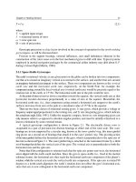
- Example 3.7.2

Response in the Form 𝐴𝑠𝑖𝑛(𝜔𝑡 + 𝜑)
3𝑠 + 10
𝑠 2 + 16
obtain 𝑓(𝑡) in the form 𝑓(𝑡) = 𝐴𝑠𝑖𝑛(𝜔𝑡 + 𝜑), where 𝐴 > 0
Solution
𝑠𝑠𝑖𝑛𝜙 + 𝜔𝑐𝑜𝑠𝜙
ℒ 𝐴𝑠𝑖𝑛 𝜔𝑡 + 𝜙 = 𝐴
𝑠2 + 𝜔2
Comparing this with 𝐹(𝑠) to get 𝑠𝑖𝑛𝜙 = 3/𝐴, 𝑐𝑜𝑠𝜙 = 5/(2𝐴)
𝑠𝑖𝑛𝜙
3/𝐴
3
𝜙 = 𝑡𝑎𝑛−1
= 𝑡𝑎𝑛−1
= 𝑡𝑎𝑛−1
− 0.876𝑟𝑎𝑑

𝑐𝑜𝑠𝜙
10/4𝐴
10/4
2
2
3
10
𝑠𝑖𝑛2 𝜙 + 𝑐𝑜𝑠 2 =
+
= 1 ⟹ 𝐴 = 61/2
𝐴
4𝐴
The solution is
𝑓 𝑡 = 0.5 61𝑠𝑖𝑛(4𝑡 + 0.876)
Given that

𝐹 𝑠 =

HCM City Univ. of Technology, Faculty of Mechanical Engineering

System Dynamics

3.111

Nguyen Tan Tien

Fluid and Thermal Systems

§7.Additional Examples
This can be expressed as a single fraction as follows

𝐶1 (𝑠 + 2)2 +25 + 𝐶2 𝑠(𝑠𝑠𝑖𝑛𝜙 + 2𝑠𝑖𝑛𝜙 + 5𝑐𝑜𝑠𝜙)
𝑋 𝑠 =
𝑠 (𝑠 + 2)2 +25
𝐶1 + 𝐶2𝑠𝑖𝑛𝜙 𝑠2 + 4𝐶1 + 2𝐶2𝑠𝑖𝑛𝜙 + 5𝐶2𝑐𝑜𝑠𝜙 𝑠 + 29𝐶1
=
(2)
𝑠 (𝑠 + 2)2+25
Comparing the numerators of eq.s (1) and (2)
𝐶1 + 𝐶2 𝑠𝑖𝑛𝜙 = 2
𝐶 = 0.0575
4𝐶1 + 2𝐶2𝑠𝑖𝑛𝜙 + 5𝐶2 𝑐𝑜𝑠𝜙 = 15 ⟹ 1
𝐶2 = 2.918
29𝐶1 = 5/3
Thus the solution is
𝑥 𝑡 = 0.0575 + 2.918𝑒 −2𝑡 𝑠𝑖𝑛(5𝑡 + 0.729)

HCM City Univ. of Technology, Faculty of Mechanical Engineering

System Dynamics

3.113

Nguyen Tan Tien

Fluid and Thermal Systems

§7.Additional Examples
From the shifting property
𝑥 𝑡 = 𝑦 𝑡 𝑢𝑠 𝑡 − 𝑦 𝑡 − 2 𝑢𝑠 (𝑡 − 2)
(1)

To find 𝑦(𝑡), note that the denominator roots of 𝑌(𝑠) are 𝑠 = 0
and 𝑠 = −4. Thus we can express 𝑌(𝑠) as follows
𝐶1
𝐶2
1 1
1
1 1
𝑌 𝑠 = +
=
−
⟹ 𝑦 𝑡 = − 𝑒 −4𝑡
𝑠 𝑠+4 4 𝑠 𝑠+4
4 4
and from eq.(1)
1 1 −4𝑡
1 1
𝑥 𝑡 =
− 𝑒
− − 𝑒 −4 𝑡−2 𝑢𝑠 (𝑡 − 2)
4 4
4 4
1 1
So for 0 ≤ 𝑡 ≤ 2
𝑥 𝑡 = − 𝑒 −4𝑡
4 4
1 1
1 1
for
𝑡>2
𝑥 𝑡 = − 𝑒 −4𝑡 − + 𝑒 −4 𝑡−2

4 4
4 4
= 0.25 𝑒 −4(𝑡−2) − 𝑒 −4𝑡
HCM City Univ. of Technology, Faculty of Mechanical Engineering

System Dynamics

3.110

The roots are 𝑠 = 0, 𝑠 = −2 ± 5𝑗, the form of the solution is
𝑥 𝑡 = 𝐶1 + 𝐶2 𝑒 −2𝑡 𝑠𝑖𝑛(5𝑡 + 𝜙)
1
𝑠𝑠𝑖𝑛𝜙 + 2𝑠𝑖𝑛𝜙 + 5𝑐𝑜𝑠𝜙
⟹ 𝑋 𝑠 = 𝐶1 + 𝐶2
𝑠
(𝑠 + 2)2 +25
HCM City Univ. of Technology, Faculty of Mechanical Engineering

System Dynamics

3.112

Nguyen Tan Tien

Fluid and Thermal Systems

§7.Additional Examples
- Example 3.7.4
Pulse Response of a First-Order Model
Suppose a rectangular pulse 𝑃(𝑡) of unit height and duration 2

is applied to the first-order model 𝑥 + 4𝑥 = 𝑃(𝑡), 𝑥 0 = 0. Use
the Laplace transform to determine the response
Solution
Taking the transform of both sides of the equation and noting
that the initial condition is zero, we obtain
1 − 𝑒 −2𝑠
𝑠𝑋 𝑠 + 4𝑋 𝑠 = 𝑃 𝑠 =
𝑠
Solve for 𝑋(𝑠)
𝑃(𝑠) 1 − 𝑒 −2𝑠
𝑋 𝑠 =
=
𝑠 + 4 𝑠(𝑠 + 4)
1
Let 𝑌 𝑠 ≡
⟹ 𝑋 𝑠 = 1 − 𝑒 −2𝑠 𝑌 𝑠
𝑠(𝑠 + 4)
HCM City Univ. of Technology, Faculty of Mechanical Engineering

System Dynamics

3.114

Nguyen Tan Tien

Fluid and Thermal Systems

§7.Additional Examples

So for 0 ≤ 𝑡 ≤ 2

for

Nguyen Tan Tien

Fluid and Thermal Systems

§7.Additional Examples
- Example 3.7.3
Sine Form of the Response
Obtain the solution to the following problem in the form of a
sine function with a phase angle
3𝑥 + 12𝑥 + 87𝑥 = 5,
𝑥 0 = 2, 𝑥 0 = 7
Solution
Applying the Laplace transform we obtain
3 𝑠2𝑋 𝑠 − 𝑠𝑥 0 − 𝑥(0) + 12 𝑠𝑋 𝑠 − 𝑥(0) + 87𝑋 𝑠 = 5/𝑠
6𝑠 2 + 45𝑠 + 5
2𝑠 2 + 15𝑠 + 5/3
⟹𝑋 𝑠 =
=
(1)
3𝑠(𝑠 2 + 4𝑠 + 29)
𝑠 (𝑠 + 2)2 +25

𝑡>2

1 1 −4𝑡
− 𝑒
4 4
1 1 −4𝑡 1 1 −4

𝑥 𝑡 = − 𝑒
− + 𝑒
4 4
4 4
−4(𝑡−2)
= 0.25 𝑒
− 𝑒 −4𝑡

𝑥 𝑡 =

HCM City Univ. of Technology, Faculty of Mechanical Engineering

𝑡−2

Nguyen Tan Tien

19


8/25/2013

System Dynamics

3.115

Fluid and Thermal Systems

System Dynamics

3.116

Fluid and Thermal Systems

§7.Additional Examples
- Example 3.7.5
Series Solution Method
Obtain an approximate, closed-form solution of the following
problem for 0 ≤ 𝑡 ≤ 0.5:
𝑥 + 𝑥 = 𝑡𝑎𝑛𝑡, 𝑥 0 = 0
Solution
Use separation of variables to solve this problem we obtain
𝑑𝑡
𝑥 + 𝑥 = 𝑡𝑎𝑛𝑡 ⟹
= 𝑑𝑡
𝑡𝑎𝑛𝑡 − 𝑥
so the variables do not separate. In general, when the input is a
function of time, the equation 𝑥 + 𝑔(𝑥) = 𝑓(𝑡) does not separate
The Laplace transform method cannot be used when the
Laplace transform or inverse transform either does not exist or
cannot be found easily. In this example, the equation cannot
be solved by the Laplace transform method, because the
transform of 𝑡𝑎𝑛𝑡 does not exist

§7.Additional Examples
An approximate solution of the equation 𝑥 + 𝑥 = 𝑡𝑎𝑛𝑡 can be
obtained by replacing 𝑡𝑎𝑛𝑡 with a series approximation
𝑡 3 2𝑡 5 17𝑡 7
𝜋
𝑡𝑎𝑛𝑡 = 𝑡 + +
+

+⋯ ,
𝑡 <
3
15
315
2
Using the two-term series to solve the following problem
𝑡3
𝑥+𝑥 =𝑡+ ,
𝑥 0 =0
3
Using the Laplace transform we obtain
1 1 3!
𝑠𝑋 𝑠 + 𝑋 𝑠 = 2 + 4
𝑠
3𝑠
𝑠2 + 2
2
2
3 3
3
⟹ 𝑋(𝑠) = 4
= 4− 3+ 2− +
𝑠 (𝑠 + 1) 𝑠
𝑠
𝑠
𝑠 𝑠+1
1
⟹ 𝑥 𝑡 = 𝑡 3 − 𝑡 2 + 3𝑡 − 3 + 3𝑒 −𝑡
3

HCM City Univ. of Technology, Faculty of Mechanical Engineering

HCM City Univ. of Technology, Faculty of Mechanical Engineering

System Dynamics

Nguyen Tan Tien

3.117

Fluid and Thermal Systems

§8.Computing Expansion Coefficients with Matlab
- Example 8.1
Real, Distinct Poles
6𝑠 3 + 57𝑠 2 + 120𝑠 + 80
𝑋 𝑠 =
𝑠 2 + 9𝑠 + 14
Solution
Matlab [r,p,K] = residue([6,57,120,80],[1,9,14])
Result
r = [5, 4], p = [−7, −2], K = [6, 3]
𝑋 𝑠 = 6𝑠 + 3 +

9𝑠 + 38
1
1
= 6 𝑠+ 3 +5
+4

𝑠 2 + 9𝑠 + 14 𝑘
𝑠 − (−7) 𝑟 𝑠 − (−2)
𝑘
𝑟
1

2

1

𝑝1

HCM City Univ. of Technology, Faculty of Mechanical Engineering

System Dynamics

1

Fluid and Thermal Systems

§8.Computing Expansion Coefficients with Matlab
- Example 8.3
Complex Poles
4𝑠 + 1
𝑋 𝑠 = 3
𝑠 + 6𝑠 2 + 34𝑠
Solution
Matlab [r,p,K] = residue([4,1],[1,6,34,0])
Result
r = [−0.0147 − 0.3912𝑖, −0.0147 + 0.3912𝑖, 0.0294]

p = [−3 + 5𝑖, −3 − 5𝑖, 0]
K=[]
𝑟1

𝑟2

𝑟3

−0.0147 − 0.3912𝑗 −0.0147 + 0.3912𝑗 0.0294
𝑋 𝑠 =
+
+
𝑠 − (−3 + 5𝑗)
𝑠 − (−3 − 5𝑗)
𝑠− 0
𝑝1

HCM City Univ. of Technology, Faculty of Mechanical Engineering

𝑝2

𝑝3

Nguyen Tan Tien

3.118

Fluid and Thermal Systems

§8.Computing Expansion Coefficients with Matlab

- Example 8.2
Repeated Poles
12𝑠 + 8
𝑋 𝑠 = 3
𝑠 + 16𝑠 2 + 77𝑠 + 98
Solution
Matlab [r,p,K] = residue([12,8],[1,16,77,98])
Result
r =[0.64, 15.2, −0.64], p = [−7, −7, −2], K = [ ]
𝑋 𝑠 = 0 + 0.64
𝑘

𝑝2

Nguyen Tan Tien

3.119

System Dynamics

Nguyen Tan Tien

𝑟1

1
1
1
+ 1.52
+ (−0.64)
𝑠 − (−7)

[𝑠 − (−7)]2
𝑠 − (−2)
𝑟
𝑟
𝑝1

2

HCM City Univ. of Technology, Faculty of Mechanical Engineering

System Dynamics

3.120

𝑝2

3

𝑝3

Nguyen Tan Tien

Fluid and Thermal Systems

§9.Transfer Function Analysis in Matlab
1.The tf and tfdata function
tf
creation of TF or conversion to TF
tfdata quick access to TF data
Example

𝑋(𝑠)
1
=
𝐹(𝑠) 5𝑠 2 + 9𝑠 + 4
Solution
Matlab sys1 = tf(1, [5, 9, 4])
Example
𝑑3𝑥
𝑑2𝑥
𝑑𝑥
𝑑2𝑓
𝑑𝑓
5 3 +4 2 +7
+ 3𝑥 = 6 2 + 9
+ 2𝑓
𝑑𝑡
𝑑𝑡
𝑑𝑡
𝑑𝑡
𝑑𝑡
Solution
Matlab sys2 = tf([6, 9, 2],[5, 4, 7, 3])
HCM City Univ. of Technology, Faculty of Mechanical Engineering

Nguyen Tan Tien

20


8/25/2013

System Dynamics

3.121

Fluid and Thermal Systems

System Dynamics

3.122

Fluid and Thermal Systems

§9.Transfer Function Analysis in Matlab
2.ODE Solvers
- The Control System Toolbox provides several solvers for
linear models. These solvers are categorized by the type of
input function they can accept: some of these are a step
input, an impulse input, and a general input function
- Example 3.9.1
Step Response of a Second-Order Model
𝑋(𝑠)
𝑐𝑠 + 5
Consider the model
, plot
=
𝐹(𝑠) 10𝑠 2 + 𝑐𝑠 + 5
a. The unit-step response for 𝑐 = 3 using the time span
selected by Matlab
b. The unit-step response for 𝑐 = 3 over the range 0 ≤ 𝑡 ≤ 15

c. The unit-step responses for 𝑐 = 3 and 𝑐 = 8 over the
range 0 ≤ 𝑡 ≤ 15. Put the plots on the same graph
d. The step response for 𝑐 = 3, where the magnitude of the
step input is 20. Use the time span selected by Matlab

§9.Transfer Function Analysis in Matlab
a. The unit-step response for 𝑐 = 3 using the time span
selected by Matlab
Matlab sys1 = tf([3,5],[10,3,5]);
step(sys1)

HCM City Univ. of Technology, Faculty of Mechanical Engineering

HCM City Univ. of Technology, Faculty of Mechanical Engineering

System Dynamics

3.123

Nguyen Tan Tien

Fluid and Thermal Systems

System Dynamics

3.124

Nguyen Tan Tien

Fluid and Thermal Systems

§9.Transfer Function Analysis in Matlab
b. The unit-step response for 𝑐 = 3 over the range 0 ≤ 𝑡 ≤ 15
Matlab sys1 = tf([3,5],[10,3,5]);
t = (0:0.01:15);
step(sys1)

§9.Transfer Function Analysis in Matlab
c. The unit-step responses for 𝑐 = 3 and 𝑐 = 8 over the
range 0 ≤ 𝑡 ≤ 15. Put the plots on the same graph
Matlab sys1 = tf([3,5],[10,3,5]);
sys2 = tf([8,5],[10,8,5]);
t = (0:0.01:15);
step(sys1,' ',sys2,'--',t)

HCM City Univ. of Technology, Faculty of Mechanical Engineering

HCM City Univ. of Technology, Faculty of Mechanical Engineering

System Dynamics

3.125

Nguyen Tan Tien

Fluid and Thermal Systems

System Dynamics

3.126

Nguyen Tan Tien

Fluid and Thermal Systems

§9.Transfer Function Analysis in Matlab
d. The step response for 𝑐 = 3, where the magnitude of the
step input is 20. Use the time span selected by Matlab
Matlab sys1 = tf([3,5],[10,3,5]);
[y, t] = step(sys1);
plot(t,20*y),xlabel('t'),ylabel('x(t)')

§9.Transfer Function Analysis in Matlab
- Example 3.9.2 Impulse Response of Second-Order Models
Obtained the response of the following model to a unit
impulse
𝑋(𝑠)
1
=
𝐹(𝑠) 2𝑠 2 + 14𝑠 + 20
Our analysis showed that if 𝑥(0) = 𝑥(0) = 0, then 𝑥 0+ = 0
and 𝑥 0+ = 1/2. Use the impulse function to verify these
results
Solution
Matlab sys1 = tf(1,[2, 14, 20]);
impulse(sys1)

HCM City Univ. of Technology, Faculty of Mechanical Engineering

HCM City Univ. of Technology, Faculty of Mechanical Engineering

Nguyen Tan Tien

Nguyen Tan Tien

21


8/25/2013

System Dynamics

3.127

Fluid and Thermal Systems

System Dynamics

3.128

§9.Transfer Function Analysis in Matlab
From the plot we see that𝑥 0+ = 0 and that 𝑥 0+ is positive
as predicted. We are unable to determine the exact value of
𝑥 0+ from this plot, so we multiply the transfer function by 𝑠
to obtain the transfer function for 𝑣 = 𝑥

§9.Transfer Function Analysis in Matlab
𝑉(𝑠)
𝑠
=

𝐹(𝑠) 2𝑠 2 + 14𝑠 + 20
Matlab sys2 = tf([1,0],[2, 14, 20]);
impulse(sys1)

HCM City Univ. of Technology, Faculty of Mechanical Engineering

HCM City Univ. of Technology, Faculty of Mechanical Engineering

Fluid and Thermal Systems

𝑥 0+ = 1/2 as predicted

System Dynamics

3.129

Nguyen Tan Tien

Fluid and Thermal Systems

System Dynamics

3.130

§9.Transfer Function Analysis in Matlab
- Example 3.9.3
Ramp Response with the lsim Function
Plot the forced response of
𝑥 + 3𝑥 + 𝑥5 = 10𝑓(𝑡)
to a ramp input, 𝑢(𝑡) = 1.5𝑡, over the time interval 0 ≤ 𝑡 ≤ 2

Solution
Matlab t = linspace(0,2,300);
f = 1.5*t;
sys = tf(10, [1, 3, 5]);
[y, t] = lsim(sys,f,t);
plot(t,y,t,f),xlabel('t'),ylabel('x(t) and f(t)')

§9.Transfer Function Analysis in Matlab
The resulting plot

HCM City Univ. of Technology, Faculty of Mechanical Engineering

HCM City Univ. of Technology, Faculty of Mechanical Engineering

Nguyen Tan Tien

Nguyen Tan Tien

Fluid and Thermal Systems

Nguyen Tan Tien

22