Ch 07 fluid and thermal systems

8/25/2013

System Dynamics

7.01

Fluid and Thermal Systems

7. Fluid and Thermal Systems

HCM City Univ. of Technology, Faculty of Mechanical Engineering

System Dynamics

7.03

Nguyen Tan Tien

Fluid and Thermal Systems

System Dynamics

7.02

Part 1. Fluid Systems

HCM City Univ. of Technology, Faculty of Mechanical Engineering

System Dynamics

7.04

§1.Conservation of Mass
For incompressible fluids
conservation of mass ⟺ conservation of volume
The mass flow rate
𝑞𝑚 = 𝜌𝑞𝑣
𝜌: fluid density, 𝑘𝑔/𝑚3
𝑞𝑚 : the mass flow rates, 𝑘𝑔/𝑠
𝑞𝑣 : the volume flow rate, 𝑚3 /𝑠
1.Density and Pressure
- Density (mass density): mass per unit volume, 𝑘𝑔/𝑚3
- Pressure: force per unit area that is exerted by the fluid, 𝑁/𝑚2
- Hydrostatic pressure: the pressure that exists in a fluid at rest

§1.Conservation of Mass
- Example 7.1.1

HCM City Univ. of Technology, Faculty of Mechanical Engineering

HCM City Univ. of Technology, Faculty of Mechanical Engineering

System Dynamics

7.05

Nguyen Tan Tien

Fluid and Thermal Systems

§1.Conservation of Mass

Solution
The forces are related to the
pressures and the piston areas
𝑓1 = 𝑝1 𝐴1 ,
𝑓2 = 𝑝2 𝐴2
Assuming the system is in static
equilibrium after the brake pedal
has been pushed
𝑝1 = 𝑝2 + 𝜌𝑔ℎ ≈ 𝑝2
𝑓1
𝑓2
𝐴2
⟹ 𝑝1 =
= 𝑝2 =
⟹ 𝑓2 = 𝑓1
𝐴1
𝐴2
𝐴1
The force 𝑓3
𝐿1 𝐴2 𝐿1
𝑓3 = 𝑓2 =
𝑓
𝐿2 𝐴1 𝐿2 1
HCM City Univ. of Technology, Faculty of Mechanical Engineering

Nguyen Tan Tien

Fluid and Thermal Systems

Nguyen Tan Tien

Fluid and Thermal Systems

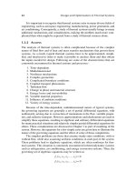
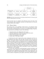
A Hydraulic Brake System
The figure is a representation of a
hydraulic brake system. The piston
in the master cylinder moves in
response to the foot pedal. The
resulting motion of the piston in the
slave cylinder causes the brake
pad to be pressed against the
brake drum with a force 𝑓3 . The
force 𝑓1 depends on the force 𝑓4
applied by the driver’s foot. The
precise relation between 𝑓1 and 𝑓4
depends on the geometry of the
pedal arm
Obtain the expression for the force 𝑓3 with the force 𝑓1 as the input

System Dynamics

7.06

Nguyen Tan Tien

Fluid and Thermal Systems

§1.Conservation of Mass
- Conservation of mass
𝑚 = 𝑞𝑚𝑖 − 𝑞𝑚𝑜

𝑞𝑚𝑖 : the mass inflow rate, 𝑘𝑔/𝑠
𝑞𝑚𝑜 : the mass outflow rate , 𝑘𝑔/𝑠
𝑞𝑚𝑖 = 𝜌𝑞𝑣𝑖
𝑞𝑚𝑜 = 𝜌𝑞𝑣𝑜
𝑞𝑣𝑖 : total volume inflow rate, 𝑚3 /𝑠
𝑞𝑣𝑜 : total volume inflow rate, 𝑚3 /𝑠
- The fluid mass 𝑚 is related to the container volume 𝑉
𝑚 = 𝜌𝑉 ⟹ 𝑚 = 𝜌𝑉
then
𝜌𝑉 = 𝜌𝑞𝑣𝑖 − 𝜌𝑞𝑣𝑜
⟹ 𝑉 = 𝑞𝑣𝑖 − 𝑞𝑣𝑜
This is a statement of conservation of volume for the fluid
HCM City Univ. of Technology, Faculty of Mechanical Engineering

Nguyen Tan Tien

1


8/25/2013

System Dynamics

§1.Conservation of Mass
- Example 7.1.2

7.07

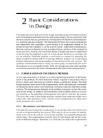
A Water Supply Tank
Water is pumped at the mass flow rate

𝑞𝑚𝑜 (𝑡) from the tank. Replacement
water is pumped from a well at the
mass flow rate 𝑞𝑚𝑖 (𝑡). Determine the
water height ℎ(𝑡), assuming that the
tank is cylindrical with a cross section 𝐴
Solution
From conservation of mass
𝑑
𝜌𝐴ℎ = 𝑞𝑚𝑖 𝑡 − 𝑞𝑚𝑜 𝑡
𝑑𝑡
𝑑ℎ
⟹ 𝜌𝐴
= 𝑞𝑚𝑖 𝑡 − 𝑞𝑚𝑜 𝑡
𝑑𝑡
1 𝑡
⟹ℎ 𝑡 =ℎ 0 +
[𝑞 𝑢 − 𝑞𝑚𝑜(𝑢)]𝑑𝑢
𝜌𝐴 0 𝑚𝑖

HCM City Univ. of Technology, Faculty of Mechanical Engineering

System Dynamics

Fluid and Thermal Systems

7.09

Nguyen Tan Tien

Fluid and Thermal Systems

§1.Conservation of Mass
Solution
a.Model of the motion for figure (a)
Assuming that 𝑝1 > 𝑝2 , the net force
acting on the piston and mass 𝑚 is (𝑝1 −
𝑝2 )𝐴, and thus from Newton’s law
𝑚𝑥 = (𝑝1 − 𝑝2 )𝐴
Integrate this equation once to obtain the velocity
𝐴 𝑡
𝑥 𝑡 =𝑥 0 +
[𝑝 𝑢 − 𝑝2 (𝑢)]𝑑𝑢
𝑚 0 1
The rate at which fluid volume is swept out by the piston is
𝐴𝑥, and thus if 𝑥 > 0, the pump providing pressure 𝑝1 must
supply fluid at the mass rate 𝜌𝐴𝑥, and the pump providing
pressure 𝑝2 must absorb fluid at the same mass rate
HCM City Univ. of Technology, Faculty of Mechanical Engineering

System Dynamics

7.11

Nguyen Tan Tien

Fluid and Thermal Systems

System Dynamics

7.08

Fluid and Thermal Systems

§1.Conservation of Mass
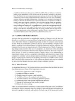
- Example 7.1.3

A Hydraulic Cylinder
Fig.(a): a cylinder and piston connected
to a load mass 𝑚
Fig.(b): the piston rod connected to a
rack-and-pinion gear
The pressures 𝑝1 and 𝑝2 are applied to
each side of the piston by two pumps.
Neglect the piston rod diameter and
assume that the piston and rod mass
have been lumped into 𝑚
a.Develop a model of the motion of the displacement 𝑥 of the
mass in fig.(a). Also, obtain the expression for the mass flow
rate that must be delivered or absorbed by the two pumps
b.Develop a model of the displacement 𝑥 in fig.(b). The inertia
of the pinion and the load connected to the pinion is 𝐼

HCM City Univ. of Technology, Faculty of Mechanical Engineering

System Dynamics

7.10

Nguyen Tan Tien

Fluid and Thermal Systems

§1.Conservation of Mass
Solution
b.Model of the motion for figure (b)
Firstly, obtain an expression for the equivalent mass of the
rack, pinion, and load. The kinetic energy of the system is
1
1
1
𝐼
𝐾𝐸 = 𝑚𝑥 2 + 𝐼𝜃 2 = 𝑚 + 2 𝑥 2
2
2
2
𝑅
because 𝑅𝜃 = 𝑥
Thus the equivalent mass is
𝐼
𝑚𝑒 = 𝑚 + 2
𝑅
Then, the required model can now be obtained by replacing
𝑚 with 𝑚𝑒 in the model developed in part (a)

HCM City Univ. of Technology, Faculty of Mechanical Engineering

System Dynamics

7.12

Nguyen Tan Tien

Fluid and Thermal Systems

§1.Conservation of Mass
- Example 7.1.4
A Mixing Process
A mixing tank is shown in the figure. Pure water
flows into the tank of volume 𝑉 = 600𝑚3 at the
constant volume rate of 5𝑚3 /𝑠. A solution with a
salt concentration of 𝑠𝑖 𝑘𝑔/𝑚3 flows into the tank
at a constant volume rate of 2𝑚3 /𝑠. Assume that
the solution in the tank is well mixed so that the
salt concentration in the tank is uniform. Assume
also that the salt dissolves completely so that the
volume of the mixture remains the same.
The salt concentration 𝑠𝑜 𝑘𝑔/𝑚3 in the outflow is the same as
the concentration in the tank. The input is the concentration
𝑠𝑖 (𝑡) , whose value may change during the process, thus
changing the value of 𝑠𝑜 . Obtain a dynamic model of the
concentration 𝑠𝑜

§1.Conservation of Mass
Solution
Two mass species are conserved here: water
mass and salt mass. The tank is always full, so
the mass of water 𝑚𝑤 in the tank is constant, and
thus conservation of water mass gives
𝑑𝑚𝑤
= 5𝜌𝑤 + 2𝜌𝑤 − 𝜌𝑤 𝑞𝑣𝑜 = 0 ⟹ 𝑞𝑣𝑜 = 7𝑚3 /𝑠

𝑑𝑡
𝜌𝑤 : the mass density of fresh water
𝑞𝑣𝑜 : the volume outflow rate of the mixed solution
The salt mass in the tank is 𝑠𝑜 𝑉, and conservation of salt mass
gives
𝑑
𝑑𝑠𝑜 2𝑠𝑖 − 7𝑠𝑜
𝑠 𝑉 = 0 5 + 2𝑠𝑖 − 𝑠𝑜 𝑞𝑣𝑜 = 2𝑠𝑖 − 7𝑠𝑜 ⟹
=
𝑑𝑡 𝑜
𝑑𝑡
600

HCM City Univ. of Technology, Faculty of Mechanical Engineering

HCM City Univ. of Technology, Faculty of Mechanical Engineering

Nguyen Tan Tien

Nguyen Tan Tien

2


8/25/2013

System Dynamics

7.13

Fluid and Thermal Systems

§2.Fluid Capacitance
- Sometimes it is very useful to think of fluid systems in terms of
electrical circuits
Fluid mass,
Mass flow rate,

𝑚
𝑞𝑚

Charge,
Current,

Pressure,
𝑝
Fluid linear resistance,𝑅 = 𝑝/𝑞𝑚
Fluid capacitance, 𝐶 = 𝑚/𝑝
Fluid inertance,

𝑄
𝑖

Voltage,
𝑣
Electrical resistance, 𝑅 = 𝑣/𝑖
Electrical capacitance, 𝐶 = 𝑄/𝑣

𝐼 = 𝑝/(𝑑𝑞𝑚/𝑑𝑡) Electrical inductance, 𝐿 = 𝑣/(𝑑𝑖/𝑑𝑡)

- Fluid resistance is the relation between pressure and mass
flow rate. Fluid resistance relates to energy dissipation
- Fluid capacitance is the relation between pressure and stored
mass. Fluid capacitance relates to potential energy
- Fluid inertance relates to fluid acceleration and kinetic energy
HCM City Univ. of Technology, Faculty of Mechanical Engineering

System Dynamics

Nguyen Tan Tien

7.15

Fluid and Thermal Systems

§2.Fluid Capacitance
1.Fluid Symbols and Source
- Resistance
Both linear and nonlinear fixed resistances, for
example, pipe flow, orifice flow, or a restriction
- Valve
• manually adjusted valve: faucet
• actuated valve: driven by an electric motor or a
pneumatic device

System Dynamics

7.14

Fluid and Thermal Systems

§2.Fluid Capacitance
- Fluid systems obey two laws that are analogous to Kirchhoff’s
current and voltage laws
• The continuity law (conservation of fluid mass): the total mass
flow into a junction must equal the total flow out of the junction
• The compatibility law (conservation of energy): the sum of
signed pressure differences around a closed loop must be
zero
- Note: the flow is through flexible tubes that can expand and
contract under pressure, then the outflow rate is not the sum of
the inflow rates. This is an example where fluid mass can
accumulate within the system and is analogous to having a
capacitor in an electrical circuit

HCM City Univ. of Technology, Faculty of Mechanical Engineering

System Dynamics

7.16

Nguyen Tan Tien

Fluid and Thermal Systems

§2.Fluid Capacitance
- Ideal pressure source
Supplying the specified pressure at any flow rate

- Ideal flow source

Supplying the specified flow

- Pump
Ideal sources are approximations to real devices
such as pumps
HCM City Univ. of Technology, Faculty of Mechanical Engineering

System Dynamics

Nguyen Tan Tien

7.17

Fluid and Thermal Systems

§2.Fluid Capacitance
2.Capacitance Relations
- The figure illustrates the relation
between stored fluid mass and the
resulting pressure caused by the stored
mass
- Fluid capacitance 𝐶 : the ratio of the
change in stored mass to the change in
pressure
𝑑𝑚
𝐶≡
𝑑𝑝 𝑝=𝑝
𝑟

𝑚: the stored fluid mass, 𝑘𝑔

𝑝: the resulting pressure, 𝑁/𝑚2

HCM City Univ. of Technology, Faculty of Mechanical Engineering

Nguyen Tan Tien

HCM City Univ. of Technology, Faculty of Mechanical Engineering

System Dynamics

§2.Fluid Capacitance
- Example 7.2.1

7.18

Nguyen Tan Tien

Fluid and Thermal Systems

Capacitance of a Storage Tank
Consider the tank shown in the
figure. Assume that the cross
sectional area 𝐴 is constant.
Derive the expression for the
tank’s capacitance

Solution
The liquid mass in the tank:
The total pressure at the bottom of the tank:
Pressure due only to the stored fluid mass:

The pressure function of the mass 𝑚:
The capacitance of the tank is given by
𝑑𝑚 𝐴
𝐶≡
=
𝑑𝑝 𝑔
HCM City Univ. of Technology, Faculty of Mechanical Engineering

𝑚 = 𝜌𝐴ℎ
𝜌𝑔ℎ + 𝑝𝑎
𝑝 = 𝜌𝑔ℎ
𝑝 = 𝑚𝑔/𝐴

Nguyen Tan Tien

3


8/25/2013

System Dynamics

7.19

Fluid and Thermal Systems

§2.Fluid Capacitance
- When the container does not
have vertical sides, the crosssectional area 𝐴 is a function of
the liquid height ℎ , and the

relations between 𝑚 and ℎ and
between 𝑝 and 𝑚 are nonlinear
- The fluid mass stored in the container
ℎ
𝑑𝑚
𝑚 = 𝜌𝑉 = 𝜌 𝐴 𝑥 𝑑𝑥 ⟹
= 𝜌𝐴
𝑑ℎ
0
- For such a container, conservation of mass gives
𝑑𝑚
𝑑𝑚 𝑑𝑚 𝑑𝑝
𝑑𝑝
= 𝑞𝑚𝑖 − 𝑞𝑚𝑜 ⟹
=
=𝐶
= 𝑞𝑚𝑖 − 𝑞𝑚𝑜
𝑑𝑡
𝑑𝑡
𝑑𝑝 𝑑𝑡
𝑑𝑡
- Also
𝑑𝑚 𝑑𝑚 𝑑ℎ
𝑑ℎ
𝑑ℎ
=
= 𝜌𝐴
⟹ 𝜌𝐴
= 𝑞𝑚𝑖 − 𝑞𝑚𝑜
𝑑𝑡

𝑑ℎ 𝑑𝑡
𝑑𝑡
𝑑𝑡
HCM City Univ. of Technology, Faculty of Mechanical Engineering

System Dynamics

7.21

Nguyen Tan Tien

Fluid and Thermal Systems

§2.Fluid Capacitance
b. Dynamic Model

which is a nonlinear equation because of the
product 𝑝𝑝
Obtain the model for the height by
substituting ℎ = 𝑝/𝜌𝑔
𝑑ℎ
2𝜌𝐿𝑡𝑎𝑛𝜃 ℎ
= 𝑞𝑚𝑖
𝑑𝑡

HCM City Univ. of Technology, Faculty of Mechanical Engineering

7.23

Nguyen Tan Tien

Fluid and Thermal Systems

§3.Fluid Resistance
- The relation 𝑝 = 𝑓(𝑞𝑚 )
• is linear in a limited number of cases, such as pipe flow
under certain conditions
𝑞𝑚 = 𝑝/𝑅
• is a square-root relation in some other applications
𝑞𝑚 =

7.20

Fluid and Thermal Systems

§2.Fluid Capacitance
- Example 7.2.2
Capacitance of a V-Shaped Trough
a. Derive the capacitance of the V-shaped
b. Derive the dynamic models for the bottom
pressure 𝑝 and the height ℎ. The mass inflow
rate is 𝑞𝑚𝑖 (𝑡)
Solution
a. The fluid mass
1
𝑚 = 𝜌𝑉 = 𝜌 ℎ𝐷 𝐿 = 𝜌𝐿𝑡𝑎𝑛𝜃 ℎ2
2
2
𝑝
𝐿𝑡𝑎𝑛𝜃 2

= 𝜌𝐿𝑡𝑎𝑛𝜃
=
𝑝
𝜌𝑔
𝜌𝑔2
From the definition of capacitance
𝑑𝑚
2𝐿𝑡𝑎𝑛𝜃
𝐶=
=
𝑝
𝑑𝑝
𝜌𝑔2
HCM City Univ. of Technology, Faculty of Mechanical Engineering

System Dynamics

7.22

Nguyen Tan Tien

Fluid and Thermal Systems

§3.Fluid Resistance

𝑑𝑝 𝑑𝑚
𝐶
=
= 𝑞𝑚𝑖 − 𝑞𝑚𝑜
𝑑𝑡

𝑑𝑡
with 𝑞𝑚𝑜 = 0, 𝐶 = 𝑝 = 𝑞𝑚𝑖
2𝐿𝑡𝑎𝑛𝜃 𝑑𝑝
𝑝
= 𝑞𝑚𝑖
𝜌𝑔2
𝑑𝑡

System Dynamics

System Dynamics

𝑝
𝑅1

𝑚𝑟

the reference values of 𝑞𝑚𝑟 and 𝑝𝑟 depend on the particular
application
HCM City Univ. of Technology, Faculty of Mechanical Engineering

System Dynamics

𝑅𝑟 : the linearized resistance at the reference condition (𝑞𝑚𝑟 , 𝑝𝑟 )
Nguyen Tan Tien

7.24

Nguyen Tan Tien

Fluid and Thermal Systems

§3.Fluid Resistance
- Deviation variable at the reference values of 𝑞𝑚𝑟 and 𝑝𝑟
𝛿𝑝 ≡ 𝑝 − 𝑝𝑟
𝛿𝑞𝑚 ≡ 𝑞𝑚 − 𝑞𝑚𝑟
⟹ 𝛿𝑝 = 𝑅𝑟 𝛿𝑞𝑚 = 2𝑅1
⟹ 𝛿𝑞𝑚 =

• can be linearized the expression near a reference operating
point (𝑞𝑚𝑟 , 𝑝𝑟 )
𝑑𝑝
𝑝 = 𝑝𝑟 +
𝑞 − 𝑞𝑚𝑟 = 𝑝𝑟 + 𝑅𝑟 𝑞𝑚 − 𝑞𝑚𝑟
𝑑𝑞𝑚 𝑟 𝑚

HCM City Univ. of Technology, Faculty of Mechanical Engineering

- Fluid meets resistance when flowing
through a conduit such as a pipe, through a
component such as a valve, or even
through a simple opening or orifice, such as
a hole
- The relation between mass flow rate 𝑞𝑚 and
the pressure difference 𝑝 across the
resistance 𝑝 = 𝑓(𝑞𝑚 ) is shown in the figure
- Define the fluid resistance 𝑅
𝑑𝑝
𝑅≡
𝑑𝑞𝑚 𝑞=𝑞

1
2 𝑅1𝑝𝑟

𝑝𝑟
𝛿𝑞 = 2 𝑅1 𝑝𝑟 𝛿𝑞𝑚
𝑅1 𝑚

𝛿𝑝

- The resistance symbol
• series resistances
• parallel resistances
HCM City Univ. of Technology, Faculty of Mechanical Engineering

Nguyen Tan Tien

4


8/25/2013

System Dynamics

7.25

Fluid and Thermal Systems

§3.Fluid Resistance
1.Laminar Pipe Resistance

- Fluid motion is generally divided into two types
• Laminar flow:

𝑅𝑒 < 2300

• Turbulent flow:

𝑅𝑒 > 2300

for circular pipe, 𝑅𝑒 ≡

𝜇

- The laminar resistance (Hagen-Poiseuille formula)
128𝜇𝐿
𝑅=
𝜋𝜌𝐷 4
𝑅: flow resistance,
𝜇: the fluid viscosity, 𝑁𝑠/𝑚2
𝐿: the length of pipe, 𝑚
𝜌: the fluid density, 𝑘𝑔/𝑚3
𝐷: the diameter of pipe, 𝑚

System Dynamics

§3.Fluid Resistance
- Example 7.3.1

7.27

Nguyen Tan Tien

Fluid and Thermal Systems

Liquid-Level System with a Flow Source
The cylindrical tank shown in the figure
has a bottom area 𝐴. The mass inflow
rate is 𝑞𝑚𝑖 (𝑡). The outlet resistance is
linear and the outlet discharges to
atmospheric pressure 𝑝𝑎 . Develop a
model of the liquid height ℎ

Slolution
Total mass in the tank is 𝑚 = 𝜌𝐴ℎ, from conservation of mass
𝑑𝑚
𝑑ℎ
1
1
= 𝜌𝐴 = 𝑞𝑚𝑖 − 𝑞𝑚𝑜,
𝑞𝑚𝑜 =
𝜌𝑔ℎ + 𝑝𝑎 − 𝑝𝑎 = 𝜌𝑔ℎ
𝑑𝑡
𝑑𝑡
𝑅
𝑅
The desired model
𝑑ℎ
𝜌𝑔
𝜌𝐴
= 𝑞𝑚𝑖 −

ℎ
𝑑𝑡
𝑅
HCM City Univ. of Technology, Faculty of Mechanical Engineering

System Dynamics

7.29

§3.Fluid Resistance
3.Torricelli’s Principle
- An orifice can simply be a hole in the side
of a tank or it can be a passage in a valve
- The mass flow rate 𝑞𝑚 through the orifice
𝑞𝑚 = 𝐶𝑑 𝐴𝑜 2𝜌𝑝 = 𝐶𝑑 𝐴𝑜 2𝜌 𝑝 =

Nguyen Tan Tien

Fluid and Thermal Systems

Fluid and Thermal Systems

- In liquid-level systems such as
shown in the figure, energy is stored
in two ways
• potential energy in the mass of
liquid in the tank
• kinetic energy in the mass of liquid flowing in the pipe
- If the mass of liquid in a pipe is small enough or is flowing at
a small enough velocity, the kinetic energy contained in it will

be negligible compared to the potential energy stored in the
liquid in the tank

HCM City Univ. of Technology, Faculty of Mechanical Engineering

System Dynamics

𝑝/𝑅𝑜

ℎ: the height of fluid, 𝑚
Nguyen Tan Tien

7.28

Nguyen Tan Tien

Fluid and Thermal Systems

§3.Fluid Resistance
- Consider the circuit model
𝑑𝑣
1
𝐶
= 𝑖𝑠 − 𝑣
𝑑𝑡
𝑅

- The fluid flow system is analogous to the electric circuit
system
• pressure difference, 𝜌𝑔ℎ

⟺ voltage difference, 𝑣
• mass flow rate, 𝑞𝑚𝑖
⟺ current, 𝑖𝑠
• resistance resists flow
⟺ resistor resists current
• capacitance stores fluid mass, 𝐴/𝑔 ⟺ capacitor stores charge, 𝐶

HCM City Univ. of Technology, Faculty of Mechanical Engineering

System Dynamics

§3.Fluid Resistance
- Example 7.3.2

𝐶𝑑 : factor,
𝐴0 : the area of the orifice, 𝑚2
𝑝: the pressure of fluid, 𝑁/𝑚2 𝜌: the fluid density, 𝑘𝑔/𝑚3
1
𝑅𝑜 : orifice resistance 𝑅𝑜 ≡
2𝜌𝐶𝑑2 𝐴𝑜2
- The volume flow rate 𝑞𝑣 through the orifice
𝑞𝑣 = 𝐶𝑑 𝐴𝑜 2𝑔 ℎ0.5

HCM City Univ. of Technology, Faculty of Mechanical Engineering

7.26

§3.Fluid Resistance
2.System Model

𝜌 𝑣𝐷

HCM City Univ. of Technology, Faculty of Mechanical Engineering

System Dynamics

7.30

Nguyen Tan Tien

Fluid and Thermal Systems

Liquid-Level System with an Orifice
The cylindrical tank shown in the figure has
a circular bottom area 𝐴. The volume inflow
rate from the flow source is 𝑞𝑣𝑖 (𝑡), a given
function of time. The orifice in the side wall
has an area 𝐴𝑜 and discharges to
atmospheric pressure 𝑝𝑎 . Develop a model
of the liquid height ℎ, assuming that ℎ1 > 𝐿

Solution
From conservation of mass and the orifice flow relation
𝑑ℎ
𝜌𝐴
= 𝜌𝑞𝑣𝑖 − 𝐶𝑑 𝐴𝑜 2𝑝𝜌
𝑑𝑡
where 𝑝 = 𝜌𝑔ℎ. Thus the model becomes
𝑑ℎ
𝐴

= 𝑞𝑣𝑖 − 𝐶𝑑 𝐴𝑜 2𝑔ℎ
𝑑𝑡
HCM City Univ. of Technology, Faculty of Mechanical Engineering

Nguyen Tan Tien

5


8/25/2013

System Dynamics

7.31

Fluid and Thermal Systems

§3.Fluid Resistance
4.Turbulance and Component Resistance
- The practical importance of the difference between laminar
and turbulent flow lies in the fact that
• laminar flow can be described by the linear relation
𝑞𝑚 = 𝑝/𝑅
• turbulent flow is described by the nonlinear relation
𝑞𝑚 =

𝑝/𝑅1

- Components, such as valves, elbow bends, couplings,
porous plugs, and changes in flow area resist flow and

usually induce turbulent flow at typical pressures, and 𝑞𝑚 =
𝑝/𝑅1 is often used to model them
- Experimentally determined values of 𝑅 are available for
common types of components
HCM City Univ. of Technology, Faculty of Mechanical Engineering

System Dynamics

7.33

Nguyen Tan Tien

Fluid and Thermal Systems

§4.Dynamic Models of Hydraulic Systems
Because the outlet resistance is linear
1
𝜌𝑔ℎ
𝑞𝑚𝑜 =
𝜌𝑔ℎ + 𝑝𝑎 − 𝑝𝑎 =
𝑅2
𝑅2
The mass inflow rate
1
𝑞𝑚𝑖 =
𝑝 + 𝑝𝑎 − 𝜌𝑔ℎ + 𝑝𝑎
𝑅1 𝑠
1
= (𝑝𝑠 − 𝜌𝑔ℎ)
𝑅1

The desired model
𝑑ℎ
1
𝜌𝑔
𝜌𝐴
=
𝑝 − 𝜌𝑔ℎ −
ℎ
𝑑𝑡 𝑅1 𝑠
𝑅2
which can be rearranged as
𝑑ℎ 1
1
1
1
𝑅1 + 𝑅2
𝜌𝐴 = 𝑝𝑠 − 𝜌𝑔
+
ℎ = 𝑝𝑠 − 𝜌𝑔
ℎ
𝑑𝑡 𝑅1
𝑅1 𝑅2
𝑅1
𝑅1𝑅2

The time constant

7.32

Fluid and Thermal Systems

§4.Dynamic Models of Hydraulic Systems
- Example 7.4.1
Liquid-Level System with a Pressure Source
Consider the system shown in the
figure. The linear resistance 𝑅
represents the pipe resistance
lumped at the outlet of the pressure
source. The bottom of the water tank
is a height 𝐿 above the pressure source. Develop a model of
the water height ℎ with the supply pressure 𝑝𝑠 and the flow
rate 𝑞𝑚𝑜 (𝑡) as the inputs
Solution
The total mass in the tank
𝑚 = 𝜌𝐴ℎ
Since 𝜌 and 𝐴 are constants, from conservation of mass
𝑑𝑚
𝑑ℎ
= 𝜌𝐴
= 𝑞𝑚𝑖 − 𝑞𝑚𝑜
𝑑𝑡
𝑑𝑡
HCM City Univ. of Technology, Faculty of Mechanical Engineering

System Dynamics

7.34

Nguyen Tan Tien

Fluid and Thermal Systems

§4.Dynamic Models of Hydraulic Systems
- Example 7.4.2
Water Tank Model
Consider the system shown in the
figure, the input was the specified flow
rate 𝑞𝑚𝑖 . The linear resistance 𝑅
represents at the outlet of the pressure
source. The bottom of the water tank is
a height 𝐿 above the pressure source.
Develop a model of the water height ℎ with the supply
pressure 𝑝𝑠 and the flow rate 𝑞𝑚𝑜 (𝑡) as the inputs

𝜏 = 𝑅1 𝑅2 𝐴/𝑔(𝑅1 + 𝑅2 )

HCM City Univ. of Technology, Faculty of Mechanical Engineering

System Dynamics

System Dynamics

7.35

Nguyen Tan Tien

Fluid and Thermal Systems

HCM City Univ. of Technology, Faculty of Mechanical Engineering

System Dynamics

7.36

Nguyen Tan Tien

Fluid and Thermal Systems

§4.Dynamic Models of Hydraulic Systems
Solution
The mass flow rate into the bottom of
the tank
1
𝑞𝑚𝑖 =
𝑝 + 𝑝𝑎 − 𝜌𝑔 ℎ + 𝐿 + 𝑝𝑎
𝑅 𝑠
1
= 𝑝𝑠 − 𝜌𝑔 ℎ + 𝐿
𝑅
From conservation of mass,
𝑑
𝜌𝐴ℎ = 𝑞𝑚𝑖 − 𝑞𝑚𝑜 𝑡
𝑑𝑡
1
= 𝑝𝑠 − 𝜌𝑔 ℎ + 𝐿 − 𝑞𝑚𝑜(𝑡)
𝑅
Because 𝜌 and 𝐴 are constants, the model can be written as
𝑑ℎ
1
𝐴

= 𝑞𝑚𝑖 − 𝑞𝑚𝑜 𝑡 = 𝑝𝑠 − 𝜌𝑔 ℎ + 𝐿 − 𝑞𝑚𝑜 𝑡
𝑑𝑡
𝑅

§4.Dynamic Models of Hydraulic Systems
- Example 7.4.3
Two Connected Tanks
The cylindrical tanks have bottom
areas 𝐴1 and 𝐴2 . The mass inflow
rate 𝑞𝑚𝑖 (𝑡) from the flow source is
a given function of time. The
resistances are linear and the
outlet discharges with pressure 𝑝𝑎
a.Develop a model of the liquid heights ℎ1 and ℎ2
b.Suppose 𝑅1 = 𝑅2 = 𝑅, and 𝐴1 = 𝐴 and 𝐴2 = 3𝐴. Obtain the
transfer function 𝐻1 (𝑠)/𝑄𝑚𝑖 (𝑠)
c.Use the transfer function to solve for the steady state
response for ℎ1 if the inflow rate 𝑞𝑚𝑖 is a unit-step function,
and estimate how long it will take to reach steady state. Is it
possible for liquid heights to oscillate in the step response?

HCM City Univ. of Technology, Faculty of Mechanical Engineering

HCM City Univ. of Technology, Faculty of Mechanical Engineering

Nguyen Tan Tien

Nguyen Tan Tien

6

8/25/2013

System Dynamics

7.37

Fluid and Thermal Systems

System Dynamics

7.38

Fluid and Thermal Systems

§4.Dynamic Models of Hydraulic Systems
Solution
a.Assume that ℎ1 > ℎ2 so that the
mass flow rate 𝑞𝑚1 is positive if
flowing from tank 1 to tank 2.
Conservation of mass applied to
tank 1 gives
𝜌𝑔
𝜌𝐴1ℎ1 = −𝑞𝑚1 = − (ℎ1 − ℎ2)
𝑅1
For tank 2
𝜌𝑔
𝜌𝐴2 ℎ2 = 𝑞𝑚𝑖 + 𝑞𝑚1 − 𝑞𝑚𝑜 = 𝑞𝑚𝑖 + 𝑞𝑚1 −
ℎ

𝑅2 2
Canceling 𝜌 where possible, we obtain the desired model
𝑔
𝐴1 ℎ1 = − (ℎ1 − ℎ2 )
𝑅1
𝜌𝑔
𝜌𝑔
𝜌𝐴2 ℎ2 = 𝑞𝑚𝑖 +
ℎ − ℎ2 −
ℎ
𝑅1 1
𝑅2 2

§4.Dynamic Models of Hydraulic Systems
b.Substituting 𝑅1 = 𝑅2 = 𝑅, and 𝐴1 = 𝐴 and 𝐴2 = 3𝐴 into the
differential equations and dividing
by 𝐴, and letting 𝐵 ≡ 𝑔/𝑅𝐴 we
obtain
ℎ1 = −𝐵 ℎ1 − ℎ2
and
𝑞𝑚𝑖
𝑞𝑚𝑖
3ℎ2 =
+ 𝐵 ℎ1 − ℎ2 − 𝐵ℎ2 =
+ 𝐵ℎ1 − 2𝐵ℎ2
𝜌𝐴
𝜌𝐴
Assuming zero initial conditions, apply the Laplace transform
𝑠 + 𝐵 𝐻1 𝑠 − 𝐵𝐻2 𝑠 = 0
1

−𝐵𝐻1 𝑠 + (3𝑠 + 2𝐵)𝐻2 (𝑠) =
𝑄 (𝑠)
𝜌𝐴 𝑚𝑖
𝐻1 (𝑠)
𝑅𝐵 2 /𝜌𝑔
⟹
=
𝑄𝑚𝑖 (𝑠) 3𝑠 2 + 5𝐵𝑠 + 𝐵 2

HCM City Univ. of Technology, Faculty of Mechanical Engineering

HCM City Univ. of Technology, Faculty of Mechanical Engineering

System Dynamics

7.39

Nguyen Tan Tien

Fluid and Thermal Systems

§4.Dynamic Models of Hydraulic Systems
c.The characteristic equation is 3𝑠 2 + 5𝐵𝑠 + 𝐵 2 = 0, with roots
𝑠 = −5 ± 13 𝐵/6 = −1.43𝐵, −0.232𝐵
⟹ the system is stable, and there will be a constant steadystate response to a step input. The step response cannot
oscillate because both roots are real
The steady-state height can be obtained by applying the final
value theorem with 𝑄𝑚𝑖 𝑠 = 1/𝑠
𝑅𝐵 2/𝜌𝑔
1

𝑅
ℎ1𝑠𝑠 = lim 𝑠𝐻1(𝑠) = lim 2
=
𝑠→0
𝑠→0 3𝑠 + 5𝐵𝑠 + 𝐵 2 𝑠
𝜌𝑔
The time constants are
1
0.699
1
4.32
𝜏1 =
=
,
𝜏2 =
=
1.43𝐵
𝐵
0.232𝐵
𝐵
The largest time constant is 𝜏2 and thus it will take a time
equal to approximately 4𝜏2 = 17.2𝐵 to reach steady state
HCM City Univ. of Technology, Faculty of Mechanical Engineering

System Dynamics

7.41

Nguyen Tan Tien

Fluid and Thermal Systems

System Dynamics

7.40

Nguyen Tan Tien

Fluid and Thermal Systems

§4.Dynamic Models of Hydraulic Systems
5.Hydraulic Damper
Dampers oppose a velocity difference across them, and thus
they are used to limit velocities. The most common application
of dampers is in vehicle shock absorbers
- Example 7.4.4
Linear Damper
Consider a shock absorber:
a piston of diameter 𝑊 and
thickness 𝐿 has a cylindrical
hole of diameter 𝐷.
The piston rod extends out of the housing, which is sealed
and filled with a viscous incompressible fluid. Assuming that
the flow through the hole is laminar and that the entrance
length 𝐿𝑒 is small compared to 𝐿, develop a model of the
relation between the applied force 𝑓 and 𝑥 , the relative
velocity between the piston and the cylinder
HCM City Univ. of Technology, Faculty of Mechanical Engineering

System Dynamics

7.42

Nguyen Tan Tien

Fluid and Thermal Systems

§4.Dynamic Models of Hydraulic Systems
Solution
Assume that the rod’s cross-sectional area and the hole area
𝜋(𝐷/2)2 are small compared to the piston area 𝐴. Let 𝑚 be the
combined mass of the piston and rod. Then the force 𝑓 acting
on the piston rod creates a pressure difference (𝑝1 − 𝑝2) across
the piston such that
𝑚𝑦 = 𝑓 − 𝐴(𝑝1 − 𝑝2 )
If 𝑚 or 𝑦 is small, then 𝑚𝑦 ≈
0 ⟹ 𝑓 = 𝐴(𝑝1 − 𝑝2 )
For laminar flow through the hole
1
1
𝑞𝑣 = 𝑞𝑚 =
(𝑝 − 𝑝2 )
𝜌
𝜌𝑅 1
The volume flow rate 𝑞𝑣 can be expressed as
𝑞𝑣 = 𝐴 𝑦 − 𝑧 = 𝐴𝑥

§4.Dynamic Models of Hydraulic Systems
Combining the above equations, we obtain
𝑓 = 𝐴 𝜌𝑅𝐴𝑥 = 𝜌𝑅𝐴2 𝑥 = 𝑐 𝑥,

𝑐 ≡ 𝜌𝑅𝐴2
From the Hagen-Poiseuille formula, for a cylindrical conduit
128𝜇𝐿
128𝜇𝐿𝐴2
𝑅=
⟹𝑐=
𝜋𝜌𝐷 4
𝜋𝐷 4
The approximation 𝑚𝑦 ≈ 0 is commonly used for hydraulic
systems to simplify the resulting model
To see the effect of this approximation, rewrite 𝑞𝑣 and 𝑓
1
1
𝑞𝑣 =
𝑝 − 𝑝2 =
𝑓 − 𝑚𝑦 = 𝐴𝑥
𝜌𝑅 1
𝜌𝑅𝐴
𝑓 = 𝑚𝑦 + 𝜌𝑅𝐴2 𝑥
If 𝑚𝑦 cannot be neglected, the damper force is a function of
the absolute acceleration as well as the relative velocity

HCM City Univ. of Technology, Faculty of Mechanical Engineering

HCM City Univ. of Technology, Faculty of Mechanical Engineering

Nguyen Tan Tien

Nguyen Tan Tien

7


8/25/2013

System Dynamics

7.43

Fluid and Thermal Systems

System Dynamics

7.44

Fluid and Thermal Systems

§4.Dynamic Models of Hydraulic Systems
6.Hydraulic Actuators
Hydraulic actuators are widely used with high pressures to
obtain high forces for moving large loads or achieving high
accelerations. The working fluid may be liquid, as is commonly
found with construction machinery, or it may be air, as with the
air cylinder-piston units frequently used in manufacturing and
parts-handling equipment
- Example 7.4.5
Hydraulic Piston and Load
The figure shows a double-acting piston and cylinder. The
device moves the load mass 𝑚 in
response to the pressure sources 𝑝1

and 𝑝2. Assume the fluid is incompressible,
the resistances are linear, and the
piston mass is included in 𝑚
Derive the equation of motion for 𝑚

§4.Dynamic Models of Hydraulic Systems
Solution
Define the pressures 𝑝3 and 𝑝4 to be the pressures on the leftand right-hand sides of the piston
The mass flow rates through the resistances are
1
𝑞𝑚1 =
𝑝 + 𝑝2 − 𝑝3
𝑅1 1
1
𝑞𝑚2 =
𝑝 − 𝑝2 − 𝑝𝑎
𝑅2 4
From conservation of mass 𝑞𝑚1 = 𝑞𝑚2
𝑞𝑚1 = 𝜌𝐴𝑥
Combining these equations we obtain
𝑝1 + 𝑝𝑎 − 𝑝3 = 𝑅1 𝜌𝐴𝑥
𝑝4 − 𝑝2 − 𝑝𝑎 = 𝑅2 𝜌𝐴𝑥
⟹ 𝑝4 − 𝑝3 = 𝑝2 − 𝑝1 + (𝑅1 + 𝑅2 )𝜌𝐴𝑥

HCM City Univ. of Technology, Faculty of Mechanical Engineering

HCM City Univ. of Technology, Faculty of Mechanical Engineering

System Dynamics

7.45

Nguyen Tan Tien

Fluid and Thermal Systems

System Dynamics

7.46

Nguyen Tan Tien

Fluid and Thermal Systems

§4.Dynamic Models of Hydraulic Systems
From Newton’s law
𝑚𝑥 = 𝐴(𝑝3 − 𝑝4 )
Rearrange to obtain the desired model
𝑚𝑥 + 𝑅1 + 𝑅2 𝜌𝐴2 𝑥 = 𝐴(𝑝1 − 𝑝2 )
Note that if the resistances are zero, the 𝑥 term disappears,
and we obtain
𝑚𝑥 = 𝐴(𝑝1 − 𝑝2 )
which is identical to the model derived in part (a) of Example
7.1.3

§4.Dynamic Models of Hydraulic Systems
- Example 7.4.6
Hydraulic Piston with Negligible Load
Develop a model for the motion of the
load mass 𝑚 in the figure, assuming

that the product of the load mass 𝑚
and the load acceleration 𝑥 is very
small
Solution
If 𝑚𝑥 is very small, from 𝑚𝑥 + 𝑅1 + 𝑅2 𝜌𝐴2 𝑥 = 𝐴(𝑝1 − 𝑝2 ),
we obtain the model
𝑅1 + 𝑅2 𝜌𝐴2 𝑥 = 𝐴(𝑝1 − 𝑝2 )
which can be expressed as
𝑝1 − 𝑝2
𝑥=
(𝑅1 + 𝑅2 )𝜌𝐴
if 𝑝1 − 𝑝2 is constant, the mass velocity 𝑥 will also be constant

HCM City Univ. of Technology, Faculty of Mechanical Engineering

HCM City Univ. of Technology, Faculty of Mechanical Engineering

System Dynamics

7.47

Nguyen Tan Tien

Fluid and Thermal Systems

System Dynamics

7.48

Nguyen Tan Tien

Fluid and Thermal Systems

§4.Dynamic Models of Hydraulic Systems
The implications of the approximation 𝑚𝑥 = 0 can be seen
from Newton’s law
𝑚𝑥 = 𝐴(𝑝3 − 𝑝4 )
If 𝑚𝑥 = 0, the above equation implies
that 𝑝3 = 𝑝4 ⟹ the pressure is the
same on both sides of the piston
From this we can see that the pressure difference across the
piston is produced by a large load mass or a large load
acceleration
The modeling implication of this fact is that if we neglect the
load mass or the load acceleration, we can develop a simpler
model of a hydraulic system - a model based only on
conservation of mass and not on Newton’s law. The resulting
model will be first order rather than second order

§4.Dynamic Models of Hydraulic Systems
- Example 7.4.A
Hydraulic Actuator
The pilot valve controls the flow
rate of the hydraulic fluid from
the supply to the cylinder. When
the pilot valve is moved to the
right of its neutral position, the
fluid enters the right-hand
piston chamber and pushes the
piston to the left. The fluid

displaced by this motion exits
through the left-hand drain port.
The action is reversed for a pilot valve displacement to the
left. Both return lines are connected to a sump from which a
pump draws fluid to deliver to the supply line. Derive a model
of the system assuming that 𝑚𝑥 = 0 is negligible

HCM City Univ. of Technology, Faculty of Mechanical Engineering

HCM City Univ. of Technology, Faculty of Mechanical Engineering

Nguyen Tan Tien

Nguyen Tan Tien

8


8/25/2013

System Dynamics

7.49

Fluid and Thermal Systems

§4.Dynamic Models of Hydraulic Systems
Solution
The volume flow rate through
the cylinder port is given by

1
1
𝑞𝑣 = 𝑞𝑚 = 𝐶𝑑 𝐴0 2∆𝑝𝜌
𝜌
𝜌
= 𝐶𝑑 𝐴0 2∆𝑝/𝜌
𝐴𝑜 :uncovered area of the port
𝐴𝑜 ≈ 𝑦𝐷, 𝐷: the port depth
𝐶𝑑 : the discharge coefficient
𝜌: mass density of the fluid
If 𝐶𝑑 , 𝜌, 𝑝, and 𝐷 are taken to be constant
𝑞𝑣 = 𝐶𝑑 𝐷𝑦 2∆𝑝/𝜌 = 𝐵𝑦
where, 𝐵 = 𝐶𝑑 𝐷 2∆𝑝/𝜌
HCM City Univ. of Technology, Faculty of Mechanical Engineering

System Dynamics

7.51

Nguyen Tan Tien

Fluid and Thermal Systems

System Dynamics

7.50

Fluid and Thermal Systems

§4.Dynamic Models of Hydraulic Systems

The rate at which the piston pushes fluid out of the cylinder is
𝐴𝑑𝑥/𝑑𝑡. From conservation of volume
𝑑𝑥
𝑞𝑣 = 𝐴
𝑑𝑡
Combining the last two equations gives
the model for the servomotor
𝑑𝑥 𝐵
= 𝑦
𝑑𝑡 𝐴
This model predicts a constant piston
velocity 𝑑𝑥/𝑑𝑡 if 𝑦 is held fixed
The same pressure drop 𝑝 across both the inlet and outlet valves
∆𝑝 = 𝑝𝑠 + 𝑝𝑎 − 𝑝1 = 𝑝2 − 𝑝𝑎 ⟹ 𝑝1 − 𝑝2 = 𝑝𝑠 − 2∆𝑝
From Newton’s law 𝑚𝑥 = 𝐴(𝑝1 − 𝑝2 ), 𝑚𝑥 ≈ 0 ⟹ 𝑝1 = 𝑝2 , and
thus 𝑝 = 𝑝𝑠 /2. Therefore 𝐵 = 𝐶𝑑 𝐷 𝑝𝑠 /𝜌
HCM City Univ. of Technology, Faculty of Mechanical Engineering

System Dynamics

7.52

Nguyen Tan Tien

Fluid and Thermal Systems

§4.Dynamic Models of Hydraulic Systems
7.Pump Models
- Pump behavior, especially dynamic response, can be quite
complicated and difficult to model

- Here, based on the steady-state performance curves to
obtain linearized models for pump
- Typical performance curves for a centrifugal pump which
relates the mass flow rate 𝑞𝑚
through the pump to the
pressure increase 𝑝 in going
from the pump inlet to its
outlet, for a given pump
speed 𝑠𝑗

§4.Dynamic Models of Hydraulic Systems
- For a given speed and given equilibrium values (𝑞𝑚 )𝑒 and
(𝑝)𝑒 , we can obtain a linearized
description of the figure
1
𝛿𝑞𝑚 = − 𝛿(∆𝑝)
𝑟
𝛿𝑞𝑚 : the deviations of 𝑞𝑚
𝛿𝑞𝑚 = 𝑞𝑚 − (𝑞𝑚 )𝑒
𝛿(𝑝): the deviations of 𝑝
𝛿 𝑝 = 𝑝 − (𝑝)𝑒
- Identification of the equilibrium values depends on the load
connected downstream of the pump. Once this load is
known, the resulting equilibrium flow rate of the system can
be found as a function of 𝑝

HCM City Univ. of Technology, Faculty of Mechanical Engineering

HCM City Univ. of Technology, Faculty of Mechanical Engineering

System Dynamics

7.53

Nguyen Tan Tien

Fluid and Thermal Systems

System Dynamics

7.54

Nguyen Tan Tien

Fluid and Thermal Systems

§4.Dynamic Models of Hydraulic Systems
- Example 7.4.8
A Liquid-Level System with a Pump
The figure shows a liquid-level
system with a pump input and a drain
whose linear resistance is 𝑅2 . The
inlet from the pump to the tank has a
linear resistance 𝑅1 . Obtain a
linearized model of the liquid height ℎ
Soution
Let 𝑝 ≡ 𝑝1 − 𝑝2 . Denote the mass flow rates through each
resistance as 𝑞𝑚1 and 𝑞𝑚2 These flow rates are
1
1

𝑞𝑚1 =
𝑝 − 𝜌𝑔ℎ − 𝑝𝑎 = (∆𝑝 − 𝜌𝑔ℎ)
(1)
𝑅1 1
𝑅1
1
1
𝑞𝑚2 =
𝜌𝑔ℎ + 𝑝𝑎 − 𝑝𝑎 =
𝜌𝑔ℎ
(2)
𝑅2
𝑅2

§4.Dynamic Models of Hydraulic Systems
From conservation of mass
𝑑ℎ
𝜌𝐴
= 𝑞𝑚1 − 𝑞𝑚2
𝑑𝑡
1
1
=
∆𝑝 − 𝜌𝑔ℎ − 𝜌𝑔ℎ (3)
𝑅1
𝑅2
At equilibrium, 𝑞𝑚1 = 𝑞𝑚2 , from eq.(3)
1
1
𝑅2

∆𝑝 − 𝜌𝑔ℎ =
𝜌𝑔ℎ ⟹ 𝜌𝑔ℎ =
∆𝑝
(4)
𝑅1
𝑅2
𝑅1 + 𝑅2
Substituting eq.(4) into eq.(2) to obtain an expression for the
equilibrium value of the flow rate 𝑞𝑚2 as a function of 𝑝
1
𝑞𝑚2 =
∆𝑝
(5)
𝑅 +𝑅

HCM City Univ. of Technology, Faculty of Mechanical Engineering

HCM City Univ. of Technology, Faculty of Mechanical Engineering

Nguyen Tan Tien

1

2

This is simply an expression of the series resistance law,
which applies here because ℎ = 0 at equilibrium and thus the
same flow occurs through 𝑅1 and 𝑅2
Nguyen Tan Tien

9


8/25/2013

System Dynamics

7.55

Fluid and Thermal Systems

System Dynamics

7.56

Fluid and Thermal Systems

§4.Dynamic Models of Hydraulic Systems
Plotted the flow rate 𝑞𝑚2 on the same plot as the pump curve,
the intersection gives the equilibrium
values of 𝑞𝑚1 and 𝑝. A straight line
tangent to the pump curve and
having the slope −1/𝑟 then gives
the linearized model
1
(6)
𝛿𝑞𝑚1 = − 𝛿(∆𝑝)
𝑟
𝛿𝑞𝑚1 , 𝛿(𝑝): the deviations from
the equilibrium values

From eq.(4) and eq.(6)
𝑅1 + 𝑅2
𝑅1 + 𝑅2
∆𝑝 =
𝜌𝑔ℎ,
𝛿 ∆𝑝 =
𝜌𝑔𝛿ℎ
𝑅2
𝑅2
1
1 𝑅1 + 𝑅2
𝛿𝑞𝑚1 = − 𝛿 ∆𝑝 = −
𝜌𝑔𝛿ℎ
(7)
𝑟
𝑟 𝑅2

§4.Dynamic Models of Hydraulic Systems
The linearized form of eq.(3) 𝜌𝐴𝑑(𝛿ℎ)/𝑑𝑡 = 𝛿𝑞𝑚1 − 𝛿𝑞𝑚2

HCM City Univ. of Technology, Faculty of Mechanical Engineering

HCM City Univ. of Technology, Faculty of Mechanical Engineering

System Dynamics

7.57

Nguyen Tan Tien

Fluid and Thermal Systems

From eq.(2) and eq.(7)
𝑑
1 𝑅1 + 𝑅2
𝜌𝑔
𝜌𝐴 𝛿ℎ = −
𝜌𝑔𝛿ℎ −
𝛿ℎ
𝑑𝑡
𝑟 𝑅2
𝑅2
𝑑
1 𝑅1 + 𝑅2 1
⟹ 𝐴 𝛿ℎ = −
+
𝑔𝛿ℎ
𝑑𝑡
𝑟 𝑅2
𝑅2
This is the linearized model, and it is of the form
𝑑
1 𝑅1 + 𝑅2 1 𝑔
𝛿ℎ = −𝑏𝛿ℎ,
𝑏=
+
𝑑𝑡
𝑟 𝑅2
𝑅2 𝐴
The equation has the solution 𝛿ℎ(𝑡) = 𝛿ℎ(0)𝑒 −𝑏𝑡 . Thus if

additional liquid is added to or taken from the tank so that
𝛿ℎ(0) = 0 , the liquid height will eventually return to its
equilibrium value. The time to return is indicated by the time
constant, which is 1/𝑏

System Dynamics

7.58

Nguyen Tan Tien

Fluid and Thermal Systems

§4.Dynamic Models of Hydraulic Systems
8.Nonlinear System
- Common causes of nonlinearities in hydraulic system models
are a nonlinear resistance relation, such as due to orifice flow
or turbulent flow, or a nonlinear capacitance relation, such as
a tank with a variable cross section
- If the liquid height is relatively constant, say because of a
liquid-level controller, we can analyze the system by
linearizing the model
- In cases where the height varies considerably, we must solve
the nonlinear equation numerically

§4.Dynamic Models of Hydraulic Systems
- Example 7.4.9
Liquid-Level System with an Orifice
Consider the liquid-level system with an
orifice as in the figure. The model is

𝑑ℎ
𝐴
= 𝑞𝑣𝑖 − 𝑞𝑣𝑜
𝑑𝑡
= 𝑞𝑣𝑖 − 𝐶𝑑 𝐴𝑜 2𝑔ℎ

HCM City Univ. of Technology, Faculty of Mechanical Engineering

HCM City Univ. of Technology, Faculty of Mechanical Engineering

System Dynamics

7.59

Nguyen Tan Tien

Fluid and Thermal Systems

§4.Dynamic Models of Hydraulic Systems
Solution
Substituting the given values, we obtain
𝑑ℎ
2
= 𝑞𝑣𝑖 − 𝑞𝑣𝑜 = 𝑞𝑣𝑖 − 6 ℎ
(1)
𝑑𝑡
When the inflow rate 𝑞𝑣𝑒 = 𝑐𝑜𝑛𝑠𝑡𝑎𝑛𝑡, the
liquid height reaches an equilibrium value
ℎ𝑒 that can be found by setting 𝑑ℎ/𝑑𝑡 = 0
The two cases of interest to us are (i) ℎ𝑒 = 122 /36 = 4𝑓𝑡 and

(ii) ℎ𝑒 = 242 /36 = 16𝑓𝑡. The graph is a plot of the flow rate
6 ℎ through the orifice as a function of the height ℎ. The two
points corresponding to ℎ𝑒 = 4 and ℎ𝑒 = 16 are indicated on
the plot

HCM City Univ. of Technology, Faculty of Mechanical Engineering

Nguyen Tan Tien

where 𝐴 = 2𝑓𝑡 2 and 𝐶𝑑 𝐴𝑜 2𝑔 = 6
Estimate the system’s time constant for two cases
(i) the inflow rate is held constant at 𝑞𝑣𝑖 = 12𝑓𝑡 3 /𝑠𝑒𝑐
(ii)the inflow rate is held constant at 𝑞𝑣𝑖 = 24𝑓𝑡 3 /𝑠𝑒𝑐

System Dynamics

7.60

Nguyen Tan Tien

Fluid and Thermal Systems

§4.Dynamic Models of Hydraulic Systems
In the figure two straight lines are
shown, each passing through one
of the points of interest (ℎ𝑒 = 4
and ℎ𝑒 = 16), and having a slope
equal to the slope of the curve at
that point
The general equation for these

lines is
1
𝑑𝑞𝑣𝑜
−
𝑞𝑣𝑜 = 6 ℎ = 6 ℎ𝑒 +
ℎ − ℎ𝑒 = 6 ℎ𝑒 + 3ℎ𝑒 2(ℎ − ℎ𝑒)
𝑑ℎ 𝑒
Substitute this into equation (1) to obtain
1
1
𝑑ℎ
−
−
2
= 𝑞𝑣𝑖 − 6 ℎ𝑒 − 3ℎ𝑒 2 ℎ − ℎ𝑒 = 𝑞𝑣𝑖 − 3 ℎ𝑒 − 3ℎ𝑒 2ℎ
𝑑𝑡
HCM City Univ. of Technology, Faculty of Mechanical Engineering

Nguyen Tan Tien

10


8/25/2013

System Dynamics

7.61

Fluid and Thermal Systems

System Dynamics

7.62

Fluid and Thermal Systems

§4.Dynamic Models of Hydraulic Systems
1
𝑑ℎ
−
−1/2
2
= 𝑞𝑣𝑖 − 6 ℎ𝑒 − 3ℎ𝑒 2 ℎ − ℎ𝑒 = 𝑞𝑣𝑖 − 3 ℎ𝑒 − 3ℎ𝑒 ℎ
𝑑𝑡
The time constant of this linearized model is τ = 2 ℎ𝑒 /3
4
8
𝜏
= ,
𝜏
=
3
3
ℎ𝑒 =4
ℎ𝑒 =16
- If the input rate 𝑞𝑣𝑖 is changed slightly from its equilibrium
value of 𝑞𝑣𝑖 = 12, the liquid height will take about 4(4/3) =
16/3sec to reach its new height
- If the input rate 𝑞𝑣𝑖 is changed slightly from its value of 𝑞𝑣𝑖 =

24, the liquid height will take about 8(4/3) = 32/3sec to
reach its new height

§4.Dynamic Models of Hydraulic Systems
9.Fluid Inertance
Fluid inertance 𝐼: the ratio of the pressure difference over the
rate of change of the mass flow rate
𝑝
𝐼≡
𝑑𝑞𝑚 /𝑑𝑡
- Example 7.4.10
Calculation of Inertance
Consider fluid flow (either liquid or gas) in a
nonaccelerating pipe. Derive the expression
for the inertance of a slug of fluid of length 𝐿
Solution
The mass of the slug: 𝜌𝐴𝐿, 𝜌: the fluid mass density
The net force acting on the slug due to the pressures 𝑝1 and 𝑝2
𝐴(𝑝2 − 𝑝1 )

HCM City Univ. of Technology, Faculty of Mechanical Engineering

HCM City Univ. of Technology, Faculty of Mechanical Engineering

System Dynamics

7.63

Nguyen Tan Tien

Fluid and Thermal Systems

System Dynamics

7.64

Nguyen Tan Tien

Fluid and Thermal Systems

§4.Dynamic Models of Hydraulic Systems
Applying Newton’s law to the slug
𝑑𝑣
𝜌𝐴𝐿
= 𝐴(𝑝2 − 𝑝1 )
𝑑𝑡
𝜌𝐴𝑣 = 𝑞𝑚
𝑣: the fluid velocity
𝑞𝑚 : the mass flow rate
𝑑𝑞𝑚
𝐿 𝑑𝑞𝑚
𝐿
= 𝐴(𝑝2 − 𝑝1 ) ⟹
= 𝑝2 − 𝑝1
𝑑𝑡
𝐴 𝑑𝑡
With 𝑝 = 𝑝2 − 𝑝1 , we obtain
𝐿
𝑝
=

𝐴 𝑑𝑞𝑚 /𝑑𝑡
From the definition of inertance 𝐼
𝐿
𝐼=
𝐴
Inertance is larger for longer pipes and for smaller cross section pipes

§5.Pneumatic Systems
- Working fluid: a compressible fluid, most commonly air
- The response of pneumatic systems can be slower and more
oscillatory than that of hydraulic systems because of the
compressibility of working fluid
- The inertance relation is not usually needed to develop a
model because the kinetic energy of a gas is usually
negligible. Instead, capacitance and resistance elements form
the basis of most pneumatic system models
- The perfect gas law
𝑝𝑉 = 𝑚𝑅𝑔 𝑇

HCM City Univ. of Technology, Faculty of Mechanical Engineering

HCM City Univ. of Technology, Faculty of Mechanical Engineering

System Dynamics

7.65

Nguyen Tan Tien

Fluid and Thermal Systems

𝑝: the absolute pressure, 𝑁/𝑚2 𝑉: gas volume, 𝑚3
𝑚: the mass, 𝑘𝑔
𝑇: absolute
temperature,
0
𝐾

𝑅𝑔 : the gas constant, for air 𝑅𝑔 = 287𝑁𝑚/𝑘𝑔 0𝐾

System Dynamics

7.66

Nguyen Tan Tien

Fluid and Thermal Systems

§5.Pneumatic Systems
- The perfect gas law enables us to solve for one of the
variables 𝑝,𝑉,𝑚, or 𝑇 if the other three are given. Additional
information is usually available in the form of a pressurevolume or “process” relation
- The following process models are commonly used
• Constant-Pressure Process (𝑝1 = 𝑝2 )
𝑉2 𝑇2
𝑝𝑉 = 𝑚𝑅𝑔 𝑇 ⟹ =
𝑉1 𝑇1
• Constant-Volume Process (𝑉1 = 𝑉2 )
𝑝2 𝑇2
𝑝𝑉 = 𝑚𝑅𝑔 𝑇 ⟹

=
𝑝1 𝑇1
• Constant-Temperature (isothermal) Process (𝑇1 = 𝑇2)
𝑝2 𝑉1
𝑝𝑉 = 𝑚𝑅𝑔 𝑇 ⟹
=
𝑝1 𝑉2

§5.Pneumatic Systems
• Reversible Adiabatic (Isentropic) Process
𝛾
𝛾
𝑝1 𝑉1 = 𝑝2 𝑉2
𝛾 = 𝑐𝑝 /𝑐𝑣
𝑐𝑝 : constant pressure
𝑐𝑣 : constant volume

HCM City Univ. of Technology, Faculty of Mechanical Engineering

HCM City Univ. of Technology, Faculty of Mechanical Engineering

Nguyen Tan Tien

Adiabatic: no heat is transferred to or from the gas
Reversible: the gas and its surroundings can be returned to
their original thermodynamic conditions
𝑊 = 𝑚𝑐𝑣 (𝑇1 − 𝑇2 )
𝑊:the external work
• Polytropic Process
A process can be more accurately modeled by properly

choosing the exponent 𝑛 in the polytropic process
𝑉 𝑛
𝑝
= 𝑐𝑜𝑛𝑠𝑡𝑎𝑛𝑡
𝑚
If 𝑚 = 𝑐𝑜𝑛𝑠𝑡𝑎𝑛𝑡, this reduces to the previous processes if 𝑛
is chosen as 0,∞,1, 𝛾, and if the perfect gas law is used
Nguyen Tan Tien

11


8/25/2013

System Dynamics

7.67

Fluid and Thermal Systems

System Dynamics

7.68

Fluid and Thermal Systems

§5.Pneumatic Systems
1.Pneumatics Capacitance
Fluid capacitance 𝐶 is the ratio of the change in stored mass,
𝑚, to the change in pressure, 𝑝

𝑑𝑚
𝐶≡
𝑑𝑝
For a container of constant volume 𝑉 with a gas density 𝜌, 𝑚 = 𝜌𝑉
𝑑(𝜌𝑉)
𝑑𝜌
𝐶=
=𝑉
𝑑𝑝
𝑑𝑝
If the gas undergoes a polytropic process
𝑉 𝑛
𝑝
𝑑𝜌
𝜌
𝑚
𝑝
= 𝑛 = 𝑐𝑜𝑛𝑠𝑡𝑎𝑛𝑡 ⟹
=
=
𝑚
𝜌
𝑑𝑝 𝑛𝑝 𝑛𝑝𝑉
For a perfect gas, this shows the capacitance of the container
𝑚𝑉
𝑉
𝐶=
=
𝑛𝑝𝑉 𝑛𝑅𝑔 𝑇

§5.Pneumatic Systems
- Example 7.5.1
Capacitance of an Air Cylinder
Obtain the capacitance of air in a rigid cylinder of volume
0.03𝑚3 , if the cylinder is filled by an isothermal process.
Assume the air is initially at room temperature, 293𝐾
Solution
The filling of the cylinder can be modeled as an isothermal
process if it occurs slowly enough to allow heat transfer to
occur between the air and its surroundings
In this case, 𝑛 = 1 in the polytropic process equation, and we
obtain
𝑉
0.03
𝐶=
=
= 3.57 × 10−7 𝑘𝑔𝑚2 /𝑁
𝑛𝑅𝑔 𝑇 1 × 287 × 293

HCM City Univ. of Technology, Faculty of Mechanical Engineering

HCM City Univ. of Technology, Faculty of Mechanical Engineering

System Dynamics

7.69

Nguyen Tan Tien

Fluid and Thermal Systems

§5.Pneumatic Systems
- Example 7.5.2
Pressurizing an Air Cylinder
Air at temperature 𝑇 passes through a valve
into a rigid cylinder of volume 𝑉, as shown
in the figure. The mass flow rate through
the valve depends on the pressure
difference ∆𝑝 = 𝑝𝑖 − 𝑝, and is given by an
experimentally determined function
𝑞𝑚𝑖 = 𝑓(𝑝)
Assume the filling process is isothermal. Develop a dynamic
model of the gage pressure 𝑝 in the container as a function
of the input pressure 𝑝𝑖

System Dynamics

7.70

Nguyen Tan Tien

Fluid and Thermal Systems

§5.Pneumatic Systems
Solution
From conservation of mass, if 𝑝𝑖 = 𝑝 > 0
𝑑𝑚
𝑞𝑚𝑖 = 𝑓(𝑝) ⟹
= 𝑞𝑚𝑖 = 𝑓(∆𝑝)
𝑑𝑡

But
𝑑𝑚 𝑑𝑚 𝑑𝑝
𝑑𝑝
=
=𝐶
𝑑𝑡
𝑑𝑝 𝑑𝑡
𝑑𝑡
𝑑𝑝
𝐶
=
𝑓
∆𝑝
=
𝑓(𝑝
−
𝑝)
and thus
𝑖
𝑑𝑡
where the capacitance 𝐶 is given with 𝑛 = 1
𝑉
𝐶=
𝑅𝑔 𝑇
If the function 𝑓 is nonlinear, then the dynamic model is
nonlinear

HCM City Univ. of Technology, Faculty of Mechanical Engineering

System Dynamics

7.71

Nguyen Tan Tien

Fluid and Thermal Systems

Part 2. Thermal Systems

HCM City Univ. of Technology, Faculty of Mechanical Engineering

Nguyen Tan Tien

HCM City Univ. of Technology, Faculty of Mechanical Engineering

System Dynamics

7.72

Nguyen Tan Tien

Fluid and Thermal Systems

- A thermal system is one in which energy is stored and
transferred as thermal energy, commonly called heat
- Thermal systems operate because of temperature differences,
as heat energy flows from an object with the higher
temperature to an object with the lower temperature
- Thermal systems are analogous to electric circuits
• conservation of charge ⟺ conservation of heat

• voltage difference
⟺ temperature difference

HCM City Univ. of Technology, Faculty of Mechanical Engineering

Nguyen Tan Tien

12


8/25/2013

System Dynamics

7.73

Fluid and Thermal Systems

§6.Thermal Capacitance
- The amount of heat energy 𝐸 stored in the object at a
temperature 𝑇 is
𝐸 = 𝑚𝑐𝑝 (𝑇 − 𝑇𝑟 )
𝑚: mass, 𝑘𝑔

𝑐𝑝 : specific heat, 𝐽𝑘𝑔/𝐾

𝑇𝑟 : an arbitrarily selected reference temperature, 𝐾
- Thermal capacitance
𝑑𝐸
𝐶≡

𝑑𝑇
𝐶: thermal capacitance, 𝐽/𝐾 𝐸: the stored heat energy
If 𝑐𝑝 does not depend on temperature
𝐶 = 𝑚𝑐𝑝 = 𝜌𝑉𝑐𝑝
𝜌: the density, 𝑘𝑔/𝑚3
𝑚: the mass, 𝑘𝑔

7.74

Fluid and Thermal Systems

§6.Thermal Capacitance
- Example 7.6.1
Temperature Dynamics of a Mixing Process
Liquid at a temperature 𝑇𝑖 is pumped into a
mixing tank at a constant volume flow rate 𝑞𝑣 .
The container walls are perfectly insulated so
that no heat escapes through them. Container
volume is 𝑉, and the liquid within is well mixed so that its
temperature throughout is 𝑇. The liquid’s specific heat and
mass density are 𝑐𝑝 and 𝜌 . Develop a model for the
temperature 𝑇 as a function of time, with 𝑇𝑖 as the input

𝑉: the volume, 𝑚3

HCM City Univ. of Technology, Faculty of Mechanical Engineering

System Dynamics

System Dynamics

7.75

Nguyen Tan Tien

Fluid and Thermal Systems

HCM City Univ. of Technology, Faculty of Mechanical Engineering

System Dynamics

7.76

Nguyen Tan Tien

Fluid and Thermal Systems

§6.Thermal Capacitance
Solution
The amount of heat energy in the tank liquid
(1)
𝜌𝑐𝑝 𝑉(𝑇 − 𝑇𝑟 )
From conservation of energy
𝑑 𝜌𝑐𝑝𝑉(𝑇 − 𝑇𝑟)
= ℎ𝑒𝑎𝑡 𝑟𝑎𝑡𝑒 𝑖𝑛 − ℎ𝑒𝑎𝑡 𝑟𝑎𝑡𝑒 𝑜𝑢𝑡
𝑑𝑡
𝑚 = 𝜌𝑞𝑣 ⟹ heat energy is flowing into the tank at the rate
ℎ𝑒𝑎𝑡 𝑟𝑎𝑡𝑒 𝑖𝑛 = 𝑚𝑐𝑝 𝑇𝑖 − 𝑇𝑟 = 𝜌𝑞𝑣 𝑐𝑝 (𝑇𝑖 − 𝑇𝑟 )
Similarly,ℎ𝑒𝑎𝑡 𝑟𝑎𝑡𝑒 𝑜𝑢𝑡 = 𝜌𝑞𝑣 𝑐𝑝 (𝑇 − 𝑇𝑟 )
From eq.(1), since 𝜌, 𝑐𝑝 , 𝑉, and 𝑇𝑟 are constants

𝑑𝑇
𝜌𝑐𝑝𝑉
= 𝜌𝑞𝑣𝑐𝑝 𝑇𝑖 − 𝑇𝑟 − 𝜌𝑞𝑣𝑐𝑝 𝑇 − 𝑇𝑟 = 𝜌𝑞𝑣𝑐𝑝(𝑇𝑖 − 𝑇)
𝑑𝑡
𝑉 𝑑𝑇
⟹
+ 𝑇 = 𝑇𝑖
𝑞𝑣 𝑑𝑡

§7.Thermal Resistance
1.Conduction, convection, and Radiation
- Temperature is a measure of the amount of heat energy in an
object
- Heat transfer can occur by one or more
modes: conduction, convection, and radiation,
as illustrated by the figure
- Conduction: the transfer of heat energy by
diffusion of heat through a substance
- Convection: the transfer of heat energy by the movement of
fluids
- Radiation: the transfer of heat energy by radiation occurs
through infrared waves

HCM City Univ. of Technology, Faculty of Mechanical Engineering

HCM City Univ. of Technology, Faculty of Mechanical Engineering

System Dynamics

7.77

Nguyen Tan Tien

Fluid and Thermal Systems

§7.Thermal Resistance
2.Newton’s Law of Cooling
- Newton’s law of cooling (for both convection and conduction)
1
𝑞ℎ = ∆𝑇
𝑅
𝑞ℎ : the heat flow rate, 𝐽/𝑠 = 𝑊
𝑅: the thermal resistance, 0𝐶/𝑊
𝑇: the temperature difference, 0𝐶
- For conduction through material of thickness 𝐿, an approximate
formula for the conductive resistance is
𝐿
𝑘𝐴
𝑅=
⟹ 𝑞ℎ =
∆𝑇
𝑘𝐴
𝐿
𝑘: the thermal conductivity of the material
𝐴: the surface area, 𝑚2
HCM City Univ. of Technology, Faculty of Mechanical Engineering

Nguyen Tan Tien

System Dynamics

7.78

Nguyen Tan Tien

Fluid and Thermal Systems

§7.Thermal Resistance
- The thermal resistance for convection occurring at the
boundary of a fluid and a solid is given by
1
𝑅=
⟹ 𝑞ℎ = ℎ𝐴∆𝑇
ℎ𝐴
ℎ: the convection coefficient of the fluid-solid interface,
𝑊/𝑚2 0𝐶
𝐴: the involved surface area, 𝑚2
- When two bodies are in visual contact, radiation heat transfer
occurs through a mutual exchange of heat energy by
emission and absorption. The net heat transfer rate
𝑞ℎ = 𝛽(𝑇14 − 𝑇24 )
𝛽: factor incorporating the other effects
𝑇: absolute body temperatures, 𝐾
HCM City Univ. of Technology, Faculty of Mechanical Engineering

Nguyen Tan Tien

13

8/25/2013

System Dynamics

7.79

Fluid and Thermal Systems

System Dynamics

7.80

§7.Thermal Resistance
- The radiation model is nonlinear, however, we can use a
linearized model if the temperature change is not too large.
Note that linear thermal resistance is a special case of the
more general definition of thermal resistance
1
𝑅=
𝑑𝑞ℎ /𝑑𝑇
Suppose that 𝑇2 is constant, then
1
1
𝑅=
=
𝑑𝑞ℎ /𝑑𝑇1 4𝛽𝑇13
When this is evaluated at a specific temperature 𝑇1, we can
obtain a specific value for the linearized radiation resistance

§7.Thermal Resistance

3.Heat Transfer Through a Plate
- Consider a solid plate or wall of thickness 𝐿

HCM City Univ. of Technology, Faculty of Mechanical Engineering

HCM City Univ. of Technology, Faculty of Mechanical Engineering

System Dynamics

7.81

Nguyen Tan Tien

Fluid and Thermal Systems

§7.Thermal Resistance
- Under steady-state conditions, the average temperature is at
the center

Consider the entire mass 𝑚 of the plate to be concentrated
(“lumped”) at the plate centerline, and consider conductive
heat transfer to occur over a path of length 𝐿/2 between
temperature 𝑇1 and temperature 𝑇
The thermal resistance for this path is
𝐿/2
𝑅1 =
= 𝑅2
𝑘𝐴
HCM City Univ. of Technology, Faculty of Mechanical Engineering

System Dynamics

7.83

Nguyen Tan Tien

Fluid and Thermal Systems

§7.Thermal Resistance
5.Series and Parallel Thermal Resistances
- Suppose the capacitance 𝐶 in the circuit is zero

This is equivalent to removing the capacitance
We can see immediately that the two resistances are in series
Therefore they can be combined by the series law
𝑅 = 𝑅1 + 𝑅2
to obtain the equivalent circuit

HCM City Univ. of Technology, Faculty of Mechanical Engineering

Nguyen Tan Tien

Fluid and Thermal Systems

If 𝑇1 > 𝑇2 , heat will flow from the left side to the right side
- Fourier’s law of heat conduction: the heat transfer rate per
unit area within a homogeneous substance is directly
proportional to the negative temperature gradient
𝑘𝐴(𝑇1 − 𝑇2 )
𝑞ℎ =

𝐿
𝑘: the thermal conductivity, 𝑊/𝑚 0𝐶
𝐴: the plate area, 𝑚2

System Dynamics

7.82

Nguyen Tan Tien

Fluid and Thermal Systems

§7.Thermal Resistance
- Applying conservation of heat energy with sssuming that
𝑇1 > 𝑇 > 𝑇2, we can derive the following model

𝑑𝑇
1
1
= 𝑞1 − 𝑞2 =
𝑇 − 𝑇 − (𝑇 − 𝑇2 )
𝑑𝑡
𝑅1 1
𝑅2
The thermal capacitance is 𝐶 = 𝑚𝑐𝑝
𝑚𝑐𝑝

- This system is analogous to the circuit shown in the figure
• the voltages 𝑣, 𝑣1 , 𝑣2 ⟺ the temperatures 𝑇, 𝑇1, 𝑇2
• the current 𝑖1, 𝑖2

⟺ the heat flow rate
• the current 𝑖3
⟺ the net heat flow rate into the mass 𝑚
HCM City Univ. of Technology, Faculty of Mechanical Engineering

System Dynamics

7.84

Nguyen Tan Tien

Fluid and Thermal Systems

§7.Thermal Resistance
- If the plate mass 𝑚 is very small ⟹ its thermal capacitance 𝐶
is also very small: the mass absorbs a negligible amount of
heat energy
the heat flow rate 𝑞1 through the left-hand conductive path
= the heat flow rate 𝑞2 through the right-hand path
That is, if 𝐶 = 0
1
1
𝑞1 =
𝑇 − 𝑇 = 𝑞2 =
(𝑇 − 𝑇2 )
𝑅1 1
𝑅2
The solution of these equations is
𝑅2 𝑇1 + 𝑅1 𝑇2
𝑇=

𝑅1 + 𝑅2
𝑇1 − 𝑇2 𝑇1 − 𝑇2
𝑞1 = 𝑞2 =
=
𝑅1 + 𝑅2
𝑅
the resistances 𝑅1, 𝑅2 are equivalent to the single resistance 𝑅
HCM City Univ. of Technology, Faculty of Mechanical Engineering

Nguyen Tan Tien

14


8/25/2013

System Dynamics

7.85

Fluid and Thermal Systems

§7.Thermal Resistance
- Thermal resistances are in series if they pass the same heat
flow rate; if so, they are equivalent to a single resistance
equal to the sum of the individual resistances
𝑅 = 𝑅1 + 𝑅2
- It can also be shown that thermal resistances are in parallel if
they have the same temperature difference; if so, they are
equivalent to a single resistance calculated by the reciprocal

formula
1
1
1
=
+
+⋯
𝑅 𝑅1 𝑅2
- If convection occurs on both sides of the plate,
the convective resistances 𝑅𝑐1 and 𝑅𝑐2 are in
series with the conductive resistance 𝑅, and the
total resistance is given by 𝑅 + 𝑅𝑐1 + 𝑅𝑐2
HCM City Univ. of Technology, Faculty of Mechanical Engineering

System Dynamics

7.87

Nguyen Tan Tien

Fluid and Thermal Systems

§7.Thermal Resistance
Solution
a.The series resistance law
𝑅 = 𝑅1 + 𝑅2 + 𝑅3 + 𝑅4
= 0.036+ 4.01+ 0.408
+ 0.038
= 4.492 0𝐶/𝑊
for 1𝑚2 of wall area

The total heat loss
1
1
𝑞ℎ = 15 𝑇𝑖 − 𝑇𝑜 = 15
20 + 10 = 100.2𝑊
𝑅
4.492
This is the heat rate that must be supplied by the building’s
heating system to maintain the inside temperature at 20 0𝐶, if
the outside temperature is −10 0𝐶
HCM City Univ. of Technology, Faculty of Mechanical Engineering

System Dynamics

7.89

Nguyen Tan Tien

Fluid and Thermal Systems

§7.Thermal Resistance
- Example 7.7.2
Parallel Resistances
A certain wall section is composed of a 15𝑐𝑚
by 15𝑐𝑚 glass block 8𝑐𝑚 thick. Surrounding the
block is a 50𝑐𝑚 × 50𝑐𝑚𝑚 brick section, which
is also 8𝑐𝑚 thick. The thermal conductivity of
the glass is 𝑘 = 0.81𝑊/𝑚 0𝐶. For the brick, 𝑘 =
0.45𝑊/𝑚 0𝐶
a.Determine the thermal resistance of the wall

section
b.Compute the heat flow rate through (1) the glass, (2) the
brick, and (3) the wall if the temperature difference across
the wall is 30 0𝐶

System Dynamics

7.86

Fluid and Thermal Systems

§7.Thermal Resistance
- Example 7.7.1

Thermal Resistance of Building Wall
The wall cross section
shown in figure consists of
four layers: 10𝑚𝑚 plaster/
lathe, 125𝑚𝑚 fiberglass
insulation, 60𝑚𝑚 wood,
and 50𝑚𝑚 brick
For the given materials, the resistances for a wall area of
1𝑚2 are 𝑅1 = 0.036 0𝐶/𝑊, 𝑅2 = 4.01 0𝐶/𝑊, 𝑅3 = 0.408 0𝐶/
𝑊 , and 𝑅4 = 0.038 0𝐶/𝑊. Suppose that 𝑇𝑖 = 20 0𝐶 , 𝑇𝑜 =
− 10 0𝐶
a. Compute the total wall resistance for 1𝑚2 of wall area, and
compute the heat loss rate if the wall’s area is 3𝑚 × 5𝑚
b. Find the temperatures 𝑇1, 𝑇2 , and 𝑇3 , assuming steadystate conditions
HCM City Univ. of Technology, Faculty of Mechanical Engineering
Nguyen Tan Tien

System Dynamics

7.88

Fluid and Thermal Systems

§7.Thermal Resistance
b.If we assume that the inner and outer temperatures 𝑇𝑖 and
𝑇𝑜 have remained constant
for some time, then the
heat flow rate through each
layer is the same, 𝑞ℎ .
Applying conservation of
energy gives
1
1
1
1
𝑞ℎ =
𝑇𝑖 − 𝑇1 =
𝑇1 − 𝑇2 =
𝑇 −𝑇 =
𝑇 −𝑇
𝑅1
𝑅2
𝑅3 2 3
𝑅4 3 0
These equations can be rearranged as follows
𝑅1 + 𝑅2 𝑇1 − 𝑅1 𝑇2 = 𝑅2 𝑇𝑖

𝑅3 𝑇1 − 𝑅2 + 𝑅3 𝑇2 + 𝑅2 𝑇3 = 0
−𝑅4 𝑇2 + 𝑅3 + 𝑅4 𝑇3 = 𝑅3 𝑇𝑜

Solution: 𝑇1 = 19.7596 0𝐶 ,
− 9.7462 0𝐶

𝑇2 = −7.0214 0𝐶 ,

HCM City Univ. of Technology, Faculty of Mechanical Engineering

System Dynamics

𝑇3 =

Nguyen Tan Tien

7.90

Fluid and Thermal Systems

§7.Thermal Resistance
Solution
a.The wall resistance
𝑅=

𝐿
𝑘𝐴

0.08
= 4.39

0.81 × 0.152
0.08
= 0.781
For the brick 𝑅2 =
0.45(0.52 − 0.152)
Because the temperature difference is the
same across both the glass and the brick, the resistances
are in parallel, and thus their total resistance is given by
1
1
1
=
+
= 0.228 + 1.28 = 1.51
𝑅 𝑅1 𝑅2
For the glass

𝑅1 =

or 𝑅 = 0.633 0𝐶/𝑊
HCM City Univ. of Technology, Faculty of Mechanical Engineering

Nguyen Tan Tien

HCM City Univ. of Technology, Faculty of Mechanical Engineering

Nguyen Tan Tien

15

8/25/2013

System Dynamics

7.91

Fluid and Thermal Systems

System Dynamics

7.92

Fluid and Thermal Systems

§7.Thermal Resistance
Solution
b.The heat flow through the glass is
1
1
𝑞1 = ∆𝑇 =
30 = 6.83𝑊
𝑅1
4.39
The heat flow through the brick is
1
1
𝑞2 =
∆𝑇 =
30 = 38.4𝑊

𝑅2
0.781
The total heat flow through the wall section is
𝑞ℎ = 𝑞1 + 𝑞2 = 45.2𝑊
This rate could also have been calculated from the total
resistance as follows
1
1
𝑞ℎ = ∆𝑇 =
30 = 45.2𝑊
𝑅
0.663

§7.Thermal Resistance
- Example 7.7.3
Radial Conductive Resistance
Consider a cylindrical tube whose inner and outer
radii are 𝑟𝑖 and 𝑟𝑜 . Heat flow in the tube wall can
occur in the axial direction along the length of the
tube and in the radial direction. If the tube surface
is insulated, there will be no radial heat
flow, and the heat flow in the axial direction is given by
𝑘𝐴
𝑞ℎ =
∆𝑇
𝐿
where 𝐿 is the length of the tube, 𝑇 is the temperature
difference between the ends a distance 𝐿 apart, and 𝐴 is
area of the solid cross section
If only the ends of the tube are insulated, then the heat flow

will be entirely radial. Derive an expression for the
conductive resistance in the radial direction

HCM City Univ. of Technology, Faculty of Mechanical Engineering

HCM City Univ. of Technology, Faculty of Mechanical Engineering

System Dynamics

7.93

Nguyen Tan Tien

Fluid and Thermal Systems

System Dynamics

7.94

Fluid and Thermal Systems

§7.Thermal Resistance
Solution
From Fourier’s law, the heat flow rate per unit area
through an element of thickness 𝑑𝑟 is proportional
to the negative of the temperature gradient 𝑑𝑇/𝑑𝑟.
Assuming that the temperature inside the tube wall
does not change with time, the heat flow rate 𝑞ℎ
out of the section of thickness 𝑑𝑟 is the same as
the heat flow into the section

𝑞ℎ
𝑑𝑇
= −𝑘
2𝜋𝑟𝐿
𝑑𝑟
𝑑𝑇
𝑑𝑇
⟹ 𝑞ℎ = −𝑘
2𝜋𝑟𝐿 = −2𝜋𝐿𝑘
𝑑𝑟
𝑑𝑟/𝑟
𝑟𝑜
𝑇𝑜
𝑑𝑟
⟹
𝑞ℎ
= −2𝜋𝐿𝑘
𝑑𝑇
𝑟
𝑟1
𝑇𝑖

§7.Thermal Resistance
𝑟𝑜
𝑑𝑟
𝑞ℎ
= −2𝜋𝐿𝑘
𝑟
𝑟1

HCM City Univ. of Technology, Faculty of Mechanical Engineering

HCM City Univ. of Technology, Faculty of Mechanical Engineering

System Dynamics

§7.Thermal Resistance
- Example 7.7.4

7.95

Nguyen Tan Tien

Fluid and Thermal Systems

Heat Loss from Water in a Pipe

Water at 120 0𝐹 flows in a copper pipe 6𝑓𝑡 long, whose inner
and outer radii are 1/4𝑖𝑛. and 3/8𝑖𝑛. The temperature of the
surrounding air is 70 0𝐹. Compute the heat loss rate from the
water to the air in the radial direction. Use the following
values. For copper, 𝑘 = 50𝑙𝑏/𝑠𝑒𝑐 0𝐹 . The convection
coefficient at the inner surface between the water and the
copper is ℎ𝑖 = 16𝑙𝑏/𝑠𝑒𝑐 0𝐹. The convection coefficient at the
outer surface between the air and the copper is ℎ𝑜 =
11𝑙𝑏/𝑠𝑒𝑐 0𝐹

HCM City Univ. of Technology, Faculty of Mechanical Engineering

Nguyen Tan Tien

Nguyen Tan Tien

𝑇𝑜

𝑑𝑇
𝑇𝑖

Because 𝑞ℎ is constant, the integration yields
𝑟𝑜
𝑞ℎ ln = −2𝜋𝐿𝑘(𝑇𝑜 − 𝑇𝑖 )
𝑟𝑖
or
𝑟𝑜
𝑞ℎ ln = −2𝜋𝐿𝑘 𝑇𝑜 − 𝑇𝑖
𝑟𝑖
The radial resistance is thus given by
2𝜋𝐿𝑘
𝑞ℎ =
𝑇 − 𝑇𝑜
ln(𝑟𝑜 /𝑟𝑖 ) 𝑖

System Dynamics

7.96

Nguyen Tan Tien

Fluid and Thermal Systems

§7.Thermal Resistance
Solution
Assuming constant temperature inside the pipe wall, then the
same heat flow rate occurs in the inner and outer convection
layers and in the pipe wall ⟹ the three resistances are in series
The inner and outer surface areas are
1 1
𝐴𝑖 = 2𝜋𝑟𝑖 𝐿 = 2𝜋 × ×
× 6 = 0.785𝑓𝑡 2
4 12
3 1
𝐴𝑜 = 2𝜋𝑟𝑜 𝐿 = 2𝜋 × ×
× 6 = 1.178𝑓𝑡 2
8 12
The inner convective resistance is
1
1
𝑠𝑒𝑐 0𝐹
𝑅𝑖 =
=
= 0.08
ℎ𝑖 𝐴𝑖 16 × 0.785
𝑓𝑡𝑙𝑏
1
1
𝑠𝑒𝑐 0𝐹
𝑅𝑜 =
=
= 0.77
ℎ𝑜 𝐴𝑜 1.1 × 1.178

𝑓𝑡𝑙𝑏
HCM City Univ. of Technology, Faculty of Mechanical Engineering

Nguyen Tan Tien

16


8/25/2013

System Dynamics

7.97

Fluid and Thermal Systems

§7.Thermal Resistance
The conductive resistance of the pipe wall is
ln(𝑟𝑜/𝑟𝑖) ln (3 8)/(1 4)
𝑠𝑒𝑐0𝐹
𝑅𝑐 =
=
= 2.15 × 10−4
2𝜋𝐿𝑘
2𝜋 × 6 × 50
𝑓𝑡𝑙𝑏
Thus the total resistance is
𝑠𝑒𝑐0𝐹
𝑓𝑡𝑙𝑏
Assuming that the water temperature is a constant 120 0𝐹

along the length of the pipe, the heat loss from the pipe is
1
1
𝑓𝑡𝑙𝑏
𝑞ℎ = ∆𝑇 =
120 − 70 = 59
𝑅
0.85
𝑠𝑒𝑐
𝑅 = 𝑅𝑓 + 𝑅𝑐 + 𝑅𝑜 = 0.08 + 2.15 × 10−4 + 0.77 = 0.85

HCM City Univ. of Technology, Faculty of Mechanical Engineering

System Dynamics

7.99

Nguyen Tan Tien

Fluid and Thermal Systems

§8.Dynamic Model of Thermal Systems
1.The Biot Criterion
- For solid bodies immersed in a fluid, a useful criterion for
determining the validity of the uniform-temperature
assumption is based on the Biot number, defined as
ℎ𝐿
𝑡ℎ𝑒 𝑣𝑜𝑙𝑢𝑚𝑒 𝑜𝑓 𝑜𝑓 𝑡ℎ𝑒 𝑏𝑜𝑑𝑦
𝑁𝐵 =
,

𝐿=
𝑘
𝑡ℎ𝑒 𝑠𝑢𝑟𝑓𝑎𝑐𝑒 𝑎𝑟𝑒𝑎 𝑜𝑓 𝑡ℎ𝑒 𝑏𝑜𝑑𝑦
ℎ: convection coefficient, 𝑊/𝑚2 0𝐶
𝐿: a representative dimension of the object, 𝑚
𝑘: thermal conductivity, 𝑊/𝑚 0𝐶
- If the shape of the body resembles a plate, cylinder, or
sphere, it is common practice to consider the object to have
a single uniform temperature if 𝑁𝐵 is small
- Often, if 𝑁𝐵 < 0.1, the temperature is taken to be uniform. The
accuracy of this approximation improves if the inputs vary slowly
HCM City Univ. of Technology, Faculty of Mechanical Engineering

System Dynamics

7.101

Nguyen Tan Tien

Fluid and Thermal Systems

System Dynamics

7.98

Fluid and Thermal Systems

§7.Thermal Resistance
To investigate the assumption that the water temperature is
constant, compute the thermal energy 𝐸 of the water in the

pipe, using the mass density 𝜌 = 1.94𝑠𝑙𝑢𝑔/𝑓𝑡 3 and 𝑐𝑝 =
25,000𝑓𝑡 − 𝑙𝑏/𝑠𝑙𝑢𝑔 0𝐹
𝐸 = 𝑚𝑐𝑝 𝑇𝑖 = 𝜋𝑟𝑖2 𝐿𝜌 𝑐𝑝 𝑇𝑖 = 47,624𝑓𝑡𝑙𝑏
Assuming that the water flows at 1𝑓𝑡/𝑠𝑒𝑐, a slug of water will
be in the pipe for 6𝑠𝑒𝑐
During that time it will lose 59 × 6 = 354𝑓𝑡𝑙𝑏 of heat
Because this amount is very small compared to 𝐸 , our
assumption that the water temperature is constant is
confirmed

HCM City Univ. of Technology, Faculty of Mechanical Engineering

System Dynamics

7.100

Nguyen Tan Tien

Fluid and Thermal Systems

§8.Dynamic Model of Thermal Systems
- The Biot number is the ratio of the convective heat transfer
rate to the conductive rate. This can be seen by expressing
𝑁𝐵 for a plate of thickness 𝐿 as follows
𝑞𝑐𝑜𝑛𝑣𝑒𝑐𝑡𝑖𝑜𝑛
ℎ𝐴∆𝑇
ℎ𝐿
𝑁𝐵 =
=
=

𝑞𝑐𝑜𝑛𝑑𝑢𝑐𝑡𝑖𝑜𝑛 𝑘𝐴∆𝑇/𝐿
𝑘
- The Biot criterion reflects the fact that if the conductive heat
transfer rate is large relative to the convective rate, any
temperature changes due to conduction within the object will
occur relatively rapidly, and thus the object’s temperature will
become uniform relatively quickly
- Calculation of the ratio 𝐿 depends on the surface area that is
exposed to convection. For example, a cube of side length 𝑑
has a value of 𝐿 = 𝑑 3 /(6𝑑 2 ) = 𝑑/6 if all six sides are
exposed to convection, whereas if four sides are insulated,
the value is 𝐿 = 𝑑3 /(2𝑑2 ) = 𝑑/2
HCM City Univ. of Technology, Faculty of Mechanical Engineering

System Dynamics

7.102

Nguyen Tan Tien

Fluid and Thermal Systems

§8.Dynamic Model of Thermal Systems
- Example 7.8.1 Quenching with Constant Bath Temperature
Consider a lead cube with a side length of
𝑑 = 20𝑚𝑚. The cube is immersed in an oil
bath for which ℎ = 200𝑊/𝑚2 0𝐶 . The oil
temperature is 𝑇𝑏
Thermal conductivity varies as function of temperature, but
for lead the variation is relatively small (𝑘 for lead varies from

35.5𝑊/𝑚 0𝐶 at 0 0𝐶 to 31.2𝑊/𝑚 0𝐶 at 327 0𝐶. The density of
lead is 1.134 × 104 𝑘𝑔/𝑚3 . Take the specific heat of lead to
be 129𝐽/𝑘𝑔 0𝐶
a.Show that temperature of the cube can be considered
uniform
b.Develop a model of the cube’s temperature as a function of
the liquid temperature 𝑇𝑏 , which is assumed to be known

§8.Dynamic Model of Thermal Systems
Solution
a.The ratio of volume of the cube to its
surface area is
𝑑3
𝑑 0.02
𝐿= 2= =
6𝑑
6
6
Using an average value of 33.35𝑊/𝑚 0𝐶 for 𝑘, compute the
Biot number
ℎ𝐿 200 × 0.02
𝑁𝐵 =
=
= 0.02
𝑘
33.35 × 6
𝑁𝐵 < 0.1, according to the Biot criterion, the cube can be
treated as a lumped-parameter system with a single uniform
temperature, denoted 𝑇

HCM City Univ. of Technology, Faculty of Mechanical Engineering

HCM City Univ. of Technology, Faculty of Mechanical Engineering

Nguyen Tan Tien

Nguyen Tan Tien

17


8/25/2013

System Dynamics

7.103

Fluid and Thermal Systems

§8.Dynamic Model of Thermal Systems
b.Assume 𝑇 > 𝑇𝑏 , the heat flows from the cube to the liquid,
and from conservation of energy we obtain
𝑑𝑇
1
𝐶
= − (𝑇 − 𝑇𝑏 )
𝑑𝑡
𝑅
The thermal capacitance of the cube
𝐶 = 𝑚𝑐𝑝 = 𝜌𝑉𝑐𝑝 = 1.134 × 104 × 0.023 × 129 = 11.7𝐽/0𝐶

The thermal resistance 𝑅 is due to convection
1
1
𝑅=
=
2.08 0𝐶𝑠/𝐽
ℎ𝐴 200 × 6 × 0.022
Thus the model is
𝑑𝑇
1
𝑑𝑇
11.7
=−
(𝑇 − 𝑇𝑏 ) ⟹ 24.4
+ 𝑇 = 𝑇𝑏
𝑑𝑡
2.08
𝑑𝑡
The time constant is 𝜏 = 𝑅𝐶 = 24.4𝑠. The cube’s temperature
will reach the temperature 𝑇𝑏 in approximately 4𝜏 = 98𝑠
HCM City Univ. of Technology, Faculty of Mechanical Engineering

System Dynamics

7.105

Nguyen Tan Tien

Fluid and Thermal Systems

System Dynamics

7.104

Fluid and Thermal Systems

§8.Dynamic Model of Thermal Systems
𝑑𝑇
24.4
+ 𝑇 = 𝑇𝑏
𝑑𝑡

The thermal model of the quenching process is analogous to a
circuit shown on the figure. The voltages 𝑣 and 𝑣𝑏 are
analogous to the temperatures 𝑇 and 𝑇𝑏 . The circuit model is
𝑑𝑣 1
𝐶
= (𝑣 − 𝑣)
𝑑𝑡 𝑅 𝑏

HCM City Univ. of Technology, Faculty of Mechanical Engineering

System Dynamics

7.106

Nguyen Tan Tien

Fluid and Thermal Systems

§8.Dynamic Model of Thermal Systems
2.Multiple Thermal Capacitance
- When it is not possible to identify one representative
temperature for a system, we must identify a representative
temperature for each distinct thermal capacitance
- After identifying the resistance paths between each
capacitance, apply conservation of heat energy to each
capacitance
- Arbitrarily but consistently assume that some temperatures
are greater than others, to assign directions to the resulting
heat flows. The order of the resulting model equals the
number of representative temperatures

§8.Dynamic Model of Thermal Systems
- Example 7.8.2
Quenching with Variable Bath Temperature
Consider again the quenching process, if the
thermal capacitance of the liquid bath is not
large, the heat energy transferred from the
cube will change the bath temperature, and
we will need a model to describe its
dynamics. The temperature outside the bath
is 𝑇0 . The convective resistance between the cube and the
bath is 𝑅1, and the combined convective/conductive resistance
of the container wall and the liquid surface is 𝑅2 . The
capacitances of the cube and the liquid bath are 𝐶 and 𝐶𝑏 .
a.Derive a model of the cube temperature and the bath
temperature assuming that the bath loses no heat to the
surroundings (that is, 𝑅2 = ∞)
b.Obtain the model’s characteristic roots & the form of the response

HCM City Univ. of Technology, Faculty of Mechanical Engineering

HCM City Univ. of Technology, Faculty of Mechanical Engineering

System Dynamics

7.107

Nguyen Tan Tien

Fluid and Thermal Systems

System Dynamics

7.108

Nguyen Tan Tien

Fluid and Thermal Systems

§8.Dynamic Model of Thermal Systems
Solution
a.Assume that 𝑇 > 𝑇𝑏 , then the heat flow is out
of the cube and into the bath. From
conservation of energy for the cube
𝑑𝑇
1
(1)
𝐶

= − (𝑇 − 𝑇𝑏 )
𝑑𝑡
𝑅1
and for the bath
𝑑𝑇𝑏
1
𝐶𝑏
= (𝑇 − 𝑇𝑏 )
(2)
𝑑𝑡
𝑅1
Equations (1) and (2) are the desired model
Note that the heat flow rate in eq.(2) must have a sign opposite
to that in eq.(1) because the heat flow out of the cube must be
the same as the heat flow into the bath

§8.Dynamic Model of Thermal Systems
b.Applying the Laplace transform to equations (1) and (2) with
zero initial conditions, we obtain
𝑅1 𝐶𝑠 + 1 𝑇 𝑠 − 𝑇𝑏 𝑠 = 0
(3)
𝑅1 𝐶𝑏 𝑠 + 1 𝑇𝑏 𝑠 − 𝑇 𝑠 = 0
(4)
Solving eq.(3) for 𝑇𝑏 𝑠 and substituting into eq.(4) gives
𝑅1 𝐶𝑏 𝑠 + 1 𝑅1 𝐶𝑠 + 1 − 1 𝑇 𝑠 = 0
from which we obtain
𝑅12 𝐶𝑏 𝐶𝑠 2 + 𝑅1 𝐶 + 𝐶𝑏 𝑠 = 0
So the characteristic roots are
𝑠=0
𝐶 + 𝐶𝑏

𝑠=−
𝑅1 𝐶𝐶𝑏

HCM City Univ. of Technology, Faculty of Mechanical Engineering

HCM City Univ. of Technology, Faculty of Mechanical Engineering

Nguyen Tan Tien

Nguyen Tan Tien

18


8/25/2013

System Dynamics

7.109

Fluid and Thermal Systems

§8.Dynamic Model of Thermal Systems
Eq.s (3) and (4) are homogeneous, the form of the response
𝑡
𝑡
𝑅1𝐶𝐶𝑏
𝑇 𝑡 = 𝐴1 𝑒 0𝑡 + 𝐵1 𝑒 − 𝜏 = 𝐴1 + 𝐵1 𝑒 − 𝜏 ,
𝜏=
𝐶 + 𝐶𝑏

𝑡

𝑡

𝑇𝑏 𝑡 = 𝐴2 𝑒 0𝑡 + 𝐵2 𝑒 − 𝜏 = 𝐴2 + 𝐵2 𝑒 − 𝜏
the constants 𝐴1 , 𝐴2 , 𝐵1 , 𝐵2 depend on the initial conditions
The two temperatures become constant after approximately
4𝜏, note that lim 𝑇 = 𝐴1 , lim 𝑇𝑏 = 𝐴2 ⟹ 𝑡 → ∞ : 𝐴1 = 𝐴2
𝑡→∞

𝑡→∞

Conservation of energy: the initial energy = the final energy
𝐶𝑇 0 + 𝐶𝑏𝑇𝑏(0)
𝐶𝑇 0 + 𝐶𝑏𝑇𝑏 0 = 𝐶𝐴1 + 𝐶𝑏𝐴1 ⟹ 𝐴1 =
= 𝐴2
𝐶 + 𝐶𝑏
and
𝑇 0 = 𝐴1 + 𝐵1
⟹ 𝐵1 = 𝑇 0 − 𝐴1
𝑇𝑏 0 = 𝐴2 + 𝐵2
⟹ 𝐵2 = 𝑇𝑏 0 − 𝐴2
HCM City Univ. of Technology, Faculty of Mechanical Engineering

System Dynamics

7.111

Nguyen Tan Tien

Fluid and Thermal Systems

System Dynamics

7.110

Fluid and Thermal Systems

§8.Dynamic Model of Thermal Systems
𝑑𝑇
1
𝐶
= − (𝑇 − 𝑇𝑏 )
𝑑𝑡
𝑅1
𝑑𝑇𝑏
1
𝐶𝑏
= (𝑇 − 𝑇𝑏 )
𝑑𝑡
𝑅1

The thermal model of the quenching with a variable bath
temperature and infinite container resistance is analogous to
a circuit shown on the figure. The voltages 𝑣 and 𝑣𝑏 are
analogous to the temperatures 𝑇 and 𝑇𝑏 (𝑅2 → ∞)

HCM City Univ. of Technology, Faculty of Mechanical Engineering

System Dynamics

7.112

Nguyen Tan Tien

Fluid and Thermal Systems

§8.Dynamic Model of Thermal Systems
- Example 7.8.3 Quenching with Heat Loss to the Surroundings
Consider the quenching process treated in
the previous example
a.Derive a model of the cube temperature and
the bath temperature assuming 𝑅2 is finite
b.Obtain the model’s characteristic roots and
the form of the response of 𝑇(𝑡) , assuming that the
surrounding temperature 𝑇𝑜 is constant
Solution
a.Derive a model
If 𝑅2 is finite, then we must now account for the heat flow
into or out of the container
Assume that 𝑇 > 𝑇𝑏 > 𝑇𝑜 : the heat flows from the cube into
the bath and then into the surroundings

§8.Dynamic Model of Thermal Systems
From conservation of energy, we have the desired model
𝑑𝑇
1
𝐶
= − (𝑇 − 𝑇𝑏 )
(1)

𝑑𝑡
𝑅1
𝑑𝑇𝑏
1
1
(2)
𝐶𝑏
=
𝑇 − 𝑇𝑏 − (𝑇𝑏 − 𝑇𝑜 )
𝑑𝑡
𝑅1
𝑅2
b.The model’s characteristic roots and the
form of the response of 𝑇(𝑡)
Applying the Laplace transform with zero initial conditions
𝑅1 𝐶𝑠 + 1 𝑇 𝑠 − 𝑇 𝑠 = 0
(3)
𝑅1 𝑅2𝐶𝑏 𝑠 + 𝑅1 + 𝑅2 𝑇𝑏 𝑠 − 𝑅2 𝑇 𝑠 = 𝑅1 𝑇𝑜
(4)
Solving eq.(3) for 𝑇𝑏 𝑠 and substituting into eq.(4)
𝑇(𝑠)
1
(5)
=
𝑇𝑜 (𝑠) 𝑅1 𝑅2 𝐶𝑏 𝐶𝑠 2 + [ 𝑅1 + 𝑅2 𝐶 + 𝑅2 𝐶𝑏 ]𝑠 + 1

HCM City Univ. of Technology, Faculty of Mechanical Engineering

HCM City Univ. of Technology, Faculty of Mechanical Engineering

System Dynamics

7.113

Nguyen Tan Tien

Fluid and Thermal Systems

§8.Dynamic Model of Thermal Systems
The denominator gives the characteristic equation
𝑅1𝑅2 𝐶𝑏 𝐶𝑠 2 + 𝑅1 + 𝑅2 𝐶 + 𝑅2 𝐶𝑏 𝑠 + 1 = 0
So there will be two nonzero characteristic roots. If these
roots are real, say 𝑠 = −1/𝜏1 and 𝑠 = −1/𝜏2, and if 𝑇𝑜 is
constant, the response will have the form
𝑇 𝑡 = 𝐴𝑒 −𝑡/𝜏1 + 𝐵𝑒 −𝑡/𝜏2 + 𝐷

System Dynamics

7.114

Nguyen Tan Tien

Fluid and Thermal Systems

§8.Dynamic Model of Thermal Systems
𝑑𝑇
1
𝐶
= − (𝑇 − 𝑇𝑏 )
𝑑𝑡

𝑅1
𝑑𝑇𝑏
1
1
𝐶𝑏
=
𝑇 − 𝑇𝑏 − (𝑇𝑏 − 𝑇𝑜 )
𝑑𝑡
𝑅1
𝑅2

the constants 𝐴 and 𝐵 depend on the initial conditions
Note that lim 𝑇(𝑡) = 𝐷
𝑡→∞

Applying the final value theorem to eq.(5) gives lim 𝑇 = 𝑇𝑜
𝑡→∞

and thus 𝐷 = 𝑇𝑜
We could have also obtained this result through physical
reasoning
HCM City Univ. of Technology, Faculty of Mechanical Engineering

Nguyen Tan Tien

The thermal model of the quenching with a variable bath
temperature and finite container resistance is analogous to a
circuit shown on the figure. The voltages 𝑣 and 𝑣𝑏 are
analogous to the temperatures 𝑇 and 𝑇𝑏 (𝑅2 is finite)

HCM City Univ. of Technology, Faculty of Mechanical Engineering

Nguyen Tan Tien

19


8/25/2013

System Dynamics

7.115

Fluid and Thermal Systems

System Dynamics

7.116

Fluid and Thermal Systems

§8.Dynamic Model of Thermal Systems
3.Experimental Determination of Thermal Resistance
- Thermal parameters can get from the properties of materials
• the mass density 𝜌
• the thermal capacitance 𝐶
• the specific heat 𝑐𝑝 ⟹
• the conductive resistance 𝐿/𝑘𝐴
• the thermal conductivity 𝑘
- However, determination of the convective resistance is

difficult to do analytically, and we must usually resort to
experimentally determined values
- In some cases, we may not be able to distinguish between
the effects of conduction, convection, and radiation heat
transfer, and the resulting model will contain a thermal
resistance that expresses the aggregated effects

§8.Dynamic Model of Thermal Systems
- Example 7.8.4
Temperature Dynamics of a Cooling Object
Consider the experiment with a cooling cup of water. Water
of volume 250𝑚𝑙 in a glass measuring cup was allowed to
cool after being heated to 204 0𝐹 . The surrounding air
temperature was 70 0𝐹. The measured water temperature at
various times is given in the table

HCM City Univ. of Technology, Faculty of Mechanical Engineering

HCM City Univ. of Technology, Faculty of Mechanical Engineering

System Dynamics

Nguyen Tan Tien

7.117

Fluid and Thermal Systems

From that data we derived the following model of the water
temperature as a function of time

𝑇 = 129𝑒 −0.0007𝑡 + 70
(1)
where 𝑇 is in 0𝐹 and time 𝑡 is in seconds. Estimate the
thermal resistance of this system

System Dynamics

7.118

§8.Dynamic Model of Thermal Systems
Solution
Model the cup and water as the object shown in
the figure
Assume that
• the convection has mixed the water well so that
the water has the same temperature throughout
• the air temperature 𝑇𝑜 is constant and select it as the
reference temperature
Let 𝑅 be the aggregated thermal resistance due to the
combined effects of
• conduction through the sides and bottom of the cup
• convection from the water surface and from the sides of
the cup into the air
• radiation from the water to the surroundings

§8.Dynamic Model of Thermal Systems
Solution
The heat energy in the water is
𝐸 = 𝜌𝑉𝑐𝑝 (𝑇 − 𝑇𝑜 )

HCM City Univ. of Technology, Faculty of Mechanical Engineering

HCM City Univ. of Technology, Faculty of Mechanical Engineering

System Dynamics

Nguyen Tan Tien

7.119

Fluid and Thermal Systems

§8.Dynamic Model of Thermal Systems
The model’s complete response is
𝑡

𝑇 𝑡 = 𝑇 0 𝑒 −𝑡/𝑅𝐶 + 1 − 𝑒 −𝑅𝐶 𝑇𝑜
= 𝑇 0 − 𝑇𝑜 𝑒 −𝑡/𝑅𝐶 + 𝑇𝑜
Comparing this with equation (1), we see that
1
𝑅𝐶 =
= 1429𝑠𝑒𝑐
0.0007
1429 0𝐹
⟹𝑅=
𝐶 𝑓𝑡𝑙𝑏
where 𝐶 = 𝜌𝑉𝑐𝑝

HCM City Univ. of Technology, Faculty of Mechanical Engineering

Nguyen Tan Tien

Nguyen Tan Tien

Fluid and Thermal Systems

From conservation of heat energy
𝑑𝐸
1
= − (𝑇 − 𝑇𝑜 )
𝑑𝑡
𝑅
or, since 𝜌, 𝑉, 𝑐𝑝 , and 𝑇𝑜 are constant
𝑑𝑇
1
𝜌𝑉𝑐𝑝
= − (𝑇 − 𝑇𝑜 )
𝑑𝑡
𝑅
The water’s thermal capacitance is 𝐶 = 𝜌𝑉𝑐𝑝 and the model
can be expressed as
𝑑𝑇
𝑅𝐶
+ 𝑇 = 𝑇𝑜
(2)
𝑑𝑡

System Dynamics

7.120

Nguyen Tan Tien

Fluid and Thermal Systems

§8.Dynamic Model of Thermal Systems
- Example 7.8.5
Temperature Sensor Response
A thermocouple can be used to measure temperature. The
electrical resistance of the device is a function of the
temperature of the surrounding fluid. By calibrating the
thermocouple and measuring its resistance, we can
determine the temperature. Because the thermocouple has
mass, it has thermal capacitance, and thus its temperature
change (and electrical resistance change) will lag behind any
change in the fluid temperature.
Estimate the response time of a thermocouple suddenly
immersed in a fluid. Model the device as a sphere of copper
constantin alloy, whose diameter is 2𝑚𝑚 , and whose
properties are 𝜌 = 8920𝑘𝑔/𝑚3 , 𝑘 = 19𝑊/𝑚 0𝐶 , and 𝑐𝑝 =
362𝐽/𝑘𝑔 0𝐶 . Take the convection coefficient to be ℎ =
200𝑊/𝑚3
HCM City Univ. of Technology, Faculty of Mechanical Engineering

Nguyen Tan Tien

20


8/25/2013

System Dynamics

7.121

Fluid and Thermal Systems

System Dynamics

7.122

Fluid and Thermal Systems

§8.Dynamic Model of Thermal Systems
Solution
The Biot number
𝑉 (4/3)𝜋𝑟 3 𝑟 0.001
𝐿= =
= =
= 3.33 × 10−4
𝐴
4𝜋𝑟 2
3
3
ℎ𝐿 200 × 3.33 × 10−4
⟹ 𝑁𝐵 =
=
0.0035
𝑘
19

𝑁𝐵 < 0.1: so we can use a lumped-parameter model
Applying conservation of heat energy to the sphere
𝑑𝑇
𝑐𝑝 𝜌𝑉
= ℎ𝐴(𝑇𝑜 − 𝑇) 𝑇: the temperature of the sphere
𝑑𝑡
𝑇0 : the fluid temperature
The time constant of this model is
𝑐𝑝 𝜌 𝑉 362 × 8920
𝜏=
=
3.33 × 10−4 = 5.38𝑠
ℎ 𝐴
200
System will reach 98% of the fluid temperature within 4𝜏 = 21.5𝑠

§8.Dynamic Model of Thermal Systems
- Example 7.8.6 State-Variable Model of Wall Temperature Dynamics
Consider the wall shown in
cross section in the figure.
In that example the thermal
capacitances of the layers
were neglected. We now
want to develop a model
that includes their effects. Neglect any convective resistance
on the inside and outside surfaces

HCM City Univ. of Technology, Faculty of Mechanical Engineering

HCM City Univ. of Technology, Faculty of Mechanical Engineering

System Dynamics

7.123

Nguyen Tan Tien

Fluid and Thermal Systems

§8.Dynamic Model of Thermal Systems
Solution
Lump each thermal mass at the centerline of its respective
layer and assign half of the layer’s thermal resistance to the
heat flow path on the left and half to the path on the right side
of the lumped mass as shown

𝑅1
𝑅1 𝑅2
𝑅2 𝑅3
𝑅3 𝑅4
𝑅4
,𝑅 =
+ , 𝑅𝑐 =
+ , 𝑅𝑑 =
+ , 𝑅𝑒 =
2 𝑏
2
2
2
2

2
2
2
An equivalent electrical circuit is shown
𝑅𝑎 =

HCM City Univ. of Technology, Faculty of Mechanical Engineering

System Dynamics

7.125

Nguyen Tan Tien

Fluid and Thermal Systems

§8.Dynamic Model of Thermal Systems
These four equations may be put into state variable form
𝑑𝑻
= 𝑨𝑻 + 𝑩𝒖
𝑑𝑡
where
𝑎11 𝑎12 0
0
𝑇1
𝑏11 0
𝑎
𝑎22 𝑎23 0
𝑇
𝑇

0
0
𝑻 = 2 , 𝒖 = 𝑖 , 𝑨 = 21
,𝑩 =
𝑇3
𝑇𝑜
0 𝑎32 𝑎33 𝑎34
0
0
𝑇4
0 𝑏42
0
0 𝑎43 𝑎44
𝑅𝑎 + 𝑅𝑏
1
1
𝑅𝑏 + 𝑅𝑐
𝑎11 = −
,𝑎 =
,𝑎 =
,𝑎 = −
𝐶1 𝑅𝑎 𝑅𝑏 12 𝐶1 𝑅𝑏 21 𝐶2 𝑅𝑏 22
𝐶2 𝑅𝑏 𝑅𝑐
1
1
𝑅𝑐 + 𝑅𝑑
1
𝑎23 =
, 𝑎32 =
, 𝑎33 = −

, 𝑎34 =
𝐶2 𝑅𝑐
𝐶3 𝑅𝑐
𝐶3 𝑅𝑐 𝑅𝑑
𝐶3 𝑅𝑑
1
𝑅𝑑 + 𝑅𝑒
1
1
𝑎43 =
, 𝑎44 = −
, 𝑏11 =
, 𝑏42 =
𝐶4 𝑅𝑑
𝐶4 𝑅𝑑 𝑅𝑒
𝐶1 𝑅𝑎
𝐶4 𝑅𝑒
HCM City Univ. of Technology, Faculty of Mechanical Engineering

Nguyen Tan Tien

System Dynamics

7.124

Nguyen Tan Tien

Fluid and Thermal Systems

§8.Dynamic Model of Thermal Systems

For thermal capacitance 𝐶1 , conservation of energy gives
𝑑𝑇1 𝑇𝑖 − 𝑇1 𝑇1 − 𝑇2
𝐶1
=
−
𝑑𝑡
𝑅𝑎
𝑅𝑏
For thermal capacitance 𝐶2
𝑑𝑇2 𝑇1 − 𝑇2 𝑇2 − 𝑇3
𝐶2
=
−
𝑑𝑡
𝑅𝑏
𝑅𝑐
For thermal capacitance 𝐶3
𝑑𝑇3 𝑇2 − 𝑇3 𝑇3 − 𝑇4
𝐶3
=
−
𝑑𝑡
𝑅𝑐
𝑅𝑑
For thermal capacitance 𝐶4
𝑑𝑇4 𝑇3 − 𝑇4 𝑇4 − 𝑇0
𝐶4
=
−
𝑑𝑡

𝑅𝑑
𝑅𝑒

HCM City Univ. of Technology, Faculty of Mechanical Engineering

System Dynamics

7.126

Nguyen Tan Tien

Fluid and Thermal Systems

Part 3. Matlab and Simulink
Applications

HCM City Univ. of Technology, Faculty of Mechanical Engineering

Nguyen Tan Tien

21


8/25/2013

System Dynamics

7.127

Fluid and Thermal Systems

System Dynamics

7.128

Fluid and Thermal Systems

§9.Matlab Applications
- Exampe 7.9.1
Liquid Height in a Spherical Tank
The figure shows a spherical tank for storing water.
The tank is filled through a hole in the top and
drained through a hole in the bottom. The following
model for the liquid height ℎ
𝑑ℎ
𝜋 2𝑅ℎ − ℎ2
= −𝐶𝑑 𝐴𝑜 2𝑔ℎ
(1)
𝑑𝑡
For water, 𝐶𝑑 = 0.6 is a common value
Use Matlab to solve this equation to determine how long it will
take for the tank to empty if the initial height is 9𝑓𝑡. The tank
has a radius of 𝑅 = 5𝑓𝑡 and has a 1𝑖𝑛 diameter hole in the
bottom. Use 𝑔 = 32.2𝑓𝑡/𝑠𝑒𝑐 2 . Discuss how to check the
solution

§9.Matlab Applications
Solution
With 𝐶𝑑 = 0.6 , 𝑅 = 5 , 𝑔 = 32.2 , and 𝐴𝑜 = 𝜋 ×
(1/24) × 2, eq.(1) becomes

𝑑ℎ
0.0334 ℎ
=−
𝑑𝑡
10ℎ − ℎ2
We can use our physical insight to guard against
grossly incorrect results. We can also check the preceding
expression for 𝑑ℎ/𝑑𝑡 for singularities. The denominator does
not become zero unless ℎ = 0 or ℎ = 10, which correspond to
a completely empty and a completely full tank. So we will avoid
singularities if 0 < ℎ(0) < 10

HCM City Univ. of Technology, Faculty of Mechanical Engineering

HCM City Univ. of Technology, Faculty of Mechanical Engineering

System Dynamics

7.129

Nguyen Tan Tien

Fluid and Thermal Systems

System Dynamics

7.130

§9.Matlab Applications
Matab function hdot = height(t,h)

hdot = -(0.0334*sqrt(h))/(10*h-h^2);
[t, h] = ode45(@height, [0, 2475], 9);
plot(t,h),xlabel('Time (sec)'),ylabel('Height (ft)')

§9.Matlab Applications
- Exampe 7.9.2

HCM City Univ. of Technology, Faculty of Mechanical Engineering

HCM City Univ. of Technology, Faculty of Mechanical Engineering

System Dynamics

7.131

Nguyen Tan Tien

Fluid and Thermal Systems

§9.Matlab Applications
Solution
The model was developed in Example 7.8.6.
The given information shows that the outside temperature is
described by
𝑇0 𝑡 = 5 − 15𝑡, 0 ≤ 𝑡 ≤ 3600𝑠
Matlab % htwall.m Heat transfer thru a multilayer wall
% Resistance and capacitance data
Ra = 0.018; Rb = 2.023; Rc = 2.204; Rd = 0.223; Re = 0.019;
C1 = 8720; C2 = 6210; C3 = 6637; C4 = 20800;
% Compute the matrix coefficients

a11 = -(Ra+Rb)/(C1*Ra*Rb); a12 = 1/(C1*Rb);
a21 = 1/(C2*Rb); a22 = -(Rb+Rc)/(C2*Rb*Rc); a23 = 1/(C2*Rc);
a32 = 1/(C3*Rc); a33 = -(Rc+Rd)/(C3*Rc*Rd); a34 = 1/(C3*Rd);
a43 = 1/(C4*Rd); a44 = -(Rd+Re)/(C4*Rd*Re);
b11 = 1/(C1*Ra); b42 = 1/(C4*Re);
% Define the A and B matrices
A = [a11,a12,0,0; a21,a22,a23,0; 0,a32,a33,a34; 0,0,a43,a44];
B = [b11,0; 0,0; 0,0; 0,b42];
HCM City Univ. of Technology, Faculty of Mechanical Engineering

Nguyen Tan Tien

Nguyen Tan Tien

Fluid and Thermal Systems

Heat Transfer Through a Wall
Consider the wall cross
section shown in the figure.
The temperature model
was developed in Ex. 7.8.6
Use the following values and plot the temperatures versus time
for the case where the inside temperature is constant at 𝑇𝑖 =
20 0𝐶 and the outside temperature 𝑇𝑜 decreases linearly from
5 0𝐶 to −10 0𝐶 in 1ℎ. The initial wall temperatures are 10 0𝐶.
The resistances and capacitances are
𝑅𝑎 = 0.0180𝐶/𝑊, 𝑅𝑏 = 2.023 0𝐶/𝑊, 𝑅𝑐 = 2.204 0𝐶/𝑊
𝑅𝑑 = 0.2230𝐶/𝑊, 𝑅𝑒 = 0.019 0𝐶/𝑊
𝐶1 = 8720𝐽/ 0𝐶, 𝐶2 = 6210𝐽/ 0𝐶
𝐶3 = 6637𝐽/ 0𝐶, 𝐶2 = 2.08 × 104 𝐽/ 0𝐶

System Dynamics

7.132

Nguyen Tan Tien

Fluid and Thermal Systems

§9.Matlab Applications
Matlab
% Define the C and D matrices
% The outputs are the four wall temperatures
C = eye(4); D = zeros(size(B));
% Create the LTI model
sys = ss(A,B,C,D);
% Create the time vector for 1 hour (3600 seconds)
t = (0:1:3600);
% Create the input vector
u = [20*ones(size(t));(5-15*ones(size(t)).*t/3600)];
% Compute the forced response
[yforced,t] = lsim(sys,u,t);
% Compute the free response
[yfree,t] = initial(sys,[10,10,10,10],t);
% Plot the response along with the outside temperature
plot(t,yforced+yfree,t,u(2,:))
% Compute the time constants
tau =(-1./real(eig(A)))/60
HCM City Univ. of Technology, Faculty of Mechanical Engineering

Nguyen Tan Tien

22


8/25/2013

System Dynamics

7.133

Fluid and Thermal Systems

§9.Matlab Applications
The results

System Dynamics

7.134

Fluid and Thermal Systems

§10. Simulink Applications
- One potential disadvantage of a graphical interface such as
Simulink is that to simulate a complex system, the diagram can
become rather large, and therefore somewhat cumbersome
- Simulink, however, provides for the creation of subsystem
blocks, which play a role analogous to subprograms in a
programming language
- A subsystem block is actually a Simulink program represented

by a single block. A subsystem block, once created, can be
used in other Simulink programs

HCM City Univ. of Technology, Faculty of Mechanical Engineering

System Dynamics

7.135

Nguyen Tan Tien

Fluid and Thermal Systems

§10. Simulink Applications
1.Subsystem Blocks

HCM City Univ. of Technology, Faculty of Mechanical Engineering

System Dynamics

7.136

Nguyen Tan Tien

Fluid and Thermal Systems

§10. Simulink Applications
- Create the following simulink model
- The resistances are nonlinear and
obey the following signed-squareroot relation

1
𝑢/𝑅 𝑢 ≥ 0
𝑞 = 𝑆𝑆𝑅(∆𝑝) =
𝑅
− 𝑢/𝑅 𝑢 < 0

𝑞: the mass flow rate
𝑅: the resistance
𝑝: the pressure difference across the resistance
- The model of the system in the figure is the following
𝑑ℎ
1
1
𝜌𝐴
= 𝑞 + 𝑆𝑆𝑅 𝑝𝑙 − 𝑝 − 𝑆𝑆𝑅(𝑝 − 𝑝𝑟 )
𝑑𝑡
𝑅𝑙
𝑅𝑟
𝑝𝑙 , 𝑝𝑟 : the gage pressures at the left and right-hand sides
𝐴: the bottom area
𝑞: a mass flow rate
𝑝 = 𝜌𝑔ℎ
HCM City Univ. of Technology, Faculty of Mechanical Engineering

System Dynamics

7.137

Nguyen Tan Tien

Fluid and Thermal Systems

§10. Simulink Applications
- Suppose we want to create a simulation of the system shown
in the figure, where the mass inflow rate 𝑞1 is a step function

Create the Simulink model
Run the model with
𝐴1 = 2, 𝐴2 = 5
𝜌 = 1.94, 𝑔 = 32.2
𝑅1 = 20, 𝑅2 = 50
𝑞1 = 20, ℎ10 = 1, ℎ20 = 10

HCM City Univ. of Technology, Faculty of Mechanical Engineering

Nguyen Tan Tien

- Create Subsystem from the Edit menu

HCM City Univ. of Technology, Faculty of Mechanical Engineering

System Dynamics

7.138

Nguyen Tan Tien

Fluid and Thermal Systems

§10. Simulink Applications

2.Simulation of Thermal Systems
- Example 7.10.1
Thermostatic Control of Temperature
a.Develop a Simulink model of a thermostatic control system
in which the temperature model is
𝑑𝑇
𝑅𝐶
+ 𝑇 = 𝑅𝑞 + 𝑇𝑎 (𝑡)
𝑑𝑡
𝑇: the room air temperature in 0𝐹; 𝑇𝑎 : the ambient (outside)
air temperature in 0𝐹; 𝑡: time, is measured in hours; 𝑞: the
input from the heating system in 𝑓𝑡𝑙𝑏/ℎ𝑟; 𝑅: the thermal
resistance; 𝐶: the thermal capacitance
The thermostat switches 𝑞 on at the value 𝑞𝑚𝑎𝑥 whenever
the temperature drops below 690 , and switches 𝑞 to 𝑞 = 0
whenever the temperature is above 710 . The value of
𝑞𝑚𝑎𝑥 indicates the heat output of the heating system
HCM City Univ. of Technology, Faculty of Mechanical Engineering

Nguyen Tan Tien

23


8/25/2013

System Dynamics

7.139

Fluid and Thermal Systems

System Dynamics

7.140

§10. Simulink Applications
Run the simulation for the case where 𝑇(0) = 700 and
𝑇𝑎 𝑡 = 50 + 10sin(𝜋𝑡/12) . Use the values 𝑅 = 5 ×
10−5 0𝐹ℎ𝑟/𝑙𝑏𝑓𝑡 ,
𝐶 = 4 × 104 𝑙𝑏𝑓𝑡/ 0𝐹 .
Plot
the
temperatures 𝑇 and 𝑇𝑎 versus 𝑡 on the same graph, for 0 ≤
𝑡 24ℎ𝑟
Do this for two cases
• 𝑞𝑚𝑎𝑥 = 4 × 105𝑙𝑏𝑓𝑡/ℎ𝑟
• 𝑞𝑚𝑎𝑥 = 8 × 105𝑙𝑏𝑓𝑡/ℎ𝑟
Investigate the effectiveness of each case
b.The integral of 𝑞 over time is the energy used. Plot 𝑞 𝑑𝑡
versus 𝑡 and determine how much energy is used in 24ℎ𝑟
for the case where 𝑞𝑚𝑎𝑥 = 8 × 105𝑙𝑏𝑓𝑡/ℎ𝑟

§10. Simulink Applications
Solution
The model can be arranged as follows
𝑑𝑇
1
=
𝑅𝑞 + 𝑇𝑎 𝑡 − 𝑇

𝑑𝑡 𝑅𝐶
The Simulink model is shown in the figure

HCM City Univ. of Technology, Faculty of Mechanical Engineering

HCM City Univ. of Technology, Faculty of Mechanical Engineering

Nguyen Tan Tien

Fluid and Thermal Systems

Nguyen Tan Tien

24