Mô Hình Hóa Nhận Dạng và Mô Phỏng - random process 1
Bạn đang xem bản rút gọn của tài liệu. Xem và tải ngay bản đầy đủ của tài liệu tại đây (740.43 KB, 19 trang )
APPENDIX
H
INTRODUCTION TO PROBABILITY
AND RANDOM PROCESSES
This appendix is not intended to be a definitive dissertation on the subject of
random processes. The major concepts, definitions, and results which are
employed in the text are stated here with little discussion and no proof. The
reader who requires a more complete presentation of this material is referred
t o any one of several excellent books on the subject: among them Davenport
and Root (Ref. 2), Laning and Battin (Ref. 3), and Lee (Ref. 4). Possibly
the most important function served by this appendix is the definition of the
notation and of certain conventions used in the text.
PROBABILITY
Consider an event E which is a possible outcome of a random experiment.
We denote by P(E) the probability of this event, and think of it intuitively as
the limit, as the number of trials becomes large, of the ratio of the number of
times E occurred to the number of times the experiment was tried. The
joint event that A and B and C, etc., occurred is denoted by ABC . , and
the probability of this joint event, by P(ABC. . ). If these events A, B, C,
etc., are mutually independent, which means that the occurrence of any one
of them bears no relation to the occurrence of any other, the probability of
the joint event is the product of the probabilities of the simple events. That
is,
P(ABC. . . ) = P(A)P(B)P(C) . .
(H- 1)
630
PROBABILITY A N D R A N D O M PROCESSES
if the events A , B, C , etc., are mutually independent. Actually, the mathematical definition of independence is the reverse of this statement, but the
result of consequence is that independence of events and the multiplicative
property of probabilities go together.
R A N D O M VARIABLES
A random variable X i s in simplest terms a variable which takes on values a t
random; it may be thought of as a function of the outcomes of some random
experiment. The manner of specifying the probability with which different
values are taken by the random variable is by the probability distribution
function F(x), which is defined by
or by the probability density function f (x), which is defined by
The inverse of the defining relation for the probability density function is
(H-4)
An evident characteristic of any probability distribution or density function is
From the definition, the interpretation off (x) as the density of probability
of the event that X takes a value in the vicinity of x is clear.
f(x)
=
lim
F(x
lim
-
F(x)
dx
&+o
=
+ dx)
P(x < X
s x + dx)
dx
dx40
This function is finite if the probability that X takes a value in the infinitesimal
dx (the interval closed on the right) is an infiniinterval between x and x
tesimal of order dx. This is usually true of random variables which take
values over a continuous range. If, however, X takes a set of discrete values
x i with nonzero probabilities p i , f (x) is infinite at these values of x. This is
accommodated by a set of delta functions weighted by the appropriate
probabilities.
f(x) = Xpi d(x - XJ
(H-7)
+
Z
PROBABILITY A N D R A N D O M PROCESSES
631
A suitable definition of the delta function, 6(x), for the present purpose is a
function which is zero everywhere except at x = 0, and infinite at that point
in such a way that the integral of the function across the singularity is unity.
An important property of the delta function which follows from this definition
is
if G(x) is a finite-valued function which is continuous at x = x,.
A random variable may take values over a continuous range and, in
addition, take a discrete set of values with nonzero probability. The
resulting probability density function includes both a finite function of x and
an additive set of probability-weighted delta functions; such a distribution is
called mixed.
The simultaneous consideration of more than one random variable is often
necessary or useful. In the case of two, the probability of the occurrence of
pairs of values in a given range is prescribed by thejoint probability distribution
function.
F2(x,y)= P(X 5 x and Y I y )
03-9)
where X and Y are the two random variables under consideration. The
corresponding joint probability density function is
( H -10)
I t is clear that the individual probability distribution and density functions
for X and Y can be derived from the joint distribution and density functions.
For the distribution of X,
(H-12)
Corresponding relations give the distribution of Y. These concepts extend
directly to the description of the joint characteristics of more than two
random variables.
x
If X and Yare independent, the event X Iis independent of the event
Y 5 y ; thus the probability for the joint occurrence of these events is the
product of the probabilities for the individual events. Equation (H-9) then
gives
F,(x,y) = P(X s x and Y I y )
= P(X < x ) P ( Y I Y )
(H-13)
= FX(X)FY
(Y)
632
PROBABILITY A N D R A N D O M PROCESSES
From Eq. (H-10) the joint probability density function is, then,
Expectations and statistics of random variables The expectation of a
random variable is defined in words to be the sum of all values the random
variable may take, each weighted by the probability with which the value is
taken. For a random variable which takes values over a continuous range,
this summation is done by integration. The probability, in the limit as
dx -+ 0 , that X takes.a value in the infinitesimal interval of width dx near x
is given by Eq. (H-6) to be f ( x ) dx. Thus the expectation of X, which we
denote by 8, is
( H - 15)
X = S>f(x) dx
This is also called the mean value of X, or the mean of the distribution of X.
This is a precisely defined number toward which the average of a number of
observations of X tends, in the probabilistic sense, as the number of observations becomes large. Equation (H-15) is the analytic definition of the
expectation, or mean, of a random variable. This expression is usable for
random variables having a continuous, discrete, or mixed distribution if the
set of discrete values which the random variable takes is represented by
impulses in f ( x ) according to Eq. (H-7).
I t is of frequent importance to find the expectation of a function of a
random variable. If Y is defined to be some function of the random variable
X, say, Y = g(X), then Y is itself a random variable with a distribution
derivable from the distribution of X. The expectation of Y is defined by
Eq. ( H - 1 9 , where the probability density function for Y would be used in the
integral. Fortunately, this procedure can be abbreviated. The expectation
of any function of X can be calculated directly from the distribution of X by
the integral
(H-16)
An important statistical parameter descriptive of the distribution of X is its
mean-squared value. Using E q . (H-16), the expectation of the square of X
is written
(H-17)
x2= E x ' / ( . ) dx
The variance of a random variable is the mean-squared deviation of the
random variable from its mean; it is denoted by u2.
(H-18)
PROBABILITY A N D R A N D O M PROCESSES
633
The square root of the variance, or IS,is called the standard deviation of the
random variable.
Other functions whose expectations we shall wish to calculate are sums and
products of random variables. It is easily shown that the expectation of the
sum of random variables is equal to the sum of the expectations,
whether or not the variables are independent, and that the expectation of the
product of random variables is equal to the product of the expectations,
if the variables are independent. It is also true that the variance of the sum
of random variables is equal to the sum of the variances if the variables are
independent.
A very important concept is that of statistical dependence between random
variables. A partial indication of the degree to which one variable is related
to another is given by the covariance, which is the expectation of the product
of the deviations of two random variables from their means.
This covariance, normalized by the standard deviations of X and Y, is
called the correlation coeficient, and is denoted p.
The correlation coefficient is a measure of the degree of linear dependence
between X and Y. If X and Y are independent, p is zero; if Y is a linear
function of X, p is f1. If an attempt is made to approximate Y by some
linear function of X, the minimum possible mean-squared error in the
approximation is aU2(1 p3. This provides another interpretation of p as
a measure of the degree of linear dependence between random variables.
One additional function associated with the distribution of a random
variable which should be introduced is the characteristic function. It is
defined by
g(t> = exp (jtX)
(H-23)
A property of the characteristic function which largely explains its value is
that the characteristic function of a sum of independent random variables is
634
PROBABILITY A N D R A N D O M PROCESSES
the product of the characteristic functions of the individual variables. If
the characteristic function of a random variable is known, the probability
density function can be determined from
f(x)
=
1S o g ( t ) erp (-jtx)
2n
-a,
dt
(H-24)
Notice that Eqs. (H-23) and (H-24) are in the form of a Fourier transform
pair. Another useful relation is
The uniform and normal probability distributions Two specific
forms of probability distribution which are referred to in the text are the
uniform distribution and the normal distribution. The uniform distribution
is characterized by a uniform (constant) probability density over some finite
interval. The magnitude of the density function in this interval is the
reciprocal of the interval width as required to make the integral of the
function unity. This function is pictured in Fig. H-1. The normal
probability density function, shown in Fig. H-2, has the analytic form
where the two parameters which define the distribution are m, the mean, and
a, the standard deviation. By calculating the characteristic function for a
normally distributed random variable, one can immediately show that the
distribution of the sum of independent normally distributed variables is also
normal. Actually, this remarkable property of preservation of form of the
distribution is true of the sum of normally distributed random variables
whether they are independent or not. Even more remarkable is the fact that
under certain circumstances the distribution of the sum of independent
random variables, each having an arbitrary distribution, tends toward the
normal distribution as the number of variables in the sum tends toward
infinity. This statement, together with the conditions under which the result
can be proved, is known as the central limit theorem. The conditions are
rarely tested in practical situations, but the empirically observed fact is that
a great many random variables-and especially those encountered by
control-system engineers-display a distribution which closely approximates
the normal. The reason for the common occurrence of normally distributed
random variables is certainly stated in the central limit theorem.
Reference is made in the text to two random variables which possess a
PROBABILITY A N D R A N D O M PROCESSES
635
bivariate normal distribution. The form of the joint probability density
function for such zero-mean variables is
where mii
= XiXj.
This can also be written in terms of statistical parameters previously
defined as
R A N D O M PROCESSES
A random process may be thought of as a collection, or ensemble, of functions of time, any one of which might be observed on any trial of an experiment. The ensemble may include a finite number, a countable infinity, or
a noncountable infinity of such functions. We shall denote the ensemble of
functions by {x(t)), and any observed member of the ensemble by x(t).
The value of the observed member of the ensemble a t a particular time, say,
t,, as shown in Fig. H-3, is a random variable; on repeated trials of the
experiment, x(tl) takes different values at random. The probability that
x(t,) takes values in a certain range is given by the probability distribution
function, as it is for any random variable. In this case we show explicitly
in the notation the dependence on the time of observation.
The corresponding probability density function is
These functions suffice to define, in a probabilistic sense, the range of
amplitudes which the random process displays. To gain a sense of how
quickly varying the members of the ensemble are likely to be, one has to
observe the same member function a t more than one time. The probability
for the occurrence of a pair of values in certain ranges is given by the secondorder joint probability distribution function
F2(xl,tl;x,,t,)
= P[x(t,)
I xl and x(tJ 5 x2]
(H-30)
636
PROBABILITY A N D R A N D O M PROCESSES
and the corresponding joint probability density function
Higher-ordered joint distribution and density functions can be defined
following this pattern, but only rarely does one attempt to deal with more
than the second-order statistics of random processes.
If two random processes are under consideration, the simplest distribution
and density functions which give some indication of their joint statistical
characteristics are the second-order functions
Actually, the characterization of random processes, in practice, is usually
limited to even less information than that given by the second-order distribution or density functions. Only the first moments of these distributions are
commonly measured. These moments are called auto- and cross-correlation
functions. The autocorrelation function is defined as
and the cross-correlation function as
--
-
In the case where x(tl), x(t,), and y(t,) are all zero, these correlation functions
are the covariances of the indicated random variables. If they are then
normalized by the corresponding standard deviations, according to Eq.
(H-22), they become correlation coefficients which measure on a scale from
- 1 to 1 the degree of linear dependence between the variables.
A stationary random process is one whose statistical properties are invariant
in time. This implies that the first probability density function for the
process, f(xl,tl), is independent of the time of observation t,. Then all the
moments of this distribution, such as x(t,) and x(t,),, are also independent of
time; they are constants. The second probability density function is not
in this case dependent on the absolute times of observation, t, and t,, but
still depends on the difference between them. So if t, is written as
+
PROBABILITY A N D R A N D O M PROCESSES
637
+
fi(xl,tl;x2,t2) becomes f2(x,, t,; x2, t1 T), which is independent of t,, but
still a function of T. The correlation functions are then functions only of
the single variable T.
(H-37)
9xx(~) x ( t ~ ) x ( t ~ 7)
=
+
Both of these are independent of t1 if the random processes are stationary.
We note the following properties of these correlation functions:
One further concept associated with stationary random processes is the
ergodic hypothesis. This hypothesis claims that any statistic calculated by
averaging over all members of an ergodic ensemble at a fixed time can also
be calculated by averaging over all time on a single representative member of
the ensemble. The key to this notion is the word "representative." If a
particular member of the ensemble is to be statistically representative of all,
it must display at various points in time the full range of amplitude, rate of
change of amplitude, etc., which are to be found among all the members of
the ensemble. A classic example of a stationary ensemble which is not
ergodic is the ensemble of constant functions. The failing in this case is that
no member of the ensemble is representative of all. In practice, almost all
empirical results for stationary processes are derived from tests on a single
function under the assumption that the ergodic hypothesis holds. In this
case the common statistics associated with a random process are written
-
' ST
2'T ST
x2 = lim -
2T
~ ( tdt ~
)
I ~ -
-T ~
yXx(r)= lim
T-m
x(t)x(t
-T
+ T) dt
(H-43)
An example of a stationary ergodic random process is the ensemble of
sinusoids of given amplitude and frequency with a uniform distribution of
phase. The member functions of this ensemble are all of the form
~ ( t = A sin (wt
)
+ 0)
(H-45)
638
PROBABILITY A N D R A N D O M PROCESSES
where I9 is a random variable having the uniform distribution over the
interval (0,27r) radians. Any average taken over the members of this
ensemble at any fixed time would find all phase angles represented with equal
probability density. But the same is true of an average over all time on any
one member. For this process, then, all members of the ensemble qualify
as "representative." Note that any distribution of the phase angle I9 other
than the uniform distribution over an integral number of cycles would define
a nonstationary process.
Another random .process which plays a central role in the text is the
gaussian process, which is characterized by the property that its joint
probability distribution functions of all orders are multidimensional normal
distributions. For a gaussian process, then, the distribution of x(t) for any
t is the normal distribution, for which the density function is expressed by Eq.
(H-26); the joint distribution of x(t,) and x(t,) for any t, and t, is the
bivariate normal distribution of Eq. (H-27), and so on for the higher-ordered
joint distributions. The n-dimensional normal distribution for zero-mean
variables is specified by the elements of the nth-order covariance matrix, that
is, by the mij = XiXj i, j = 1, 2, . . . , n. But in this case
for
and
--
Thus all the statistics of a gaussian process are defined by the autocorrelation
function for the process. This property is clearly a great boon to analytic
operations.
LINEAR SYSTEMS
The input-output relation for a linear system may be written
t
YO) = ~mx(T)w(t77-)
A'
where x(t) = input function
y(t) = output
w ( t , ~ )= system weighting function, the response
at time t to a unit impulse input at time
T.
Using this relation, the statistics of the output process can be written in terms
of those of the input.
PROBABILITY A N D R A N D O M PROCESSES
639
If the input process is stationary and the system time-invariant, the output
process is also stationary in the steady state. These expressions then reduce
to
Analytic operations on linear invariant systems are facilitated by the use of
integral transforms which transform the convolution input-output relation
of Eq. (H-51)into the algebraic operation of multiplication. Since members
of stationary random ensembles must necessarily be visualized as existing
for all negative and positive time, the two-sided Fourier transform is the
appropriate transformation to employ in this instance. The Fourier
transforms of the correlation functions defined above then appear quite
naturally in analysis. The Fourier transform of the autocorrelation function
is called the power spectral density function, or power density spectrum of the
random process { x ( t ) } . The term "power" is here used in a generalized
sense, indicating the expected squared value of the members of the ensemble.
@,,(w) is indeed the spectral distribution of power density for { x ( t ) ) in that
integration of cDxx(w)over frequencies in the band from w , to w , yields the
mean-squared value of the process which consists only of those harmonic
components of { x ( t ) ) that lie between w, and w,. In particular, the meansquared value of { x ( t ) ) itself is given by integration of the power density
640
PROBABILITY A N D R A N D O M PROCESSES
spectrum for the random process over the full range of w. This last result
is seen as a specialization of the inverse transform relation corresponding to
Eq. (H-56).
The input-output relation for power spectral density functions is derived by
calculating the Fourier transform of the autocorrelation function of the
output of a linear invariant system as expressed by Eq. (H-54).
where W(jw) is the steady-state sinusoidal response function for the system,
which is also the Fourier transform of the system weighting function.
W( jw)
=
/-Iw(t) exp (-jwt) dt
A particularly simple form for the power density spectrum is a constant,
This implies that power density is distributed uniformly over
.,
@,(w) = @
all frequency components in the full infinite range. By analogy with the
corresponding situation in the case of white light, such a random process,
usually a noise, is called white noise. The autocorrelation function for
white noise is a delta function.
The mean-squared value of white noise, qn,(0), is infinite, and so the process
is not physically realizable. However, it does serve as a very useful approximation to situations in which the noise is wideband compared with the bandwidth of the system, and the concept is useful in analytic operations.
The Fourier transform of the cross-correlation function is called the cross
power spectral density function.
If x(t) is the input to, and y(t) the output from, a linear invariant system, so
that qzy(r) is given by Eq. (H-55), then the input-output cross power density
spectrum is
(H-63)
@,,(w) = W (jo)@,,(w)
PROBABILITY A N D R A N D O M PROCESSES
641
The calculation of the distribution of amplitudes of the random processes
which appear a t various points in linear systems is in general a most complicated problem. The only case in which a simple result is known is that of a
gaussian process applied to a linear system; in this case it can be proved that
the processes appearing at all points in the system are also gaussian. The
credibility of this property is perhaps indicated by noting that the inputoutput relation for a linear system [Eq. (H-46)j is the limit of a sum of the
form
N
y ( t ) = lim
Ar-0
X(TJW(~,TJ
AT^
(H-64)
i=-m
N-4,
r ~ = t
We have already noted that the sum of normally distributed random variables
is normally distributed, and since any constant times a normally distributed
variable is also normal, we may conclude that any linear combination of
normally distributed random variables is normally distributed. Equation
(H-64)expresses the output of a linear system as the limit of a linear combination of past values of the input. Thus, if the input at all past times has a
normal distribution, the output at any time must also be normal. This
property also holds for the higher-ordered joint distributions, with the result
that if x ( t ) is a gaussian process, so is y(t).
Of even greater consequence is the empirically observed fact that nongaussian inputs tend to become more nearly gaussian as a result of linear
jiltering. If the input were nongaussian white noise, one could refer to Eq.
(H-64) and invoke the central limit theorem to argue that, as the filtering
bandwidth is decreased, the number of terms in the sum for y ( t ) which make
a significant contribution increases, and thus the distribution of y(t) should
)
approach the normal, regardless of the distribution of the ~ ( 7 ~ In .fact, this
tendency is observed for nonwhite inputs as well; so the gaussian random
process has the singular position of being that process toward which many
others tend as a result of linear filtering. The most evident exception to this
rule is a random ensemble in which every member contains a periodic
component of the same period. Low-pass linear filtering tends to reduce
these periodic signals to their fundamental sinusoidal components, and a
sinusoid does not display the normal distribution of amplitudes. But if
every member of a random ensemble has a periodic component of the same
period, the process contains nonzero power a t the fundamental frequency of
these periodic components, and perhaps at some of the harmonics of this
frequency as well. Nonzero power at any discrete frequency implies infinite
power density at that frequency. Thus it might be said that if a random
process has a finite power density spectrum, it may be expected to approach
a gaussian process as a result of low-pass linear filtering. Unfortunately,
it does not seem possible to phrase this general statement in quantitative
terms.
641
PROBABILITY A N D R A N D O M PROCESSES
I N S T A N T A N E O U S NONLlNEARlTlES
The second-order statistics of the output of a static single-valued nonlinearity
depend on the form of the nonlinearity
and the second-order joint probability density function for the input random
process. For example, the autocorrelation function for the output process is
which is independent of t , if ( x ( t ) } is stationary. If interest is centered on
closed-loop systems which contain a nonlinear device, it is rarely possible,
as a practical matter, to determine the second-order probability density
function for the input to the nonlinearity, unless one can argue, on the basis of
linear filtering, that the process should be approximately gaussian. For a
stationary gaussian process, f 2 ( x l , t , ; x,, t ,
T ) is given by Eq. (H-27) with
+
since we are considering zero-mean variables. Also,
Equation (H-27) becomes
Thus, for a gaussian input, Eq. (H-66) is written
x exp
2px1x2 +
[- x12 2a2(1 p2) xz2I
-
-
The evaluation of this double integral can be systematized through the
expansion of the gaussian joint probability density function into a double
PROBABILITY A N D R A N D O M PROCESSES
643
series of Hermite polynomials. These functions are used in varying forms;
perhaps the most convenient for the present purpose is
Hk(u) = (-
exp
g)$
[exp
(- g)]
(H-72)
The first few of these functions are
H3(u) = u3 - 3~
(H-73d)
and in general,
Hk+l(u) = uHk(4
-
kHk-l(u)
(H-74)
These functions form a complete set and are orthogonal over the doubly
infinite interval with respect to the weighting function exp (-u2/2). The
orthogonality conditions are
Expansion of the gaussian probability density function in terms of these
Hermite polynomials gives (Ref. 1)
=
exp
(-
+
2
pk
'") Hk(u1)Hk(u2)
2
kl
k=O
(H-76)
With this expansion, Eq. (H-71) becomes
where
1
=-
1
(- ):
exp
~ , ( u du
)
d 2 n k ! -m
This expresses the output autocorrelation function as a power series in the
normalized input autocorrelation function. Note that H,(u) is odd for k
odd and is even for k even; thus, in the common case of an odd nonlinearity,
a , = 0 for k even.
a,
644
PROBABILITY A N D R A N D O M PROCESSES
It is clear that the output of the nonlinearity contains power a t higher
frequencies than the input. The normalized autocorrelation function
pXx(r) as a magnitude less than or equal to unity everywhere; so the powers
h
of this function appearing in Eq. (H-77) fall off to zero faster than the
function itself. For example, if the input process has the familiar exponential
autocorrelation function, p , , 3 ( ~ ) will decay three times faster, as indicated in
Fig. H-4. But this contribution to the output autocorrelation function
has a power spectral density function which is three times wider than that of
the input process. The higher-ordered terms in the expansion of the output
autocorrelation function make still broader band contributions to the output
power spectral density function. This is in a way analogous to the response
of a nonlinear device to a sinusoidal input, which consists of a fundamental
frequency component plus higher-frequency harmonics.
Other statistics of the output of the nonlinearity can also be expressed in
terms of these a,. The mean of the output is
-
-1
1
d2T
y ( m ) exp
(- f) du
-m
in the case of an unbiased stationary gaussian input. Also, in this case, the
input-output cross-correlation function is
I*
(- "'
1
rpZu(r) -k2, k ! -, u 1 ~ d uc ,? ~ ~ y ( oexp )
= 2v =
d
u~
a
)
=
2 a,,'[- 2 / 21 ~ kSm (- $)Hk(u,)
uu1exp
!
k=o
:
"3
Hk(ul)Hk(u3
dull
-m
using Eq. (H-73b) and the orthogonality conditions of Eq. (H-75). The
input-output cross-correlation function for a static single-valued nonlinearity
with an unbiased gaussian input is thus found to be just a constant times the
input autocorrelation function, as it is for a static linear gain. In the linear
case, the constant is the gain, whereas in the nonlinear case, the constant
depends both on the nonlinearity and on the rms value of the input.
PROBABILITY A N D R A N D O M PROCESSES
645
REFERENCES
1. Cramer, H.: "Mathematical Methods of Statistics," Princeton University Press,
Princeton, N.J., 1946, p. 133.
2. Davenport, W. B., Jr., and W. L. Root: "An Introduction to Random Signals and
Noise," McGraw-Hill Book Company, New York, 1958.
3. Laning, J. H., Jr., and R. H. Battin: "Random Processes in Automatic Control,"
McGraw-Hill Book Company, New York, 1956.
4. Lee, Y. W.: "Statistical Theory of Communication," John Wiley & Sons, Inc., New
York, 1960.
Figure H-I
The uniform probability density function.
Figure H-2
The normal probability density function.
646
PROBABILITY A N D R A N D O M PROCESSES
Figure H-3 Members of the ensemble { x ( t ) } .
PROBABILITY A N D R A N D O M PROCESSES
647
Input autocorrelation function
and output term of order 1
-Output term of order 3
( a ) Autocorrelation functions
Input power spectral density function
and output term of order 1
Output term of order 3
W
( 6 ) Power spectral density functions
Figure H-4
Characteristics of the nonlinearity input and output random processes.