DSpace at VNU: Development and Comparison of an Improved Incremental Conductance Algorithm for Tracking the MPP of a Solar PV Panel

This article has been accepted for publication in a future issue of this journal, but has not been fully edited. Content may change prior to final publication. Citation information: DOI 10.1109/TSTE.2016.2556678, IEEE
Transactions on Sustainable Energy

> REPLACE THIS LINE WITH YOUR PAPER IDENTIFICATION NUMBER (DOUBLE-CLICK HERE TO EDIT) <

1

Development and Comparison of an Improved
Incremental Conductance Algorithm for
Tracking the MPP of a Solar PV Panel
Duy C. Huynh, Member, IEEE, and Matthew W. Dunnigan, Member, IEEE


Abstract—This paper proposes an adaptive and optimal
control strategy for a solar photovoltaic (PV) system. The control
strategy ensures that the solar PV panel is always perpendicular
to sunlight and simultaneously operated at its maximum power
point (MPP) for continuously harvesting maximum power. The
proposed control strategy is the control combination between the
solar tracker (ST) and MPP tracker (MPPT) that can greatly
improve the generated electricity from solar PV systems.
Regarding the ST system, the paper presents two drive
approaches including open- and closed-loop drives. Additionally,
the paper also proposes an improved incremental conductance
(InC) algorithm for enhancing the speed of the MPP tracking of a
solar PV panel under various atmospheric conditions as well as
guaranteeing that the operating point always moves towards the
MPP using this proposed algorithm. The simulation and
experimental results obtained validate the effectiveness of the
proposal under various atmospheric conditions.
Index Terms—Maximum power point tracker, solar tracker,

solar PV panel

I. INTRODUCTION

E

NERGY is absolutely essential for our life and demand
has greatly increased worldwide in recent years. The
research efforts in moving towards renewable energy can
solve these issues. Compared to conventional fossil fuel
energy sources, renewable energy sources have the following
major advantages: they are sustainable, never going to run out,
free and non-polluting. Renewable energy is the energy
generated from renewable natural resources such as solar
irradiation, wind, tides, wave, etc. Amongst them, solar energy
is becoming more popular in a variety of applications relating
to heat, light and electricity. It is particularly attractive
because of its abundance, renewability, cleanliness and its
environmentally-friendly nature. One of the important
technologies of solar energy is photovoltaic (PV) technology
which converts irradiation directly to electricity by the PV
effect. However, it can be realized that the solar PV panels
have a few disadvantages such as low conversion efficiency
(9% to 17%) and effects of various weather conditions [1]. In
order to overcome these issues, the materials used in solar
D. C. Huynh is with Electrical and Electronics Engineering School, Ho Chi
Minh City University of Technology, Ho Chi Minh City, Vietnam (e-mail:
).
M. W. Dunnigan is with Engineering and Physical Sciences School,
Heriot-Watt University, Edinburgh, U.K., (e-mail: ).

panel manufacturing as well as collection approaches need to
be improved. Obviously, it is particularly difficult to make
considerable improvements in the materials used in the solar
PV panels. Therefore, increasing of the irradiation intensity
received from the sun is an attainable solution for improving
the performance of the solar PV panels. One of the major
approaches for maximizing power extraction in solar PV
systems is a sun tracking system. The sun tracking systems
were introduced in [2]-[3] using a microprocessor, and in [4]
using a programmable logic controller respectively. The
closed-loop control schemes for automatic sun tracking of
double-axis, horizon single-axis, and fixed systems were
presented and compared in [5]. Furthermore, the idea of
designing and optimizing a solar tracking mechanism was also
proposed in [6]. Additionally, it can also be realized that the
V-I characteristic of the solar cell is non-linear and varies with
irradiation and temperature [1]. Generally, there is a unique
point on the V-I or V-P curve which is called the Maximum
Power Point (MPP). This means that the solar PV panel will
operate with a maximum efficiency and produce a maximum
output power. The MPP is not known on the V-I or V-P curve,
and it can be located by search algorithms such as the
Perturbation and Observation (P&O) algorithms [7]-[12], the
Incremental Conductance (InC) algorithm [13]-[14], the
Constant Voltage (CV) algorithm [15]-[16], the Artificial
Neural Network (ANN) algorithm [17]-[18], the Fuzzy Logic
(FL) algorithm [19]-[20], and the Particle Swarm
Optimization (PSO) algorithm [21]-[24]. These existing
algorithms have several advantages and disadvantages

concerned with simplicity, convergence speed, extra-hardware
and cost. This paper proposes an improved InC algorithm for
tracking a MPP on the V-I characteristic of the solar PV panel.
Based on the ST and MPPT, the solar PV panel is always
guaranteed to operate in an adaptive and optimal situation for
all conditions. The remainder of this paper is organized as
follows. The mathematical model of solar PV panels is
described in Section II. A proposal for adaptive and optimal
control strategy of a solar PV panel based on the control
combination of the solar tracker (ST) and MPP tracker
(MPPT) with the improved InC algorithm is presented in
Section III. The simulation and experimental results then
follow to confirm the validity of the proposal in Sections IV
and V. Finally, the advantages of the proposal are summarized
through a comparison with other solar PV panels.

1949-3029 (c) 2015 IEEE. Personal use is permitted, but republication/redistribution requires IEEE permission. See for more information.


This article has been accepted for publication in a future issue of this journal, but has not been fully edited. Content may change prior to final publication. Citation information: DOI 10.1109/TSTE.2016.2556678, IEEE
Transactions on Sustainable Energy

> REPLACE THIS LINE WITH YOUR PAPER IDENTIFICATION NUMBER (DOUBLE-CLICK HERE TO EDIT) <
II. SOLAR P HOTOVOLTAIC P ANEL

MPP

Voc 



kT  I sc
 1
ln
q  I 0


(2)


 qV
(3)
P  V  I  VI sc  VI 0  e kT  1




where
I: the current of the solar PV cell (A);
V: the voltage of the solar PV cell (V);
P: the power of the solar PV cell (W) ;
Isc: the short-circuit current of the solar PV cell (A);
Voc: the open-circuit voltage of the solar PV cell (V);
I0: the reverse saturation current (A);
q: the electron charge (C), q = 1.602  10-19 (C);
k: Boltzmann’s constant, k = 1.381  10-23 (J/K);
T: the panel temperature (K).
It is realized that the solar PV panels are very sensitive to
shading. Therefore, a more accurate equivalent circuit for the
solar PV cell is presented to consider the impact of shading as
well as account for losses due to the cell’s internal series

resistance, contacts and interconnections between cells and
modules [25]. Then, the V-I characteristic of the solar PV cell
is given by:
 qV  IR s    V  IR 
s 
(4)
I  I sc  I 0  e kT
 1  

  Rp 




where
Rs and Rp: the resistances used to consider the impact of
shading and losses.
Although, the manufacturers try to minimize the effect of
both resistances to improve their products, the ideal scenario is
not possible. The maximum power is generated by the solar
PV cell at a point of the V-I characteristic where the product
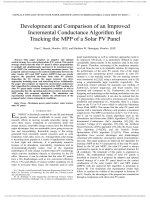
(V×I) is maximum. This point is known as the MPP and is
unique, Fig. 1. It is obvious that two important factors which
have to be taken into account in the electricity generation of a
solar PV panel are the irradiation and temperature. These
factors strongly affect the characteristics of solar PV panels.
Thus, the solar PV panel needs to be perpendicular to sunlight
to maximize the irradiation obtained. Additionally, as a result,
the MPP varies during the day and the solar PV panel is
essential to track the MPP in all conditions to ensure that the

maximum available power is obtained. This problem is
entrusted to the maximum power point tracking (MPPT)
algorithms through searching and determining MPPs in
various conditions. This paper proposes the improved InC
algorithm for searching MPPs which is presented in more
detail in Section III.B.

PMPP

Isc
IMPP

0

Power (W)

Current (A)

A solar PV panel is used for generating electricity. A simple
equivalent circuit model for a solar PV cell consists of a real
diode in parallel with an ideal current source [25]. The
mathematical model of the solar PV cell is given by:
 qV

(1)
I  I sc  I 0  e kT  1





2

Voltage (V)

VMPP

Voc

Fig. 1. Important points in the V-I and V-P characteristics of a solar PV panel

III. CONTROL S TRATEGIES FOR A SOLAR P HOTOVOLTAIC
PANEL
A. Sun Tracking Control
The sun rises from the east and moves across the sky to the
west everyday. In order to increase solar yield and electricity
production from solar PV panels, the idea is to be able to tilt
the solar PV panels in the direction which the sun moves
throughout the year as well as under varying weather
conditions. It can be realized that the more the solar PV panels
can face directly towards the sun, the more power can be
generated. This idea is called a solar tracker (ST) which
orients the solar PV panels towards the sun so that they
harness more sunlight. Considering basic construction
principles and tracking drive approaches for the motion of the
tracker, STs can be divided into open- and closed-loop STs.
In the open-loop tracking control strategy, the tracker does
not actively find the sun's position but instead determines the
position of the sun for a particular site. The tracker receives
the current time, day, month and year and then calculates the

position of the sun without using feedback. The tracker
controls a stepper motor to track the sun's position. It can be
realized that no sensor is used in this control strategy. Thus, it
is normally called an open-loop ST. The sun's position can be
described in terms of its altitude angle, β and its azimuth
angle, s at any time of day which depend on the latitude, the
day number and the time of day, Fig. 2 [25].
The altitude angle, β is given by:
(5)
sin   cos L cos  cos H  sin L sin 
The azimuth angle, s is given by:
cos  sin H
(6)
sin s 
cos 
Additionally, it depends on the hour angle, H, the azimuth
angle, s can be estimated as follows:
tan 
, then s  900 ; otherwise s  900
(7)
If cos H 
tan L
The declination angle,  is given by:
 360
(8)
n  81
  23.45 sin 
 365

where

L: the latitude of the site (degrees);
: the declination angle (degrees);

1949-3029 (c) 2015 IEEE. Personal use is permitted, but republication/redistribution requires IEEE permission. See for more information.


This article has been accepted for publication in a future issue of this journal, but has not been fully edited. Content may change prior to final publication. Citation information: DOI 10.1109/TSTE.2016.2556678, IEEE
Transactions on Sustainable Energy

> REPLACE THIS LINE WITH YOUR PAPER IDENTIFICATION NUMBER (DOUBLE-CLICK HERE TO EDIT) <
n: the number of days since January 1;
H: the hour angle (degrees).

more quickly. Fig. 3 describes the rotating state of the closedloop ST when the sun’s position shifts.
Noon

Sun

Sun

Sunrise

Sun

Sun

E

3

S

East of S: s > 0

β s
Shadow

PV
Sunset
West of S: s < 0

A
Sun

W
Fig. 2. Description of the sun's position

The solar declination angle, , is the angle between the plane
of the equator and a line drawn from the center of the sun to
the center of the earth. The hour angle, H, shows the time of
day with respect to the solar noon. It is the angle between the
planes of the meridian-containing observer and meridian that
touches the earth-sun line. It is zero at solar noon and
increases by 150 every hour since the earth rotates 360 0 in 24
hour. Then, the hour angle is described as follows:
(9)
H  150 t s  12 
where
ts: the solar time in hours. It is a 24-hour clock with 12:00 as
the exact time when the sun is at the highest point in the sky.

The open-loop ST must turn the solar PV panel to the east at
the sunrise time and stop its motion at the sunset time. It is
realized that the altitude angle, β is equal to zero at the sunrise
and sunset moments which is described as follows [25]:
(10)
sin   cos L cos  cos H  sin L sin   0

sin L sin 
  tan L tan 
(11)
cos L cos 
(12)
H   cos 1 tan L tan  
The hour angle, H, is the inverse cosine function which has
positive and negative values. The positive values are used for
the sunrise whereas the negative values are used for the sunset.
Then, the sunrise and sunset times are obtained by converting
the hour angle as follows:
H
(13)
Sunrise _ time  Solar _ noon  0
15
H
(14)
Sunset _ time  Solar _ noon  0
15
On the other hand, the closed-loop ST is based on feedback
control principles. In the closed-loop tracking control strategy,
the search of the sun's position is implemented at any time of
day; light sensors are used and positioned on the solar PV

panel. In order to determine the sun's position, two similar
light sensors are mounted on the solar PV panel. They are
located at the east and west, or south and north, to sense the
light source intensity. There is an opaque object between two
sensors which is to isolate the light from other orientations to
obtain a wide-angle search and to determine the sun's position
cos H  

B

Solar PV panel
Fig. 3. Rotating state of the closed-loop ST

The sensors used are light dependent resistors (LDR) in the
closed-loop ST. The closed-loop ST receives the signals which
are the resistance values of two LDRs, RA and RB respectively.
Then, it makes a comparison between RA and RB as follows.
* If RA=RB, then the solar PV panel will be kept its position.
* If RA≠RB and RAtowards A.
* If RA≠RB and RA>RB, then the solar PV panel will be rotated
towards B.
The sample time is the ∆t for the comparison and
determination of the rotated direction. It is obvious that the
solar tracking systems are a good choice for the solar PV
systems. The comparisons between the open- and closed-loop
STs are shown in Table I. It is easily realized that the openloop ST is simpler, less expensive, more reliable, as well as in
need of less maintenance than the closed-loop ST.
Nevertheless, its performance can be sometimes lower than
that of the closed-loop ST, because the open-loop ST does not

observe the output of the processes that it is controlling. No
feedback signal is required in this ST. While the closed-loop
ST can produce a better tracking efficiency, its feedback
signals tracking the sun's position will be lost when the LDRs
are shaded or the sun is blocked by clouds. Additionally, the
closed-loop ST is rather expensive and more complicated than
the open-loop ST because it requires LDRs placed on the solar
PV panel. A comparison is also performed between the openand closed-loop STs through the experimental designs and
results in the next section.
TABLE I
COMPARISON BETWEEN THE OPEN - AND C LOSED -LOOP ST S
Item
Open-loop
Closed-loop
Simple
Complicated
Structure
No required
LDRs
Extra-hardware
Cheap
Expensive
Cost
No required
Required
Feedback signal
Simple
Complicated
Control

B. MPP Tracking Control
The InC algorithm is reviewed in Part 1 of this section
followed by a description of the improved InC algorithm.
1) InC Algorithm
The principle of the InC algorithm is that the derivative of
the power with respect to the voltage or current becomes zero
at the MPP, the power increases with the voltage in the left

1949-3029 (c) 2015 IEEE. Personal use is permitted, but republication/redistribution requires IEEE permission. See for more information.


This article has been accepted for publication in a future issue of this journal, but has not been fully edited. Content may change prior to final publication. Citation information: DOI 10.1109/TSTE.2016.2556678, IEEE
Transactions on Sustainable Energy

> REPLACE THIS LINE WITH YOUR PAPER IDENTIFICATION NUMBER (DOUBLE-CLICK HERE TO EDIT) <
side of the MPP and the power decreases with the voltage in
the right side of the MPP [26]-[27]. This description can be rewritten in the following simple equations:
dp
 0 at the MPP
(15)
dv
dp
 0 to the left of the MPP
(16)
dv
dp
 0 to the right of the MPP
(17)
dv
where

di
dp d (iv )

 I V
(18)
dv
dv
dv
1 dp I di
(19)
 
V dv V dv
Therefore, the voltage of the PV panels can be adjusted
relative to the MPP voltage by measuring the incremental
conductance, di/dv and the instantaneous conductance, I/V. It
can be realized that the InC algorithm overcomes the
oscillation around the MPP when it is reached. When di/dv=I/V is satisfied, this means that the MPP is reached and the
operating point is remained. Otherwise, the operating point
must be changed, which can be determined using the
relationship between di/dv and -I/V. Furthermore, the equation
(19) shows that:
di
I
dp
 0 : the operating point is to the right
  , then
If
dv
V
dv

of the MPP.
di
I
dp
 0 : the operating point is to the left of
  , then
If
dv
V
dv
the MPP.
Additionally, the InC algorithm can track the MPP in the
case of rapidly changing atmospheric conditions easily,
because this algorithm uses the differential of the operating
point, dp/dv. Basically, the algorithm can move the operating
point towards the MPP under varying atmospheric conditions.
Nevertheless, the InC algorithm has the disadvantage of
requiring a control circuit with an associated higher system
cost. It also requires a fast computation for the incremental
conductance. If the speed of computation is not satisfied under
varying atmospheric conditions, the operating point towards
the MPP cannot be guaranteed. Additionally, the search space
is larger in the InC algorithm. This directly affects the search
performance of the algorithm.
2) Improved InC Algorithm
An improved InC algorithm is proposed in order to
overcome the disadvantages of the InC algorithm.
Firstly, the computation for the differential of the operating
point, dp/dv is simplified by the following approximation:
dp P k   P k  1

(20)

dv V k   V k  1
Secondly, the InC algorithm is combined with the Constant
Voltage (CV) algorithm [28]-[29] for the estimation of the
MPP voltage which can limit the search space for the InC

4

algorithm. Basically, the CV algorithm applies the operating
voltage at the MPP which is linearly proportional to the open
circuit voltage of PV panels with varying atmospheric
conditions. The ratio of VMPP/Voc is commonly used around
76% [30]. Thus, the improved InC algorithm is implemented
to divide the P-V characteristic into three areas referred to as
area 1, area 2 and area 3, where area 1 is from 0 to 70%Voc,
area 2 is from 70%Voc to 80%Voc and area 3 is from 80%Voc to
Voc. Area 2 is the area including the MPP, Fig. 4. It can be
realized that the improved InC algorithm only needs to search
the MPP within area 2, from 70%Voc to 80%Voc. This means
that:
(21)
Vref  70%  80% Voc  V1  V2 
In the improved InC algorithm, the MPPT system
momentarily sets the PV panels current to zero allowing
measurement of the panels' open circuit voltage. The operation
of the improved InC algorithm is shown in the flow chart, Fig.
5. Finally, the ST and MPPT are combined to control the solar
PV panel so that the obtained electricity is maximized under
all atmospheric conditions.

IV. SIMULATION RESULTS
Simulations are performed using MATLAB/SIMULINK
software for tracking MPPs of the solar PV array with 7
panels, RS-P618-22 connected in series whose specifications
and parameters are in Table II. The solar PV panel provides a
maximum output power at a MPP with VMPP and IMPP. The
MPP is defined at the standard test condition (STC) of the
irradiation, 1 kW/m2 and module temperature, 25 0C but this
condition does not exist most of the time. The following
simulations are implemented to confirm the effectiveness of
the improved InC algorithm which is compared with those of
the InC and P&O algorithms.
Case 1: It is assumed that the module temperature is constant,
T=250C. Fig. 6 describes the variation of the solar irradiation
where 0st<1s: G=0.25 kW/m2; 1st<2s: G=0.5kW/m2;
2st<3s: G=0.75kW/m2; 3st<4s: G=1kW/m2 and 4st5s:
G=0.25kW/m2. Then, the obtained output powers are shown as
in Figs. 7-8 using the P&O, InC and improved InC algorithms,
respectively under the various solar irradiations.
Case 2: It is assumed that both the module temperature and
solar irradiation are changed, where the module temperature
variation is as follows: 0st<1s: T=250C; 1st<2s: T=300C;
2st<3s: T=350C; 3st<4s: T=400C; 4st5s: T=250C, Fig. 6
and the solar irradiation variation is as in case 1. Then, the
obtained output powers are shown as in Figs. 9-10 using the
P&O, InC and improved InC algorithms under the variation of
both the temperature and solar irradiation. Figs. 11-12 show
the MPPs of the solar PV panel under the variations of the
solar irradiation and temperature. It can be realized that the
simulation results of the cases using the improved InC

algorithm are always better than the cases using the P&O and
InC algorithms, Figs. 7-8 and Figs. 9-10. The better results are
shown through the algorithm convergence and the MPPs’
tracking ability, especially with the rapid variation of both the
temperature and solar irradiation. This means that the

1949-3029 (c) 2015 IEEE. Personal use is permitted, but republication/redistribution requires IEEE permission. See for more information.


This article has been accepted for publication in a future issue of this journal, but has not been fully edited. Content may change prior to final publication. Citation information: DOI 10.1109/TSTE.2016.2556678, IEEE
Transactions on Sustainable Energy

> REPLACE THIS LINE WITH YOUR PAPER IDENTIFICATION NUMBER (DOUBLE-CLICK HERE TO EDIT) <

TABLE II
SPECIFICATIONS AND PARAMETERS OF THE SOLAR PV PANEL RS-P618-22
Maximum power, P max(W)
22
17.64
Voltage at P max, V MPP(V)
Current at P max, I MPP (A)
1.25
1.34
Short-circuit current, Isc (A)
Open-circuit voltage, Voc (V)
21.99
TABLE III
CONTROL S TRATEGIES FOR A SOLAR PV P ANEL
Strategy
1

2
3
4
5
6
7
  

 

Open-loop ST
  

  
Closed-loop ST
 


  
InC based MPPT
 


  
Improved InC based MPPT
MPP

0

V1

Voltage (V)

Area 3

Area 2

The experimental results are also implemented with the
same solar PV panel, RS-P618-22. In the solar tracking
strategies, a stepper motor is used as the drive source to rotate
the solar PV panel. This motor is run with the output signals
which are received from the LDRs. The block diagram and
setup of the experiment are shown in Figs. 13-14. The
experimental result of obtained maximum output power using
the improved InC algorithm under the variation of the solar
irradiation of the simulation case 1 is shown in Fig. 15. This
experimental result also shows that the output power always
tracks the MPPs. Furthermore, the experiment for the control
strategies, described in Table III of the solar PV panel with the
proposed ST and MPPT algorithms, is also implemented
outdoors from 07:00 AM to 05:00 PM by measuring the
voltage and current for the same load at different times; and
calculating the total power. Table III describes the control
strategies for the solar PV panel as follows.
* Strategy 1: A PV is not controlled by the ST and MPPT.
* Strategy 2: A PV is controlled by the open-loop ST.
* Strategy 3: A PV is controlled by the closed-loop ST.
* Strategy 4: A PV is controlled by the open-loop ST and
the InC algorithm based MPPT.
* Strategy 5: A PV is controlled by the open-loop ST and
the improved InC algorithm based MPPT.

* Strategy 6: A PV is controlled by the closed-loop ST and
the InC algorithm based MPPT.
* Strategy 7: A PV is controlled by the closed-loop ST and
the improved InC algorithm based MPPT.
Table IV shows that the total powers generated by the solar
PV panel are 137.91 W using strategy 1; 173.72 W using
strategy 2 and 183.42 W using strategy 3. It is obvious that the
total power of the solar PV panel using strategy 3 is largest.
The total powers generated by the solar PV panel are 176.35
W using strategy 4; and 188.03 W using strategy 5. It is
obvious that the total power of the solar PV panel using
strategy 5 is larger than that using strategy 4. The total powers
generated by the solar PV panel are 185.86 W using strategy
6; and 197.58 W using strategy 7. It is obvious that the total
power of the solar PV panel using strategy 7 is larger than that
using strategy 6. The comparison of the obtained powers of
the solar PV panel between seven strategies is shown in Fig.
16. Additionally, the improvement percentage of the obtained
powers of the solar PV panel using the control strategies is
shown in Table V. Table V shows that strategies 2-7 with the
ST and MPPT algorithms are better than strategy 1.
Obviously, strategy 7 is the best one with the improvement
percentage, 43.27%. This clearly shows the benefit of the
improved InC algorithm based MPPT when used in
conjunction with the closed-loop ST. Strategy 3 with the
closed-loop ST is better than strategy 2 with the open-loop ST.
However, it can be realized that the structure and operating
principle of the closed-loop ST is more complicated than that
of the open-loop ST and not as reliable, Table I. Additionally,

Area 1

V. EXPERIMENTAL RESULTS

the cost of the closed-loop ST is more expensive. Thus there is
an economic reason not to use it. The comparisons between
strategies 5 and 4; as well as 7 and 6 confirm the effectiveness
of the improved InC algorithm based MPPT strategy.

Power (W)

drawbacks of the InC algorithm have been overcome using the
proposed InC algorithm.

5

V2

Voc

Fig. 4. Area partition of the P-V characteristic
Begin
Determine: V1 and V2
Measure: V(k) and I(k)
Compute: P(k)=V(k)×I(k)

dv=V(k)-V(k-1)
dp=P(k)-P(k-1)
Yes

V(k)No

Yes

V(k)>V2
No
dp/dv=0

Yes

No
dp/dv>0

Yes

No
V(k)+V

V(k)-V

V(k)-V

V(k)+V

Return
Fig. 5. Flow chart of the improved InC algorithm

1949-3029 (c) 2015 IEEE. Personal use is permitted, but republication/redistribution requires IEEE permission. See for more information.

This article has been accepted for publication in a future issue of this journal, but has not been fully edited. Content may change prior to final publication. Citation information: DOI 10.1109/TSTE.2016.2556678, IEEE
Transactions on Sustainable Energy

> REPLACE THIS LINE WITH YOUR PAPER IDENTIFICATION NUMBER (DOUBLE-CLICK HERE TO EDIT) <
50

1 kW/m2

Solar irradiation
0.75 kW/m2

0.7
0.6
0.5

40
35
30

400 C

350 C
0

30 C
250 C

25

250 C

0.5 kW/m2

0.4

20

0.3
2

2

0.25 kW/m

0.25 kW/m

15
10

Obtained maximum power, P(W)

Temperature

0.8

0.2

160

45
Temperature, T(0C)

Solar irradiation, G(kW/m 2)

1
0.9

5

0.1
0
0

1

140
120

60
40
20
0

1

140

100

2

5

60
40
20
0

1

2

3

4



0

0.75 kW/m , 25 C

120

P&O
80



0.5 kW/m2, 250C

100
80

0.25 kW/m2, 250C



60
40

5

T ime, t(s)



20

Fig. 7. Obtained maximum output power with the P&O and improved InC
algorithms under the variation of the solar irradiation

0

160

0

10

20
30
PV Voltage, Vpv (V)

140

40

50

Fig. 11. MPPs of the solar PV panel under the variation of the solar irradiation

120

Improved InC

160

InC

140

1 kW/m2, 400C

100
80

20
0

1

2

3

4

5

Time, t(s)

Fig. 8. Obtained maximum output power with the InC and improved InC
algorithms under the variation of the solar irradiation
160

PV Power, Ppv (W)

40

80

0.25 kW/m2, 250C

60



40



20
0

10

120

Improved InC



0.5 kW/m2, 300C

100

0

140



0.75 kW/m2, 350C

120

60

20
30
PV Voltage, Vpv (V)

40

50

Fig. 12. MPPs of the solar PV panel under both the variations of the solar
irradiation and temperature

100

P&O

80

Sun

60

DC

40

Load

PV
DC

20
0

4

1 kW/m2, 250C

140

Improved InC

0

3

160

120

0

2
Time, t(s)

PV Power, Ppv (W)

Obtained maximum power, P (W)

0

Fig. 10. Obtained maximum output power with the InC and improved InC
algorithms under both the variations of the solar irradiation and temperature

160

Obtained maximum power, P(W)

InC

80

3
4
5
Time, t(s)
Fig. 6. Description of the variations of the solar irradiation and temperature

Obtained maximum power, P(W)

Improved InC

100

0

2

6

ipv

0

1

2

3

4

5

vpv

T ime, t(s)

Fig. 9. Obtained maximum output power with the P&O and improved InC
algorithms under both the variations of the solar irradiation and temperature

Stepper
motor

MPPT
ST

Fig. 13. Block diagram of the experimental setup

1949-3029 (c) 2015 IEEE. Personal use is permitted, but republication/redistribution requires IEEE permission. See for more information.

This article has been accepted for publication in a future issue of this journal, but has not been fully edited. Content may change prior to final publication. Citation information: DOI 10.1109/TSTE.2016.2556678, IEEE
Transactions on Sustainable Energy

> REPLACE THIS LINE WITH YOUR PAPER IDENTIFICATION NUMBER (DOUBLE-CLICK HERE TO EDIT) <

7

proposed adaptive and optimal control strategy in the solar PV
panel through the comparisons with other strategies.
REFERENCES
[1]
[2]

[3]

[4]

Fig. 14. Experimental setup

[5]

[6]

[7]

[8]

[9]

[10]

Fig. 15. Experimental result of obtained maximum output power with the
improved InC algorithm under the variation of the solar irradiation

[11]

250

[12]

Power (W)

200

150

[13]

100

[14]

50

0
Strategy 1 Strategy 2 Strategy 3 Strategy 4 Strategy 5 Strategy 6 Strategy 7

[15]

Fig. 16. Comparison of the obtained powers of the solar PV panel between
strategies 1-7

[16]

VI. CONCLUSION

[17]

It is obvious that the adaptive and optimal control strategy
plays an important role in the development of solar PV
systems. This strategy is based on the combination between
the ST and MPPT in order to ensure that the solar PV panel is
capable of harnessing the maximum solar energy following
the sun's trajectory from dawn until dusk and is always
operated at the MPPs with the improved InC algorithm. The
proposed InC algorithm improves the conventional InC
algorithm with an approximation which reduces the
computational burden as well as the application of the CV
algorithm to limit the search space and increase the
convergence speed of the InC algorithm. This improvement
overcomes the existing drawbacks of the InC algorithm. The
simulation and experimental results confirm the validity of the

[18]

[19]

[20]

[21]

[22]

R. Faranda and S. Leva, “Energy comparison of MPPT techniques for
PV systems,” Trans. Power Syst., vol. 3, no. 6, pp. 446-455, 2008.
X. Jun-Ming, J. Ling-Yun, Z. Hai-Ming and Z. Rui, “Design of track
control system in PV,” IEEE Int. Conf. Software Engineering and
Service Sciences, ICSESS2010, pp. 547-550, 2010.
Z. Bao-Jian, G. Guo-Hong and Z. Yan-Li, “Designment of automatic
tracking system of solar energy system,” 2nd Int. Conf. Industrial
Mechatronics and Automation, ICIMA2010, pp. 689-691, 2010.
W. Luo, “A solar panels automatic tracking system based on OMRON
PLC,” Proc. 7th Asian Control Conf., pp. 1611-1614, 2009.
W. Chun-Sheng, W. Yi-Bo, L. Si-Yang, P. Yan-Chang and X. HongHua, “Study on automatic sun-tracking technology in PV generation,”
Third Int. Conf. Electric Utility Deregulation and Restructuring and
Power Technologies, DRPT2008, pp. 2586-2591, 2008.
C. Alexandru and C. Pozna, “Different tracking strategies for optimizing
the energetic efficiency of a photovoltaic system,” Int. Conf.
Automation, Quality and Testing, Robotics, pp. 434-439, 2008.
R. Sridhar, S. Jeevananthan, N. T. Selvan and P. V. SujithChowdary,
“Performance improvement of a photovoltaic array using MPPT P&O
technique,” Int. Conf. Control and Comput. Technol., pp. 191-195, 2010.
N. M. Razali and N. A. Rahim, “DSP-based maximum peak power
tracker using P&O algorithm,” IEEE First Conf. Clean Energy and
Technol., pp. 34-39, 2011.
L. Chun-Xia, L. Li-qun, “An improved perturbation and observation
MPPT method of photovoltaic generate system,” 4th IEEE Conf. Ind.
Electron. and Appl., ICIEA2009, pp. 2966-2970, 2009
Y. Jung, J. So, G. Yu and J. Choi, “Improved perturbation and
observation method (IP&O) of MPPT control for photovoltaic power
systems,” 31st IEEE Photov. Specialists Conf., pp. 1788-1791, 2005.

X. Liu, L. A. C. Lopes, “An improved perturbation and observation
maximum power point tracking algorithm for PV arrays,” IEEE 35th
Annual Power Electron. Specialists Conf., pp. 2005-2010, 2004.
D. C. Huynh, T. A. T. Nguyen, M. W. Dunnigan and M. A. Mueller,
“Maximum power point tracking of solar photovoltaic panels using
advanced perturbation and observation algorithm,” IEEE Conf.
Industrial Electronics and Applications 2013, pp. 864-869, 2013.
B. Liu, S. Duan, F. Liu and P. Xu, “Analysis and improvement of
maximum power point tracking algorithm based on incremental
conductance method for photovoltaic array,” 7th Int. Conf. Power
Electron. and Drive Syst., PEDS2007, pp. 637-641, 2007.
W. Ping, D. Hui, D. Changyu and Q. Shengbiao, “An improved MPPT
algorithm based on traditional incremental conductance method,” 4th
Int. Conf. Power Electron. Syst. and Appl, PESA2011, pp. 1-4, 2011.
Y. Zhihao and W. Xiaobo, “Compensation loop design of a photovoltaic
system based on constant voltage MPPT,” Asia-Pacific Power and
Energy Eng. Conf., APPEEC2009, pp. 1-4, 2009.
K. A. Aganah and A. W. Leedy, “A constant voltage maximum power
point tracking method for solar powered systems,” IEEE 43rd
Southeastern Sym. Syst. Theory, SSST2011, pp. 125-130, 2011.
P. Q. Dzung, L. D. Khoa, H. H. Lee, L. M. Phuong and N. T. D. Vu,
“The new MPPT algorithm using ANN based PV,” Int. Forum on
Strategic Technology, IFOST2010, pp. 402-407, 2010.
R. Ramaprabha, V. Gothandaraman, K. Kanimozhi, R. Divya and B. L.
Mathur, “Maximum power point tracking using GA-optimized artificial
neural network for solar PV system,” 1st Int. Conf. Electr. Energy Syst.,
ICEES2011, pp. 264-268, 2011.
S. J. Kang, J. S. Ko, J. S. Choi, M. G. Jang, J. H. Mun, J. G. Lee and D.
H. Chung, “A novel MPPT control of photovoltaic system using FLC
algorithm,” 11th Int. Conf. Contr., Autom. and Syst., pp. 434-439. 2011.

V. Padmanabhan, V. Beena and M. Jayaraju, “Fuzzy logic based
maximum power point tracker for a photovoltaic system,” Int. Conf.
Power, Signals, Contr. and Comput., EPSCICON2012, pp. 1-6, 2012.
Md. A. Azam, S. A. A. Nahid, M. M. Alam and B. A. Plabon,
“Microcontroller based high precision PSO algorithm for maximum
solar power tracking,” Conf. Electron. and Vision, pp. 292-297, 2012.
K. Ishaque, Z. Salam, M. Amjad and S. Mekhilef, “An improved particle
swarm optimization (PSO)-based MPPT for PV with reduced steadystate oscillation,” IEEE Trans. Power Electron., pp. 3627-3638, 2012.

1949-3029 (c) 2015 IEEE. Personal use is permitted, but republication/redistribution requires IEEE permission. See for more information.


This article has been accepted for publication in a future issue of this journal, but has not been fully edited. Content may change prior to final publication. Citation information: DOI 10.1109/TSTE.2016.2556678, IEEE
Transactions on Sustainable Energy

> REPLACE THIS LINE WITH YOUR PAPER IDENTIFICATION NUMBER (DOUBLE-CLICK HERE TO EDIT) <
[23] D. C. Huynh, T. N. Nguyen, M. W. Dunnigan and M. A. Mueller,
“Dynamic particle swarm optimization algorithm based maximum
power point tracking of solar photovoltaic panels,” IEEE International
Symp. Industrial Electronics 2013, ISIE2013, pp. 1-6, 2013.
[24] D. C. Huynh, T. M. Nguyen, M. W. Dunnigan and M. A. Mueller,
“Global MPPT of solar PV modules using a dynamic PSO algorithm
under partial shading conditions,” IEEE Int. Conf. Clean Energy &
Technology 2013, CEAT2013, pp. 133-138, 2013.
[25] G. M. Master, “Renewable and efficient electric power systems,” in
Renewable and efficient electric power systems, A John Wiley & Sons,
Inc., Publication, pp. 385-604, 2004.
[26] B. Liu, S. Duan, F. Liu and P. Xu, “Analysis and improvement of
maximum power point tracking algorithm based on incremental
conductance method for photovoltaic array,” 7th Int. Conf. Power

Electron. and Drive Syst., PEDS2007, pp. 637-641, 2007.
[27] W. Ping, D. Hui, D. Changyu and Q. Shengbiao, “An improved MPPT
algorithm based on traditional incremental conductance method,” 4th
Int. Conf. Power Electron. Syst. and Appl, PESA2011, pp. 1-4, 2011.
[28] Y. Zhihao and W. Xiaobo, “Compensation loop design of a photovoltaic
system based on constant voltage MPPT,” Asia-Pacific Power and
Energy Eng. Conf., APPEEC2009, pp. 1-4, 2009.
[29] K. A. Aganah and A. W. Leedy, “A constant voltage maximum power
point tracking method for solar powered systems,” IEEE 43rd
Southeastern Sym. Syst. Theory, SSST2011, pp. 125-130, 2011.
[30] J. H. R. Enslin, M. S. Wolf, D. B. Snyman and W. Sweigers, “Integrated
photovoltaic maximum power point tracking converter,” IEEE Trans.
Ind. Elec., vol. 44, no. 6, pp. 769-773, 1997.

Duy C. Huynh received the B.Sc. and
M.Sc. degrees in electrical and
electronic engineering from Ho Chi
Minh City University of Technology,
Ho Chi Minh City, Vietnam, in 2001
and 2005, respectively and Ph.D.
degree from Heriot-Watt University,
Edinburgh, U.K., in 2010. In 2001, he

Time
07:00 AM
07:30 AM
08:00 AM
08:30 AM
09:00 AM
09:30 AM

10:00 AM
10:30 AM
11:00 AM
11:30 AM
12:00 PM
12:30 PM
01:00 PM
01:30 PM
02:00 PM
02:30 PM
03:00 PM
03:30 PM
04:00 PM
04:30 PM
05:00 PM
Total

8

became a Lecturer at Ho Chi Minh City University of
Technology. His research interests include the areas of energy
efficient control and parameter estimation methods of
induction machines and renewable sources.
Matthew W. Dunnigan received his
B.Sc. in Electrical and Electronic
Engineering (with First-Class Honours)
from Glasgow University, Glasgow,
U.K., in 1985 and his M.Sc. and Ph.D.
from
Heriot-Watt

University,
Edinburgh, UK, in 1989 and 1994,
respectively. He was employed by
Ferranti from 1985 to 1988 as a
Development Engineer in the design of
power supplies and control systems for moving optical
assemblies and device temperature stabilisation. In 1989, he
became a Lecturer at Heriot-Watt University, where he was
concerned with the evaluation and reduction of the dynamic
coupling between a robotic manipulator and an underwater
vehicle. He is currently a Senior Lecturer, Associate Professor
and his research grants and interests include the areas of
hybrid position/force control of an underwater manipulator,
coupled control of manipulator-vehicle systems, nonlinear
position/speed control and parameter estimation methods in
vector control of induction machines, frequency domain selftuning/adaptive filter control methods for random vibration,
and shock testing using electro-dynamic actuators.

TABLE IV
COMPARISON OF THE OBTAINED POWERS OF THE SOLAR PV P ANEL BETWEEN STRATEGIES 1-7
PStrategy1 (W)
PStrategy5 (W)
PStrategy6 (W)
PStrategy2 (W)
PStrategy3 (W)
PStrategy4 (W)
0.16
0.48
0.72
0.51

0.54
0.76
0.74
1.51
1.98
1.61
1.72
2.01
0.76
3.14
3.25
3.50
3.57
3.29
1.06
3.60
3.80
4.06
4.10
4.21
3.30
5.19
5.23
5.23
5.92
5.18
4.76
7.85
8.84
8.22

8.94
9.38
11.48
12.86
13.26
13.05
13.75
13.04
11.04
13.34
13.35
13.49
14.26
13.62
12.43
13.92
13.78
14.30
14.89
13.96
12.84
14.66
14.79
14.96
15.68
14.94
13.07
15.98
16.17
16.21

16.65
16.54
13.53
15.58
15.95
16.18
16.23
16.17
13.13
14.90
15.44
15.40
16.19
15.45
10.19
11.10
11.42
10.87
12.06
11.12
6.57
7.27
8.48
7.36
7.90
8.41
5.58
9.19
10.18
8.76

9.98
10.58
5.01
6.70
7.64
6.40
7.28
7.75
4.37
5.60
5.70
5.36
6.25
5.73
3.15
4.22
5.21
4.14
4.71
5.21
2.84
3.66
4.28
3.51
4.08
4.47
1.89
2.98
3.94
3.23

3.32
4.03
137.91
173.72
183.42
176.35
188.03
185.86

PStrategy7 (W)
0.8
2.21
3.63
4.33
5.96
10.08
14.00
14.10
14.55
15.62
17.08
16.83
16.31
12.13
9.00
11.50
8.62
6.20
5.67
4.66

4.28
197.58

TABLE V
IMPROVEMENT P ERCENTAGE OF THE OBTAINED POWERS OF THE SOLAR PV PANEL USING THE VARIOUS CONTROL STRATEGIES
Comparison
Strategies Strategies Strategies Strategies Strategies Strategies Strategies Strategies Strategies
between strategies
2 and 1
3 and 1
4 and 1
5 and 1
6 and 1
7 and 1
3 and 2
5 and 4
7 and 6
25.97
33.00
27.87
36.34
34.77
43.27
5.58
6.62
6.31
Improvement (%)

1949-3029 (c) 2015 IEEE. Personal use is permitted, but republication/redistribution requires IEEE permission. See for more information.