DSpace at VNU: Prescribing Webster scalar curvature on CR manifolds of negative conformal invariants
Bạn đang xem bản rút gọn của tài liệu. Xem và tải ngay bản đầy đủ của tài liệu tại đây (1.82 MB, 48 trang )
JID:YJDEQ AID:7737 /FLA
[m1+; v1.204; Prn:12/03/2015; 14:29] P.1 (1-48)
Available online at www.sciencedirect.com
ScienceDirect
J. Differential Equations ••• (••••) •••–•••
www.elsevier.com/locate/jde
Prescribing Webster scalar curvature on CR manifolds
of negative conformal invariants
´ Anh Ngô a , Hong Zhang b,∗,1
Quôc
a Department of Mathematics, College of Science, Viêt Nam National University, Hà Nôi, Viet Nam
b Department of Mathematics, National University of Singapore, Block S17, 10 Lower Kent Ridge Road,
Singapore 119076, Singapore
Received 19 October 2014
Abstract
In this paper, we are interested in solving the following partial differential equation
− θ u + Ru = f u1+2/n
on a compact strictly pseudo-convex CR manifold (M, θ) of dimension 2n + 1 with n 1. This problem
naturally arises when solving the prescribing Webster scalar curvature problem on M with the prescribed
function f . Using variational techniques, we prove several non-existence, existence, and multiplicity results
when the function f is sign-changing.
© 2015 Elsevier Inc. All rights reserved.
MSC: primary 32V20, 35H20; secondary 58E05
Keywords: Prescribed Webster scalar curvature; Negative conformal invariant; Compact CR manifolds; Critical
exponent; Variational methods
* Corresponding author.
E-mail addresses: (Q.A. Ngô), ,
(H. Zhang).
1 Current address: Center for PDE, East China Normal University, Shanghai 200241, China.
/>0022-0396/© 2015 Elsevier Inc. All rights reserved.
JID:YJDEQ AID:7737 /FLA
[m1+; v1.204; Prn:12/03/2015; 14:29] P.2 (1-48)
Q.A. Ngô, H. Zhang / J. Differential Equations ••• (••••) •••–•••
2
Contents
1.
2.
Introduction . . . . . . . . . . . . . . . . . . . . . . . . . . . . . . . . . . . . .
Notations and necessary conditions . . . . . . . . . . . . . . . . . . . . . .
2.1. A necessary condition for f . . . . . . . . . . . . . . . . . . . . . .
2.2. A necessary condition for R . . . . . . . . . . . . . . . . . . . . . .
3. The analysis of the energy functionals . . . . . . . . . . . . . . . . . . . .
3.1. μk,q is achieved . . . . . . . . . . . . . . . . . . . . . . . . . . . . . .
3.2. Asymptotic behavior of μk,q . . . . . . . . . . . . . . . . . . . . .
3.3. The study of λf,η,q . . . . . . . . . . . . . . . . . . . . . . . . . . . .
3.4. μk,q > 0 for some k . . . . . . . . . . . . . . . . . . . . . . . . . . .
3.5. The Palais–Smale condition . . . . . . . . . . . . . . . . . . . . . .
4. Proof of Theorem 1.1(a)–(b) . . . . . . . . . . . . . . . . . . . . . . . . . .
4.1. The existence of the first solution . . . . . . . . . . . . . . . . . .
4.2. The existence of the second solution . . . . . . . . . . . . . . . .
5. Proof of Theorems 1.2, 1.3, and 1.1(c) . . . . . . . . . . . . . . . . . . . .
5.1. Proof of Theorem 1.2 . . . . . . . . . . . . . . . . . . . . . . . . . .
5.2. Proof of Theorem 1.3 . . . . . . . . . . . . . . . . . . . . . . . . . .
5.3. Proof of Theorem 1.1(c) . . . . . . . . . . . . . . . . . . . . . . . .
Acknowledgments . . . . . . . . . . . . . . . . . . . . . . . . . . . . . . . . . . . . . .
Appendix A. Construction of a function satisfying (1.7) and (1.8) . . .
Appendix B. Solvability of the equation − θ u = f . . . . . . . . . . . . .
Appendix C. The method of sub- and super-solutions on CR manifolds
References . . . . . . . . . . . . . . . . . . . . . . . . . . . . . . . . . . . . . . . . . . .
.
.
.
.
.
.
.
.
.
.
.
.
.
.
.
.
.
.
.
.
.
.
.
.
.
.
.
.
.
.
.
.
.
.
.
.
.
.
.
.
.
.
.
.
.
.
.
.
.
.
.
.
.
.
.
.
.
.
.
.
.
.
.
.
.
.
.
.
.
.
.
.
.
.
.
.
.
.
.
.
.
.
.
.
.
.
.
.
.
.
.
.
.
.
.
.
.
.
.
.
.
.
.
.
.
.
.
.
.
.
..
..
..
..
..
..
..
..
..
..
..
..
..
..
..
..
..
..
..
..
..
..
.............
.............
.............
.............
.............
.............
.............
.............
.............
.............
.............
.............
.............
.............
.............
.............
.............
.............
.............
.............
.............
.............
2
6
8
8
10
10
11
15
19
22
25
25
28
36
36
38
39
42
42
43
44
47
1. Introduction
The problem of finding a conformal metric on a manifold with certain prescribed curvature
function has been extensively studied during the last few decades. A typical model is the prescribing scalar curvature problem on closed Riemannian manifolds (i.e. compact without boundary).
More precisely, let (M, g) be an n-dimensional closed manifold with n 3. A conformal change
of metrics, say g = u4/(n−2) g, of the background metric g admits the following scalar curvature
n+2
Scalg = u− n−2 −
4(n − 1)
n−2
g u + Scalg u
where g = div(∇) is the Laplace–Beltrami operator with respect to the metric g and Scalg is
the scalar curvature of the metric g. For a given smooth function f , it is immediately to see
that the problem of solving Scalg = f is equivalent to solving the following partial differential
equation
−
4(n − 1)
n−2
n+2
g u + Scalg u = f u n−2
on M
(1.1)
for u > 0. Clearly, this problem includes the well-known Yamabe problem as a special case when
the candidate function f is constant. While the Yamabe problem had already been settled down
by a series of seminal works due to Yamabe, Trudinger, Aubin, and Schoen, Eq. (1.1) in its
generic form remains open, see [1]. Since Eq. (1.1) is conformal invariant, when solving (1.1),
one often uses the so-called Yamabe invariant to characterize the catalogue of possible metrics
JID:YJDEQ AID:7737 /FLA
[m1+; v1.204; Prn:12/03/2015; 14:29] P.3 (1-48)
Q.A. Ngô, H. Zhang / J. Differential Equations ••• (••••) •••–•••
3
g which eventually helps us to fix a sign for Scalg which depends on the sign of the Yamabe
invariant.
While the case of positive Yamabe invariants remains less understood especially when (M, g)
is the standard sphere (Sn , gSn ), more or less the case of non-positive Yamabe invariants is wellunderstood by a series of works due to Kadzan–Warner, Ouyang, Rauzy, see [29–31] and the
references therein. Intuitively, when the background metric g is of negative Yamabe invariant,
i.e. Scalg < 0, the condition M f dvg < 0 is necessary. Clearly, the most interesting case in this
catalogue is the case when f changes sign and M f dvg < 0. In literature, there are two different
routes that have been used to solve (1.1). The first set of works is based on the geometric implementation of the problem where one fixes Scalg and tries to find conditions for the candidate f ,
for example a work by Rauzy [31]. In [31], it was proved by variational techniques that when
the set {x ∈ M : f (x) 0} has positive measure, Scalg cannot be too negative. In fact, | Scalg | is
bounded from above by some number λf , depending only on the set {x ∈ M : f (x) 0}, which
can be characterized by the following variational problem
⎧
⎪
⎨ inf
λf = u∈A
⎪
⎩
+∞,
M
|∇u|2g dμg
M
u2 dμg
,
if A = ∅,
(1.2)
if A = ∅,
here f ± = max{±f, 0} and
A = u ∈ H 1 (M) : u
|f − |u dμg = 0 .
0, u ≡ 0,
M
In addition, it was proved in [31] that if supM f + is small enough compared with f − , Eq. (1.1)
admits at least one positive smooth solution. In the second route, one can free (1.1) from geometry and fix f instead of Scalg , for example two works by Ouyang [29,30]. In these works, using
bifurcation method, Ouyang proved, among other things, that depending on how small | Scalg |
is Eq. (1.1) always admits either one or two positive smooth solutions. As far as we know, this is
the first multiplicity result for (1.1) when Scalg < 0.
As a natural analogue of the prescribed scalar curvature problem for the CR geometry, one
can consider the prescribed Webster (pseudo-hermitian) scalar curvature problem on compact CR
manifolds which can be formulated as follows. Let (M, θ ) be a compact strictly pseudo-convex
CR manifold without boundary of real dimension 2n + 1 with n 1. Given any smooth function
h on M, it is natural to ask: Does there exist a contact form θ conformally related to θ in the
sense that θ = u2/n θ for some smooth function u > 0 such that h is the Webster scalar curvature
of the Webster metric gθ associated with the contact form θ ? Following the same way as in the
Riemannian case, the Webster metric gθ associated with θ obeys its scalar curvature which is
given by
Scalθ = u−
n+2
n
−
2(n + 1)
n
θ u + Scalθ
u ,
where θ is the sub-Laplacian with respect to the contact form θ , and Scalθ is the Webster scalar
curvature of the Webster metric gθ associated with the contact form θ . Clearly, the problem of
solving Scalθ = h is equivalent to finding positive solutions u to the following PDE
JID:YJDEQ AID:7737 /FLA
4
[m1+; v1.204; Prn:12/03/2015; 14:29] P.4 (1-48)
Q.A. Ngô, H. Zhang / J. Differential Equations ••• (••••) •••–•••
−
θu +
n
n
Scalθ u =
hu1+2/n
2(n + 1)
2(n + 1)
on M.
(1.3)
When h is constant, Eq. (1.3) is known as the CR Yamabe problem. In a series of seminal papers
[16–18], Jerison and Lee extensively studied the Yamabe problem on CR manifolds. As always,
the works by Jerison and Lee also depend on the sign of following invariant
μ(M, θ) =
inf
M
(2 + 2/n)|∇θ u|2θ + Scalθ u2 θ ∧ (dθ )n
2+2/n θ ∧ (dθ )n
M |u|
u∈S21 (M),u≡0
n/(n+1)
,
where S21 (M) is the Folland–Stein space, see Section 2 below. Later on, Gamara and Yacoub
[13,14] treated the cases left open by Jerison and Lee. On the contrary, to the best of authors’
knowledge, only very few results have been established on the prescribed Webster scalar curvature problem, see [9,11,15,23,32], in spit of the vary existing results on its Riemannian analogue,
see [2–8,20–22,28] and the references therein. Among them, Refs. [23] and [32] considered the
prescribing Webster scalar problem on CR spheres; Ho [15] showed, via a flow method, that Eq.
(1.3) has a smooth positive solution if both the Webster scalar curvature Scalθ and the candidate
function h are strictly negative.
The primary aim of the paper is to carry the Rauzy and Ouyang results from the context of
Riemannian geometry to CR geometry. As such, in this article, we investigate the prescribing
Webster scalar curvature problem (1.3) on compact CR manifolds with negative conformal invariants, that is to say μ(M, θ ) < 0. To study (1.3), we mainly follow the Rauzy variational
method in [31] plus some modification taken from a recent paper by the first author together
with Xu in [25], see also [24,26,27]. Loosely speaking, in [25], they proved some existence and
multiplicity results of the Einstein-scalar field Lichnerowicz equations on closed Riemannian
manifolds which includes (1.1) as a special case.
Before stating our main results and for the sake of simplicity, let us denote R = n Scalθ /
(2n + 2) and f = nh/(2n + 2). Then we can rewrite (1.3) as follows
−
θ u + Ru = f u
1+2/n
on M.
(1.4)
Our main results are included in the three theorems below. First, we obtain the following existence result when f changes sign.
Theorem 1.1. Let (M, θ ) be a compact strictly pseudo-convex CR manifold with a negative
conformal invariant of dimension 2n + 1 with n 1. Suppose that f is smooth function on M
satisfying M f θ ∧ (dθ )n < 0, supM f > 0, and |R| < λf , where λf is given in (2.1) below.
Then:
(a) There exists a constant C1 > 0 depending only on f − which is given by (4.1) below such that
if
⎛
⎞−1
(sup f + ) ⎝
M
|f − | θ ∧ (dθ )n ⎠
< C1 ,
M
then Eq. (1.4) possesses at least one smooth positive solution; and
(1.5)
JID:YJDEQ AID:7737 /FLA
[m1+; v1.204; Prn:12/03/2015; 14:29] P.5 (1-48)
Q.A. Ngô, H. Zhang / J. Differential Equations ••• (••••) •••–•••
5
(b) if we suppose further that
⎛
⎞−1
(sup f + )⎝
M
f
N
θ ∧ (dθ )n ⎠
< C2 ,
(1.6)
M
and that
f
N
θ ∧ (dθ )n > 0
(1.7)
M
for some smooth positive function in M and some positive constant C2 , given in (4.11)
below, depending on , then Eq. (1.4) possesses at least two smooth positive solutions. In
addition, if the function satisfies
∇θ
2
2
−2
N
n
,
n+1
(1.8)
and
1 then the constant C2 is independent of .
N
(c) However, for given f , the condition |R| < λf is not sufficient for the solvability of (1.4) in
the following sense: Given any smooth function f and constant R < 0 with supM f > 0,
n
M f θ ∧ (dθ ) < 0, and |R| < λf , there exists a new continuous function h such that
supM h > 0, M h θ ∧ (dθ )n < 0, and λh > λf but Eq. (1.4) with f replaced by h has no
solution.
Then, in the next result, we focus our attention on the case when f 0. Although the condition |R| < λf is not sufficient in the case supM f > 0, nevertheless, in the case supM f = 0, we
are able to show that |R| < λf is sufficient, thus obtaining necessary and sufficient conditions
for the solvability of (1.4). To be exact, we shall prove the following theorem.
Theorem 1.2. Let (M, θ ) be a compact strictly pseudo-convex CR manifold with a negative
conformal invariant of dimension 2n + 1 with n 1. Suppose that f is a smooth non-positive
function on M such that the set {x ∈ M : f (x) = 0} has positive measure. Then Eq. (1.4) has a
unique smooth positive solution if and only if |R| < λf .
Finally, we show that once the function f having supM f > 0 and M f θ ∧ (dθ )n < 0 is
fixed and if |R| is sufficiently small, then Eq. (1.4) always has positive smooth solutions. The
following theorem is the content of this conclusion.
Theorem 1.3. Let (M, θ ) be a compact strictly pseudo-convex CR manifold with a negative
conformal invariant of dimension 2n + 1 with n 1. Suppose that f is smooth function on M
satisfying M f θ ∧ (dθ )n < 0, supM f > 0. Then, there exists a positive constant C3 given in
(5.4) below such that if |R| < C3 , there Eq. (1.4) admits at least one smooth positive solution.
Let us now briefly mention the organization of the paper. Section 2 consists of preliminaries
and notation. Also in this section, two necessary conditions for the solvability of Eq. (1.4) are also
derived. In Section 3, we perform a careful analysis for the energy functional associated to (1.4).
JID:YJDEQ AID:7737 /FLA
6
[m1+; v1.204; Prn:12/03/2015; 14:29] P.6 (1-48)
Q.A. Ngô, H. Zhang / J. Differential Equations ••• (••••) •••–•••
Having all these preparation, we prove Theorem 1.1(a)–(b) in Section 4 while Theorems 1.2,
1.3, and 1.1(c) will be proved in Section 5. Finally, we put some basic and useful results in
Appendices A, B, and C.
2. Notations and necessary conditions
To start this section, we first collect some well-known facts from CR geometry, for interested
reader, we refer to [10].
As mentioned earlier, by M we mean an orientable CR manifold without boundary of CR
dimension n. This is also equivalent to saying that M is an orientable differentiable manifold
of real dimension 2n + 1 endowed with a pair (H (M), J ) where H (M) is a subbundle of the
tangent bundle T (M) of real rank 2n and J is an integrable complex structure on H (M). Since
M is orientable, there exists a 1-form θ called pseudo-Hermitian structure on M. Then, we can
associate each structure θ to a bilinear form Gθ , called Levi form, which is defined only on
H (M) by
Gθ (X, Y ) = −(dθ )(J X, Y )
∀X, Y ∈ H (M).
Since Gθ is symmetric and J -invariant, we then call (M, θ ) strictly pseudo-convex CR manifold
if the Levi form Gθ associated with the structure θ is positive definite. The structure θ is then a
contact form which immediately induces on M the volume form θ ∧ (dθ )n .
Moreover, θ on a strictly pseudo-convex CR manifold (M, θ ) also determines a “normal”
vector field T on M, called the Reeb vector field of θ . Via the Reeb vector field T , one can extend
the Levi form Gθ on H (M) to a semi-Riemannian metric gθ on T (M), called the Webster metric
of (M, θ ). Let
πH : T (M) → H (M)
be the projection associated to the direct sum T (M) = H (M) ⊕ RT . Now, with the structure θ ,
we can construct a unique affine connection ∇, called the Tanaka–Webster connection on T (M).
Using ∇ and πH , we can define the “horizontal” gradient ∇θ by
∇θ u = πH ∇u.
Again, using the connection ∇ and the projection πH , one can define the sub-Laplacian
acting on a C 2 -function u via
θ
θ u = div(πH ∇u).
Here ∇u is the ordinary gradient of u with respect to gθ which can be written as gθ (∇u, X) =
X(u) for any X. Then integration by parts gives
(
M
θ u)f
θ ∧ (dθ )n = −
∇θ u, ∇θ f
M
θ
θ ∧ (dθ )n
JID:YJDEQ AID:7737 /FLA
[m1+; v1.204; Prn:12/03/2015; 14:29] P.7 (1-48)
Q.A. Ngô, H. Zhang / J. Differential Equations ••• (••••) •••–•••
7
for any smooth function f . In the preceding formula, , θ denotes the inner product via the Levi
form Gθ (or the Webster metric gθ since both ∇θ u and ∇θ v are horizontal). When u ≡ v, we
sometimes simply write |∇θ u|2 instead of ∇θ u, ∇θ u θ .
Having ∇ and gθ in hand, one can talk about the curvature theory such as the curvature tensor
fields, the pseudo-Hermitian Ricci and scalar curvature. Having all these, we denote by Scalθ the
pseudo-Hermitian scalar curvature associated with the Webster metric gθ and the connection ∇,
called the Webster scalar curvature, see [10, Proposition 2.9]. At the very beginning, since we
assume μ(M, θ ) < 0, we may further assume without loss of generality that Scalθ is a negative
constant and that
vol(M, θ ) =
θ ∧ (dθ )n = 1
M
since there always exists such a metric in the conformal class of θ . In particular, R < 0 is constant.
In the context of CR manifolds, instead of using the standard Sobolev space H 1 (M), we find
solutions of (1.4) in the so-called Folland–Stein space S21 (M) which is the completion of C ∞ (M)
with respect to the norm
⎛
⎞1/2
u =⎝
|u|2 θ ∧ (dθ )n ⎠
|∇θ u|2 θ ∧ (dθ )n +
M
.
M
For notational simplicity, we simply denote by
·
p
·
and
S21 (M)
the norms in Lp (M) and
S21 (M) respectively. Besides, the following dimensional constants
2
N =2+ ,
n
2 =2+
1
n
will also be used in the rest of the paper. Suppose that f is a smooth function on M and as before
by f ± we mean f − = inf(f, 0) and f + = sup(f, 0). Similar to (1.2), we also define
⎧
⎪
⎨ inf
λf = u∈A
⎪
⎩
+∞,
M
|∇θ u|2 θ ∧ (dθ )n
,
2
n
M u θ ∧ (dθ )
if A = ∅,
(2.1)
if A = ∅,
where the set A is now given as follows
A = u ∈ S21 (M) : u
|f − |u θ ∧ (dθ )n = 0 .
0, u ≡ 0,
M
Since we are interested in the critical case, throughout this paper, we always assume q ∈ (2 , N ).
Moreover, we will use the following Sobolev inequality
u
2
N
K1 ∇u
2
2
+ A1 u 22 .
(2.2)
JID:YJDEQ AID:7737 /FLA
[m1+; v1.204; Prn:12/03/2015; 14:29] P.8 (1-48)
Q.A. Ngô, H. Zhang / J. Differential Equations ••• (••••) •••–•••
8
If we denote C = K1 + A1 , then we obtain from (2.2) the following simpler Sobolev inequality
u
2
N
C u
2
.
S21 (M)
(2.3)
Notice that K1 may not be the best Sobolev constant for the embedding S21 (M) → LN (M). If
the manifold is the Heisenberg group or CR spheres, then the best constant has been found by
Jerison and Lee in [18] (see also [12]). However, for generic CR manifolds, we have not seen
any proof of the best Sobolev constant. Hence, in the present paper, it is safe to use the inequality
(2.3).
2.1. A necessary condition for f
The aim of this subsection is to derive a necessary condition for f so that Eq. (1.4) admits a
positive smooth solution.
Proposition 2.1. Suppose that Eq. (1.4) has a positive smooth solution then
M
f θ ∧ (dθ )n < 0.
Proof. Assume that u > 0 is a smooth solution of (1.4). By multiplying both sides of (1.4) by
u1−N , integrating over M and the fact that R < 0, we obtain
(−
1−N
θ u)u
θ ∧ (dθ )n >
M
f θ ∧ (dθ )n .
M
It follows from the divergence theorem that
(−
1−N
θ u)u
u−N |∇θ u|2 θ ∧ (dθ )n .
θ ∧ (dθ )n = (1 − N )
M
M
This equality and the fact that N > 2 imply that
M
f θ ∧ (dθ )n < 0 as claimed.
✷
2.2. A necessary condition for R
In this subsection, we show that the condition |R| < λf is necessary if λf < +∞ in order
for Eq. (1.4) to have positive smooth solutions. As in [25], our proof makes use of a Picone type
identity as follows
Lemma 2.2. Assume that v ∈ S21 (M) with v
we have
θu 2
|∇θ v|2 θ ∧ (dθ )n = −
M
0 and v ≡ 0. Let u > 0 be a smooth function. Then
u
M
v θ ∧ (dθ )n +
u2 ∇θ
v
u
2
θ ∧ (dθ )n .
M
Proof. It follows from density, integration by parts, and a direct computation. We omit the detail
and refer the reader to [24] for a detailed proof in the context of Riemannian manifolds. ✷
JID:YJDEQ AID:7737 /FLA
[m1+; v1.204; Prn:12/03/2015; 14:29] P.9 (1-48)
Q.A. Ngô, H. Zhang / J. Differential Equations ••• (••••) •••–•••
9
Proposition 2.3. If Eq. (1.4) has a positive smooth solution, then it is necessary to have |R| < λf .
Proof. We only need to consider the case λf < +∞ since otherwise it is trivial. Choose an
arbitrary v ∈ A and assume that u is a positive smooth solution to (1.4). Then it follows from
Lemma 2.2 and (1.4) that
θu 2
|∇θ v|2 θ ∧ (dθ )n = −
M
v θ ∧ (dθ )n +
u
M
u2 ∇θ
v
u
2
θ ∧ (dθ )n
M
= |R|
v 2 θ ∧ (dθ )n +
M
+
f uN−2 v 2 θ ∧ (dθ )n
M
v
u
u ∇θ
2
2
θ ∧ (dθ )n
M
|R|
v 2 θ ∧ (dθ )n +
M
v
u
u2 ∇θ
2
θ ∧ (dθ )n .
M
Hence, we have
⎛
⎞⎛
⎝
|∇θ v|2 θ ∧ (dθ )n ⎠ ⎝
M
⎞−1
v 2 θ ∧ (dθ )n ⎠
M
⎛
v
u2 ∇θ ( )
u
|R| + ⎝
2
⎞⎛
θ ∧ (dθ )n ⎠ ⎝
M
v
u
v 2 θ ∧ (dθ )n ⎠
,
(2.4)
M
|R| > 0. Observe that v/u ∈ A . Then we have
which implies by the definition of λf that λf
u2 ∇θ
⎞−1
2
−1
θ ∧ (dθ )n
M
v 2 θ ∧ (dθ )n
M
v
u ∇θ
u
=
2
2
θ ∧ (dθ )
M
2
θ ∧ (dθ )
n
M
inf u
sup u
λf
−1
v
u
u
2
n
v
∇θ
u
2
inf u
sup u
2
θ ∧ (dθ )
v
u
n
M
2
−1
2
θ ∧ (dθ )
n
M
(2.5)
.
Combining (2.4) and (2.5) yields
λf
|R| + λf
inf u
sup u
2
.
The estimate above and the fact λf > 0 gives us the desired result.
✷
JID:YJDEQ AID:7737 /FLA
[m1+; v1.204; Prn:12/03/2015; 14:29] P.10 (1-48)
Q.A. Ngô, H. Zhang / J. Differential Equations ••• (••••) •••–•••
10
3. The analysis of the energy functionals
As a fist step to tackle (1.4), we consider the following subcritical problem
−
θ u + Ru = f u
q−1
(3.1)
.
Our main purpose is to show the limit exists as q → N under some assumptions. It is well known
that the energy functional associated with problem (3.1) is given by
Fq (u) =
1
2
|∇θ u|2 θ ∧ (dθ )n +
R
2
M
u2 θ ∧ (dθ )n −
M
1
q
f uq θ ∧ (dθ )n ,
M
where u is a function that belongs to the set
Bk,q = u ∈ S21 (M) : u
0, u
q
= k 1/q .
Note that Bk,q is not empty since k 1/q ∈ Bk,q , hence we can set
μk,q = inf Fq (u).
u∈Bk,q
It is not hard to see, by the Hölder inequality, that Fq (u)
u ∈ Bk,q . Hence
μk,q
Rk 2/q /2 − (supM f )k/q for any
R 2/q k
k − sup f,
2
q M
(3.2)
which implies that μk,q > −∞ so long as k is finite. On the other hand, using the test function
u = k 1/q , we further obtain
R q2
k
k −
2
q
μk,q
f θ ∧ (dθ )n ,
(3.3)
M
which implies that μk,q < +∞.
3.1. μk,q is achieved
In this subsection, we show that if k and q are fixed, then μk,q is achieved by some smooth
function, say uq . Indeed, let (uj )j be a minimizing sequence for μk,q in Bk,q . Then the Hölder
inequality yields uj 2 k 1/q , and since Fq (uj ) μk,q + 1 for sufficiently large j , we arrive at
1
∇uj
2
2
2
μk,q + 1 +
k
R
sup f − k 2/q .
q M
2
Hence, the sequence (uj )j is bounded in S21 (M). By the Sobolev embedding theorem, up to a
subsequence, there exists uq ∈ S21 (M) such that
JID:YJDEQ AID:7737 /FLA
[m1+; v1.204; Prn:12/03/2015; 14:29] P.11 (1-48)
Q.A. Ngô, H. Zhang / J. Differential Equations ••• (••••) •••–•••
11
Fig. 1. The asymptotic behavior of μk,q when supM f > 0.
• uj
uq weakly in S21 (M), and
• uj → uq strongly in Lq (M).
q
This shows that uq 0 and uq q = k. In particular, we have just shown that uq ∈ Bk,q . Since
Fq is weakly lower semi-continuous, we also get μk,q = limj →+∞ Fq (uj ) Fq (uq ). This and
the fact that μk,q ∈ Bk,q thus showing that μk,q = Fq (uq ). We are only left to show the smoothness and positivity of uq . The standard regularity theorem and maximum principle show that
uq ∈ C ∞ (M) and uq > 0, see for example [16, Theorem 5.15].
3.2. Asymptotic behavior of μk,q
In this subsection, we will describe the asymptotic behavior of μk,q as k varies which can be
illustrated in Fig. 1.
First, we study μk,q when k is small. Obviously, when k = 0, we easily see that μ0,q = 0.
When k > 0 and small, we obtain the following result.
Lemma 3.1. If supM f 0, then there exist k0 such that μk,q < 0, for all 0 < k k0 . Moreover,
there is a positive number k < 1 independent of q with k < k0 such that μk0 ,q < μk ,q < 0.
Proof. First, we solve the following equation
1 2/q k0
Rk −
2 0
q
1 2/q
f θ ∧ (dθ )n = Rk0
4
M
to obtain
k0 =
q|R|
4 M f θ ∧ (dθ )n
q/(q−2)
.
It is not hard to see that for such choice of k0 , we have μk,q < 0 for all 0 < k
k0
2
|R|
n
M f θ ∧ (dθ ) + |R|
k0 . Observe that
2 /(2 −2)
.
Then, it follows from (3.3) and R < 0 that
μk0 ,q <
R 2/q
k
8 0
R
8 2
|R|
n
M f θ ∧ (dθ ) + |R|
2/(2 −2)
.
(3.4)
JID:YJDEQ AID:7737 /FLA
[m1+; v1.204; Prn:12/03/2015; 14:29] P.12 (1-48)
Q.A. Ngô, H. Zhang / J. Differential Equations ••• (••••) •••–•••
12
Keep in mind that 2/(2 − 2) = 2n. Now, let k < 1 solve the following inequality
R 2/q k
k − sup f
2
q M
R
8 2
2n
|R|
f
θ
∧
(dθ )n + |R|
M
(3.5)
,
which is equivalent to solving
|R|
8 2
|R|
f
θ
∧
(dθ )n + |R|
M
2n
|R| 2/q k
k + sup f
2
q M
|R|
k
k + sup f,
N
N M
where we have used the fact that q > 2 and k < 1. Hence, we have
k
N |R|
8(|R| + supM f ) 2
k =
N |R|
16(|R| + supM f ) 2
2n
|R|
f
θ
∧
(dθ )n + |R|
M
(3.6)
.
We then set
|R|
n
M f θ ∧ (dθ ) + |R|
2n
.
Then, thanks to N 4, clearly k < 1 and k is independent of q. In addition, thanks to 2 /
(2 − 2) = 2n + 1, a simple calculation shows that
k <
2
|R|
f
θ
∧
(dθ )n + |R|
M
2 /(2 −2)
k0 ,
Finally, since k satisfies (3.6), we conclude from (3.2), (3.4) and (3.5) that μk0 ,q < μk
claimed. ✷
,q
< 0 as
Next, we will study the asymptotic behavior of μk,q when k → +∞. But before doing so, we
want show that if supM f > 0, then μk,q is bounded above by a constant which is independent
of q. This fact will play some role in our later argument.
Lemma 3.2. If supM f > 0, then there is some k
such that μk,q < 0 for all k k .
> 1 sufficiently large and independent of q
Proof. Choose x0 ∈ M such that f (x0 ) > 0, for example, we can select x0 in such a way
that f (x0 ) = supM f . By the continuity of f , there exists some r0 sufficiently small such that
f (x) > 0, for any x ∈ B r0 (x0 ) and f (x) 0 for any x ∈ B 2r0 (x0 ). Let φ : [0, +∞) → [0, 1] be
a smooth non-negative function such that
φ(s) =
1, 0
0, s
s r02 ,
4r02 .
JID:YJDEQ AID:7737 /FLA
[m1+; v1.204; Prn:12/03/2015; 14:29] P.13 (1-48)
Q.A. Ngô, H. Zhang / J. Differential Equations ••• (••••) •••–•••
13
For small r0 , it is clear that the function dist(x, x0 )2 is smooth. We then define
w(x) = φ(dist(x, x0 )2 ),
x∈M
and set
g(t) =
f etw θ ∧ (dθ )n ,
t ∈ R.
M
Obviously, g is continuous and g(0) < 0 by the assumption
we have
sup f +
g(t)
M
f − etw θ ∧ (dθ )n
etw θ ∧ (dθ )n +
B r0 (x0 )
f θ ∧ (dθ )n < 0. For any t ∈ R,
M
Br0 (x0 )
sup f + vol(Br0 (x0 ))et −
B r0 (x0 )
|f − | θ ∧ (dθ )n .
M\B2r0 (x0 )
Hence, there exists some t0 sufficiently large such that g(t0 )
have
g (t) =
1 for all t
t0 . Moreover, we
f wetw θ ∧ (dθ )n
M
f + wetw θ ∧ (dθ )n > 0,
=
B2r0 (x0 )
which implies that g(t) is monotone increasing and g(t) 1 for any t t0 . Now, let v(x) =
cet0 w(x) , x ∈ M, where c is a positive constant chosen in such a way that v q = 1. By the
construction above, the function et0 w is independent of q. Therefore,
f v q θ ∧ (dθ )n = cq g(qt0 )
M
Starting with k
eN t0 w θ ∧ (dθ )n
−1
(3.7)
.
M
1, since k 1/q v ∈ Bk,q , R < 0 and c
1
Fq (k q v)
1 2/q
k
2
∇θ v
2
2
+R v
1 2/2
∇θ et0 w
k
2
k
2
2−
N
1, we can estimate by (3.7)
2
2
−
k
q
f v q θ ∧ (dθ )n
M
eN t0 w θ ∧ (dθ )n
−1
.
(3.8)
M
Due to the fact that 2/2 < 1, it is clear that right hand side of (3.8), as a function of k, decreasing
to −∞ as k → +∞. Since it is independent of q, we obviously have the existence of some k
as in the statement of the lemma. ✷
JID:YJDEQ AID:7737 /FLA
[m1+; v1.204; Prn:12/03/2015; 14:29] P.14 (1-48)
Q.A. Ngô, H. Zhang / J. Differential Equations ••• (••••) •••–•••
14
Remark 3.3.
(1) If supM f < 0, i.e. f is strictly negative everywhere, then we have Fq (u) Rk 2/q +
k| supM f |. Hence, if k is sufficiently large, then μk,q > 0.
(2) The most delicate case is supM f = 0. We will conclude that there exists k0 such that
μk,q > 0 for all k > k0 in the proof of Proposition below.
Before completing the subsection, we prove another interesting property of μk,q which says
that μk,q is continuous with respect to k.
Proposition 3.4. μk,q is continuous with respect to k.
Proof. Since μk,q is well-defined at any point k, we have to verify that for each k fixed and
for any sequence kj → k there holds μkj ,q → μk,q as j → +∞. This is equivalent to showing
that for any subsequence (kjl )l of (kj )j , there exists a subsequence of (kjl m )m of (kjl )l such
that μkj l m ,q → μk,q as m → +∞. For simplicity, we still denote (kjl )l by (kj )j . From Subsection 3.1, we suppose that μk,q and μkj ,q are achieved by u ∈ Bk,q and uj ∈ Bkj ,q respectively.
Keep in mind that u and uj are positive smooth functions on M.
Our aim is to prove the boundedness of (uj )j in S21 (M). It then suffices to control ∇θ uj L2 .
As in Subsection 3.1, we have
|∇θ uj |2 θ ∧ (dθ )n < 2 μkj ,q + 1 −
M
R 2/q kj
k + sup f .
2 j
q M
(3.9)
Thus, it suffices to control μkj ,q . By the homogeneity we can find a sequence of positive num2/q
bers (tj )j such that tj u ∈ Bkj ,q . Since kj → k as j → +∞ and kj = tj u q = tj k 2/q , we
immediately see that tj → 1 as j → +∞. Now we can use tj u to control μkj ,q . Indeed, using
the function tj u we know that
⎛
μkj ,q
⎞
1
tj2 ⎝
R
|∇θ u| θ ∧ (dθ ) +
2
2
2
u θ ∧ (dθ )
2
n
M
n⎠
−
M
1 q
t
q j
f uq θ ∧ (dθ )n .
(3.10)
M
Notice that u is fixed and tj belongs to a neighborhood of 1 for large j . Thus, (μkj ,q )j is bounded
which also implies by (3.10) that ( ∇θ uj 2 )j is bounded. Hence (uj )j is bounded in S21 (M).
Being bounded, there exists u ∈ S21 (M) such that, up to a subsequence, uj → u strongly in
Lp (M) for any p ∈ [1, N ). Consequently, limj →+∞ uj q = u q = k 2/q , that is, u ∈ Bk,q . In
particular, Fq (u) Fq (u). We now use weak lower semi-continuity property of Fq to deduce
that
Fq (u)
Fq (u)
lim inf Fq (uj ).
j →+∞
We now use our estimate for μkj ,q above to see that lim supj →+∞ μkj ,q Fq (u). This is due to
the Lebesgue Dominated Convergence Theorem and the fact that tj → 1 as j → +∞. Therefore,
limj →+∞ μkj ,q = μk,q which proves the continuity of μk,q . ✷
JID:YJDEQ AID:7737 /FLA
[m1+; v1.204; Prn:12/03/2015; 14:29] P.15 (1-48)
Q.A. Ngô, H. Zhang / J. Differential Equations ••• (••••) •••–•••
15
The next subsection is originally due to Rauzy [31, Subsection IV.3] in the context of Riemannian geometry. However, this result still holds in the context of compact CR manifolds and
for the sake of clarity and in order to make the paper self-contained, we borrow the argument in
[31] to reprove [31, Subsection IV.3] in this new setting.
3.3. The study of λf,η,q
As in Rauzy [31], for given η > 0, we define
λf,η,q =
∇θ u
inf
u∈A (η,q)
u
2
2
2
2
,
where the set A (η, q) is defined as follows
A (η, q) = u ∈ S21 (M) : u
0, u
q
|f − |uq θ ∧ (dθ )n = η
= 1,
M
|f − | θ ∧ (dθ )n .
M
Also define
λf,η,q =
∇θ u
inf
u∈A (η,q)
u
2
2
2
2
,
with
A (η, q) = u ∈ S21 (M) : u
0, u
q
|f − |uq θ ∧ (dθ )n
= 1,
M
|f − | θ ∧ (dθ )n .
η
M
Notice that A (η, q) is not empty, since there always exists a C ∞ function u such that u
whose support set is in the set
x ∈ M : |f − |(x) < η
q
=1
|f − | θ ∧ (dθ )n .
M
According to the curvature candidate f , we will split our argument into two cases.
Case I. Suppose the set x ∈ M : f (x)
0 is not small, that is equivalent to saying
1 θ ∧ (dθ )n > 0.
{f
0}
If the preceding inequality hold, then it is not hard to see that A is not empty, hence, λf < +∞.
We are going to show that λf,η,q → λf as η → 0. But before doing so, we want to explore some
properties of λf,η,q .
Lemma 3.5. For any η > 0 fixed, there holds λf,η,q = λf,η,q .
JID:YJDEQ AID:7737 /FLA
[m1+; v1.204; Prn:12/03/2015; 14:29] P.16 (1-48)
Q.A. Ngô, H. Zhang / J. Differential Equations ••• (••••) •••–•••
16
Proof. Since A (η, q) ⊂ A (η, q), we have λf,η,q
λf,η,q . Now, we claim that λf,η,q
λf,η,q . Let (vj )j ⊂ A (η, q) be a minimizing sequence for λf,η,q , then it follows from
2
∇θ vj 22 vj −2
2 → λf,η,q that vi form a bounded sequence in S1 (M). By a common procedure
that has already used several times, up to a subsequence, there exists v ∈ S21 (M) such that
• vj
v weakly in S21 (M) and
• vj → v strongly in L2 (M) and Lq (M).
Consequently, v
q
= 1, v
2
= limj →∞ vi
2,
and the following holds
|f − |v q θ ∧ (dθ )n
|f − |.
η
M
M
This particularly implies v ∈ A (η, q). Since ∇θ v 2 limi→∞ ∇θ vi 2 also holds, we conλf,η,q . Thus, λf,η,q is achieved by the function v. To rule out
clude further that ∇θ v 22 v −2
2
the possibility of a strict inequality, i.e. the following
|f − |v q θ ∧ (dθ )n = η
M
|f − | θ ∧ (dθ )n
(3.11)
M
should occur, we assume by contradiction that
|f − |v q θ ∧ (dθ )n < η
M
|f − | θ ∧ (dθ )n
M
holds. Hence, there exists a positive constant α such that
|f − |(v + α)q θ ∧ (dθ )n = η
M
Then v + α
q
|f − | θ ∧ (dθ )n .
M
1 and thus
∇θ (v + α)
2
2
v+α
−2
2
< ∇θ v
2
2
v
−2
2
= λf,η,q .
Keep in mind that (v + a) v + a −2
2 ∈ A (η, q), we then obtain a contradiction to the definition of λf,η,q , which implies that (3.11) holds. Hence, v ∈ A (η, q). Then, we get λf,η,q
∇θ v
2
2
v
−2
2
= λf,η,q . The proof now follows.
✷
Lemma 3.6. As a function of η, λf,η,q is monotone decreasing and bounded by λf .
Proof. From Lemma 3.5, it suffices to show that λf,η,q is monotone decreasing. Indeed,
if η1 η2 , then A (η1 , q) ⊂ A (η2 , q). Hence, λf,η1 ,q
λf,η2 ,q . Moreover, if η = 0, then
λf,η,q = λf . From the fact that λf,η,q is decreasing with respect to η, it implies that
λf,η,q λf . ✷
JID:YJDEQ AID:7737 /FLA
[m1+; v1.204; Prn:12/03/2015; 14:29] P.17 (1-48)
Q.A. Ngô, H. Zhang / J. Differential Equations ••• (••••) •••–•••
17
At this point, we will show the convergence of λf,η,q as η → 0, which is the following lemma.
Lemma 3.7. For each q ∈ (2 , N ) fixed, there holds λf,η,q → λf as η → 0.
Proof. Suppose that λf,η,q is achieved by some function vη,q ∈ A (η, q). Then vη,q will form a
bounded sequence in S21 (M) when η varies. It follows from the Hölder inequality and Lemma 3.6
that vη,q 22 1 and ∇θ vη,q 22 λf,η,q λf . Therefore, up to a subsequence, we immediately
obtain
v weakly in S21 (M) and
• vη,q
• vη,q → vq strongly in L2 (M) and Lq (M).
Then, vq 0, vq q = 1, and M |f − |vq θ ∧ (dθ )n = 0. This implies that vq ∈ A and that
vq 2 = limη→0 vη,q 2 . Furthermore,
q
∇θ vq
2
2
lim λf,η,q vη,q
η→0
λf lim vη,q
η→0
which implies that ∇θ vq
2
2
−2
2
vq
2
2
2
2
λ f vq
2
2,
= λf . Hence, λf,η,q → λf as η → 0.
✷
Lemma 3.8. For each fixed ε > 0, there exists η0 > 0 such that for any η < η0 , there exists
qη ∈ (2 , N) such that λf,η,q λf − ε for all q ∈ (qη , N ).
Proof. By contradiction, we suppose that there is ε0 > 0 such that for any η0 , there exists η < η0
and for any corresponding qη , there exists q > qη such that λf,η,q < λf − ε.
1 and
Let vη,q be a function which realizes λf,η,q and vη,q q = 1. Then vη,q 2
=
λ
.
For
η
chosen
above,
there
exists
a
sequence
q
→
N
such
that
∇θ vη,q 22 vη,q −2
f,η,q
2
∇θ vη,q
2
2
vη,q
−2
2
= λf,η,q < λf − ε.
These vη,q form a bounded sequence in S21 (M). A standard argument the implies that there exists
a function vη such that vη,q converges to vη weakly in S21 (M) and strongly in L2 (M). We then
have ∇θ vη 22 lim infq→N ∇θ vη,q 22 . This fact and the strong convergence in L2 (M) imply
that
∇θ vη
(λf − ε) vη,q
2
2
2
2.
By the Sobolev and Hölder inequalities together with Lemma 3.6, we know that
1
vη,q
C
2
N
∇θ vη,q
vη,q
2
2
2
2
+1
C(λf + 1) vη,q
2
2.
vη,q
2
2
JID:YJDEQ AID:7737 /FLA
[m1+; v1.204; Prn:12/03/2015; 14:29] P.18 (1-48)
Q.A. Ngô, H. Zhang / J. Differential Equations ••• (••••) •••–•••
18
Hence, vη,q
[C(λf + 1)]−1 . Passing to the limit as q → N , we obtain
2
2
vη
Next, let 1 < k < N , then for any q
1
.
C(λf + 1)
2
2
k, we have, by the Hölder inequality,
k
|f − |vη,q
θ ∧ (dθ )n
|f − |vη,q θ ∧ (dθ )n
q
M
(3.12)
k/q
M
k
M vη,q
|f − | θ ∧ (dθ )n
1 and
1−k/q
M
|f − | θ ∧ (dθ )n .
ηk/q
M
Letting q → N yields
vηk
1
M
and
|f − |vηk θ ∧ (dθ )n
|f − | θ ∧ (dθ )n .
ηk/N
M
M
Now, we let η0 → 0, then clearly η → 0. The boundedness of (vη ) in S21 (M) implies that there
exists v ∈ S21 (M) which, by (3.12), is nonnegative and not identically zero such that up to a
subsequence
• vη
v weakly in S21 (M) and
• vη → v strongly in L2 (M).
Then v satisfies
∇θ v
2
2
(λf − ε) v 22 .
By the Fatou lemma, we have
|f − |v k θ ∧ (dθ )n
0
|f − |vηk θ ∧ (dθ )n
lim inf
η→0
M
M
|f − | θ ∧ (dθ )n = 0.
lim inf ηk/N
η→0
M
In particular, we conclude that M |f − |v θ ∧ (dθ )n = 0. Consequently, v ∈ A and thus
∇θ v 22 v −2
λf , which is a contradiction. ✷
2
JID:YJDEQ AID:7737 /FLA
[m1+; v1.204; Prn:12/03/2015; 14:29] P.19 (1-48)
Q.A. Ngô, H. Zhang / J. Differential Equations ••• (••••) •••–•••
19
Case II. Otherwise, we assume that
1 θ ∧ (dθ )n = 0,
{f
sup f = 0.
M
0}
In this case, it is easy to see that A = ∅. Hence, λf = +∞. However, we will show that λf,η,q
approaches to infinity as η goes to zero, which is the following lemma.
Lemma 3.9. Fix q ∈ (2 , N ), then λf,η,q → +∞ as η → 0.
Proof. λf,η,q is achieved by a function vη,q ∈ A (η, q). Assume that vη,q can form a bounded
sequence in S21 (M) as η varies. Then, the standard argument shows that a subsequence of vη,q
converges weakly in S21 (M) and strongly in L2 (M) and Lq (M) to vq with vq q = 1 and
− q
n
M |f |vq θ ∧ (dθ ) = 0. Hence, vq = 0 a.e., which is clearly a contradiction. ✷
Lemma 3.10. There exists η0 > 0 such that for any η < η0 , there is qη such that λf,η,q > |R| for
all q > qη .
Proof. We prove it again by contradiction. Let (ηj )j be a sequence of η that tends to zero
such that there exists qj ∈ (2 , N ) such that λf,ηj ,qj |R|. Notice that λf,ηj ,qj is achieved by a
function vj with vj q = 1 and ∇θ vj 22 λf,ηj ,qj . The sequence is then bounded in S21 (M).
Hence, a subsequence of vj converges weakly in S21 (M) and strongly in L2 (M) to a function v.
Moreover, there is a subsequence of qj converges to q with q ∈ [2, N ]. By the Fatou lemma, we
have
|f − |v q θ ∧ (dθ )n
0
q
|f − |vj j θ ∧ (dθ )n
lim inf
j →∞
M
M
|f − | θ ∧ (dθ )n = 0.
lim inf ηj
j →∞
M
Hence, M |f − |v q θ ∧ (dθ )n = 0, which implies that v = 0 a.e. Thus v 2 = 0. By the fact that
limj →∞ vj 22 = 0 and the Sobolev inequality C ∇θ vj 22 1 − C vj 22 , we obtain a contradiction with the boundedness of λf,ηj ,qj . ✷
3.4. μk,q > 0 for some k
With the properties of λf,η,q studied in the previous lemmas, we will prove that for some k,
μk,q > 0.
Proposition 3.11. Let q ∈ (2 , N ).
(i) Assume that supM f > 0 and λf > |R|, then there is some number η0 > 0 such that
ε=
λf,η0 ,q + R 3
> (λf + R).
2
8
(3.13)
JID:YJDEQ AID:7737 /FLA
[m1+; v1.204; Prn:12/03/2015; 14:29] P.20 (1-48)
Q.A. Ngô, H. Zhang / J. Differential Equations ••• (••••) •••–•••
20
Moreover, if we set
Cq =
η0
ε
|R|
inf
,
,
4|R|
C[1 + |R| + 2ε] 2
(3.14)
and if we suppose that
⎛
⎞−1
(sup f ) ⎝
M
|f − | θ ∧ (dθ )n ⎠
(3.15)
< Cq ,
M
then there exists an interval Iq = [k1,q , k1,q ] such that μk,q > 0 for any k ∈ Iq .
(ii) In the case supM f = 0, if
– either {f 0} 1 θ ∧ (dθ )n = 0,
– or {f 0} 1 θ ∧ (dθ )n = 0 plus λf > |R|,
then there exists an interval Iq = [k1,q , +∞) such that μk,q > 0 for any k ∈ Iq .
Proof. (i) If supM f > 0 and λf > |R|, then by Lemma 3.8, there exists 0 < η0 < 2 and its
corresponding qη0 ∈ (2 , N ) such that
1
(λf − |R|)
4
λf − λf,η0 ,q
0
for any q ∈ (qη0 , N ). This immediately implies (3.13). Now, let u
q
function in S21 (M) such that u q = k with
q|R|
η0
k (q−2)/q >
0 be a non-identical zero
|f − | θ ∧ (dθ )n .
M
Set
⎛
k1,q = ⎝
⎞q/(q−2)
q|R|
η0
|f − | θ ∧ (dθ )n ⎠
.
M
We then consider the following two cases:
Case 1. Suppose
|f − |uq θ ∧ (dθ )n
|f − | θ ∧ (dθ )n .
η0 k
M
M
Let
Gq (u) =
1
∇θ u
2
2
2
+
R
u
2
2
2
+
1
q
|f − |uq θ ∧ (dθ )n .
M
JID:YJDEQ AID:7737 /FLA
[m1+; v1.204; Prn:12/03/2015; 14:29] P.21 (1-48)
Q.A. Ngô, H. Zhang / J. Differential Equations ••• (••••) •••–•••
21
Then by the choice of k, we have
R
u
2
Gq (u)
2
2
+
η0 k
q
|f − | θ ∧ (dθ )n
M
|R| 2/q 2η0
k
2
M
|f − | θ ∧ (dθ )n 1−2/q
−1
k
|qR|
|R| 2/q
k .
2
Case 2. Suppose
|f − |uq θ ∧ (dθ )n < η0 k
M
|f − | θ ∧ (dθ )n .
M
In this case, we have k 1/q u ∈ A (η, q). It follows from Lemma 3.5 that ∇θ u
Hence,
1
λf,η0 ,q + R u
2
Gq (u)
2
2
+
1
q
2
2
u
−2
2
λf,η0 ,q .
|f − |uq θ ∧ (dθ )n
M
1
= ε u 22 +
q
|f − |uq θ ∧ (dθ )n .
M
Set α + β = ε, α = β/|R|. Then
Gq (u)
2β 1
∇θ u
|R| 2
1
+
q
2
2
+
1
q
|f − |uq θ ∧ (dθ )n − Gq (u)
M
|f − |uq θ ∧ (dθ )n + α u 22 ,
M
which implies that
1+
2β
Gq (u)
|R|
α u
=
β
|R|
2
2
β
∇θ u 22
|R|
α|R|
∇θ u 22 +
u
β
+
By the definition of α and β and the Sobolev inequality C( ∇θ u
Gq (u)
Let
εk 2/q
.
C(1 + |R| + 2ε)
2
2
2
2
.
+ u 22 )
k 2/q , we have
(3.16)
JID:YJDEQ AID:7737 /FLA
[m1+; v1.204; Prn:12/03/2015; 14:29] P.22 (1-48)
Q.A. Ngô, H. Zhang / J. Differential Equations ••• (••••) •••–•••
22
m = min
ε
|R|
,
.
C(1 + |R| + 2ε) 2
Then, from (3.16) and our assumption supM f
follows that
Fq (u) = Gq (u) −
Cq
1
q
M
|f − | θ ∧ (dθ )n with Cq = mη0 /4|R|, it
f + uq θ ∧ (dθ )n
M
k
Gq (u) − sup f
q M
mk 2/q −
k
Cq
q
|f − | θ ∧ (dθ )n ,
M
for any k > k1,q . Now, if we suppose
k<
qm
− | θ ∧ (dθ )n
|f
M
2Cq
=
η0
2q|R|
−
n
M |f | θ ∧ (dθ )
q/(q−2)
q/(q−2)
= 2q/(q−2) k1,q ,
then we can verify Fq (u) > 12 mk 2/q > 0. By setting k2,q = 2q/(q−2) k1,q , we thus complete the
proof of this part.
(ii) If supM f = 0, then Fq (u) = Gq (u). From the proof of (i), it easily follows that μk,q > 0
for any k > k1,q . ✷
3.5. The Palais–Smale condition
For later use and self-contained, we will prove the Palais–Smale compact condition.
Proposition 3.12. Suppose that the conditions (3.13)–(3.15) hold. Then for each ε > 0 fixed, the
function Fq (u) satisfies the Palais–Smale condition.
Proof. Assume that (vj )j ⊂ S21 (M) is a Palais–Smale sequence for Fq (u), that is, there exists a
constant C such that
Fq (vj ) → C,
dFq (vj ) → 0, as j → ∞.
As the first step, we show that, up to a subsequence, (vj )j is bounded in S21 (M). By means of
the Palais–Smale sequence, we can derive
1
∇θ vj
2
2
2
+
R
vj
2
2
2
−
1
q
f |vj |q θ ∧ (dθ )n = C + o(1)
M
and
(3.17)
JID:YJDEQ AID:7737 /FLA
[m1+; v1.204; Prn:12/03/2015; 14:29] P.23 (1-48)
Q.A. Ngô, H. Zhang / J. Differential Equations ••• (••••) •••–•••
∇θ vj , ∇θ ξ
θ
θ ∧ (dθ )n + R
M
23
vj ξ θ ∧ (dθ )n
M
q−1
−
f vj
ξ θ ∧ (dθ )n = o(1) ξ
S21 (M)
(3.18)
M
for any ξ ∈ S21 (M). By setting ξ = vj in (3.18), we obtain
∇θ vj
2
2
+ R vj
2
2
−
f |vj |q θ ∧ (dθ )n = o(1) vj
S21 (M)
(3.19)
M
For simplicity, let us set kj = vj
Proposition 3.11
p
p.
We then consider the following two cases as in the proof of
Case 1. Suppose that, up to a subsequence, (vj )j satisfies
|f − vj |q θ ∧ (dθ )n
|f − | θ ∧ (dθ )n .
η 0 kj
M
M
Using (3.14) and (3.15), we obtain
R 2/q η0 kj
k +
2 j
q
Fq (vj )
|f − | θ ∧ (dθ )n −
1
q
M
R 2/q η0 kj
k +
2 j
q
M
R 2/q η0 kj
k +
2 j
q
f + |vj |q θ ∧ (dθ )n
M
kj
|f − | θ ∧ (dθ )n − sup f
q M
|f − | θ ∧ (dθ )n −
kj η 0
q 8
M
7η0
8
=
|f − | θ ∧ (dθ )n
M
|f − | θ ∧ (dθ )n
kj
|R| 2/q
−
k .
q
2 j
M
The estimate above and the fact that Fq (vj ) → C imply that (kj )j is bounded, which, in other
words, means that (vj )j is bounded in Lp (M). Then from the Hölder inequality and (3.17), it
follows that (vj )j is also bounded in S21 (M).
Case 2. Otherwise, for all j sufficiently large, (vj )j satisfies
|f − vj |q θ ∧ (dθ )n < η0 kj
M
|f − | θ ∧ (dθ )n .
M
Using (3.17) and (3.19), we have
−
1
q
f |vj |q θ ∧ (dθ )n = −
M
2
C + o(1) vj
q −2
S21 (M)
+ o(1).
JID:YJDEQ AID:7737 /FLA
[m1+; v1.204; Prn:12/03/2015; 14:29] P.24 (1-48)
Q.A. Ngô, H. Zhang / J. Differential Equations ••• (••••) •••–•••
24
Observe that, from the definition of λf,η0 ,q , there holds ∇θ vj
gether with the equality above imply that
Fq (vj )
1
∇θ vj
2
2
2
+
R
vj
2
2
2
λf,η0 ,q + R
+ o(1)
2
−
2
2
λf,η0 ,q vj
2
C + o(1) vj
q −2
2
2
vj
−
S21 (M)
2.
2
This fact to-
+ o(1)
2
C.
q −2
(3.20)
Now, if vj 2 → +∞, as j → ∞, then we clearly reach a contradiction by taking the limit in
the previous inequality since λf,η0 ,q + R > 0 and Fq (vj ) → C. Therefore, (vj )j is bounded in
L2 (M), which in turn implies that ∇θ vj 2 is also bounded in view of (3.20). Consequently,
(vj )j is bounded in S21 (M). Combining cases 1 and 2, we complete the first step. Then, there
exists v ∈ S21 (M) such that up to a subsequence
• vj
v in S21 (M),
• vj → v strongly in L2 (M), and
• vj → v a.e. in M.
Using (3.18) with ξ replaced by vj − v, we obtain
∇θ vj , ∇θ (vj − v) θ θ ∧ (dθ )n + R
M
vj (vj − v) θ ∧ (dθ )n
M
q−1
−
f vj
(vj − v) θ ∧ (dθ )n → 0
M
as j → ∞. It is not hard to see that the second term will go to zero as j → ∞. By using the
Hölder inequality and the fact that vj → v strongly in LN/(N −(q−1)) (M), we can conclude that
the third term goes to zero either. Hence, we obtain
∇θ , ∇θ (vj − v) θ θ ∧ (dθ )n → 0
M
as j → ∞. In view of the following identity
|∇θ vj − ∇θ v|2 θ ∧ (dθ )n =
M
∇θ vj , ∇θ vj − ∇θ v
θ
θ ∧ (dθ )n
∇θ v, ∇θ vj − ∇θ v
θ ∧ (dθ )n ,
M
−
θ
M
the fact that vj → v strongly in S21 (M) and ∇θ vj
∇θ v weakly in L2 (M), we obtain that
2
vj → v strongly in S1 (M). This completes the proof of the Palais–Smale condition. ✷
JID:YJDEQ AID:7737 /FLA
[m1+; v1.204; Prn:12/03/2015; 14:29] P.25 (1-48)
Q.A. Ngô, H. Zhang / J. Differential Equations ••• (••••) •••–•••
25
4. Proof of Theorem 1.1(a)–(b)
The main purpose of this section is to prove Theorem 1.1(a) and (b). The key idea is to find
two solutions u1 and u2 . One of them is a local minimum of the energy functional with critical
exponent; the other is a saddle point. Then under a suitable assumption on f , we are able to show
that the energy level of u1 and u2 are different. Hence, u1 and u2 are distinct which means that
Eq. (1.4) has at least two positive solutions.
4.1. The existence of the first solution
Proposition 4.1. Let f be a smooth function on M with M f θ ∧ (dθ )n < 0, supM f > 0 and
|R| < λf . If there exists a positive number C1 given by (4.1) below such that
⎛
⎞−1
(sup f ) ⎝
M
|f − | θ ∧ (dθ )n ⎠
C1 ,
M
then Eq. (1.4) admits at least one smooth positive solution.
Proof. From Proposition 3.11(i), it follows that there exist η0 and its corresponding qη0 ∈ (2 , N )
such that ε = (λf,η0 ,q + R)/2 > 3(λf + R)/8 for any q ∈ (qη0 , N ). By Lemma 3.6, we have
3(λf + R)/8 ε (λf + R)/2, which implies that Cq C1 where
C1 =
η0
3 λf + R |R|
min
,
.
4|R|
8 C(1 + λf ) 2
(4.1)
Note that C1 is independent of q and hence never vanishing for q ∈ (qη0 , N ). Observe that
lim k1,q =
q→N
η0
N |R|
−
n
M |f | θ ∧ (dθ )
n+1
=
and
lim k2,q = 2n+1 .
q→N
By Proposition 3.11(i) again, there exists an interval Iq = [k1,q , k2,q ] such that μk,q > 0 for any
k ∈ Iq . In view of Lemma 3.1, we can conclude that k < k0 < k1,q where k and k0 are given in
Lemma 3.1.
With the information above in hand, we now divide the proof into three claims for clarity.
Claim 1. Eq. (3.1) has a positive solution with strictly negative energy μk1,q .
Proof of Claim 1. We define
μk1 ,q = inf Fq (u),
u∈Dk,q