DSpace at VNU: Measurement of the CKM angle gamma using B (0) - DK ( 0) with D - K-S(0) pi (+) pi (-) decays

Published for SISSA by

Springer

Received: May 10,
Revised: July 4,
Accepted: August 10,
Published: August 24,

2016
2016
2016
2016

The LHCb collaboration
E-mail:
Abstract: A model-dependent amplitude analysis of the decay B 0 → D(KS0 π + π − )K ∗0
is performed using proton-proton collision data corresponding to an integrated luminosity
√
of 3.0 fb−1 , recorded at s = 7 and 8 TeV by the LHCb experiment. The CP violation
observables x± and y± , sensitive to the CKM angle γ, are measured to be
x− = −0.15 ± 0.14 ± 0.03 ± 0.01,
y− =

0.25 ± 0.15 ± 0.06 ± 0.01,

x+ =

0.05 ± 0.24 ± 0.04 ± 0.01,

y+ = −0.65

+0.24
−0.23

± 0.08 ± 0.01,

where the first uncertainties are statistical, the second systematic and the third arise from
the uncertainty on the D → KS0 π + π − amplitude model. These are the most precise mea◦
surements of these observables. They correspond to γ = (80+21
−22 ) and rB 0 = 0.39 ± 0.13,
where rB 0 is the magnitude of the ratio of the suppressed and favoured B 0 → DK + π −
decay amplitudes, in a Kπ mass region of ±50 MeV around the K ∗ (892)0 mass and for an
absolute value of the cosine of the K ∗0 decay angle larger than 0.4.
Keywords: B physics, CKM angle gamma, CP violation, Flavor physics, Hadron-Hadron
scattering (experiments)
ArXiv ePrint: 1605.01082

Open Access, Copyright CERN,
for the benefit of the LHCb Collaboration.
Article funded by SCOAP3 .

doi:10.1007/JHEP08(2016)137

JHEP08(2016)137

Measurement of the CKM angle γ using B 0 → DK ∗0
with D → KS0π +π − decays


Contents

1

2 The LHCb detector

4

3 Candidate selection and background sources

5

4 Efficiency across the phase space

6

5 Analysis strategy and fit results
5.1 Invariant mass fit of B 0 → DK ∗0 candidates
5.2 CP fit

6
7
8

6 Systematic uncertainties

11

7 Determination of the parameters γ, rB 0 and δB 0

17

8 Conclusion

17

The LHCb collaboration

25

1

Introduction

The Standard Model can be tested by checking the consistency of the Cabibbo-KobayashiMaskawa (CKM) mechanism [1, 2], which describes the mixing between weak and mass
eigenstates of the quarks. The CKM phase γ can be expressed in terms of the elements of
the complex unitary CKM matrix, as γ ≡ arg [−Vud Vub ∗ /Vcd Vcb ∗ ]. Since γ is also the angle
of the unitarity triangle least constrained by direct measurements, its precise determination
is of considerable interest. Its value can be measured in tree-level processes such as B ± →
DK ± and B 0 → DK ∗0 , where D is a superposition of the D0 and D0 flavour eigenstates,
and K ∗0 is the K ∗ (892)0 meson. Since loop corrections to these processes are of higher
order, the associated theoretical uncertainty on γ is negligible [3]. As such, measurements
of γ in tree-level decays provide a reference value, allowing searches for potential deviations
due to physics beyond the Standard Model in other processes.
The combination of measurements by the BaBar [4] and Belle [5] collaborations gives
γ = (67 ± 11)◦ [6], whilst an average value of LHCb determinations in 2014 gave γ =
◦
73+9
[7]. Global fits of all current CKM measurements by the CKMfitter [8, 9] and
−10
UTfit [10] collaborations yield indirect estimates of γ with an uncertainty of 2◦ . Some of
the CKM measurements included in these combinations can be affected by new physics

contributions.

–1–

JHEP08(2016)137

1 Introduction


A(B 0 → DX 0s ) ∝ |Ac |Af + |Au |ei(δB0 −γ) A¯f ,
A(B 0 → DX 0s ) ∝ |Ac |A¯f + |Au |ei(δB0 +γ) Af ,

(1.1)

where |Ac,u | are the magnitudes of the favoured and suppressed B-meson decay amplitudes, δB 0 is the strong phase difference between them, and γ is the CP -violating weak
phase. The quantities Ac,u and δB 0 depend on the position in the B 0 → DK + π − phase
space. The amplitudes of the D0 and D0 mesons decaying into the common final state f ,
Af ≡ f H D0 and A¯f ≡ f H D0 , are functions of the KS0 π + π − final state, which can
be completely specified by two squared invariant masses of pairs of the three final-state
particles, chosen to be m2+ ≡ m2K 0 π+ and m2− ≡ m2K 0 π− . The other squared invariant mass
S

S

is m20 ≡ m2π+ π− . Making the assumption of no CP violation in the D-meson decay, the
amplitudes Af and A¯f are related by A¯f (m2+ , m2− ) = Af (m2− , m2+ ).

–2–

JHEP08(2016)137

Since the phase difference between Vub and Vcb depends on γ, the determination of
γ in tree-level decays relies on the interference between b → c and b → u transitions.
The strategy of using B ± → DK ± decays to determine γ from an amplitude analysis of
D-meson decays to the three-body final state KS0 π + π − was first proposed in refs. [11, 12].
The method requires knowledge of the D → KS0 π + π − decay amplitude across the phase
space, and in particular the variation of its strong phase. This may be obtained either by
using a model to describe the D-meson decay amplitude in phase space (model-dependent
approach), or by using measurements of the phase behaviour of the amplitude (modelindependent approach). The model-independent strategy, used by Belle [13] and LHCb [14,
15], incorporates measurements from CLEO [16] of the D decay strong phase in bins across
the phase space. The present paper reports a new unbinned model-dependent measurement,
following the method used by the BaBar [17–19], Belle [20–22] and LHCb [23] collaborations
in their analyses of B ± → D(∗) K (∗)± decays. This method allows the statistical power of
the data to be fully exploited.
The sensitivity to γ depends both on the yield of the sample analysed and on the magnitude of the ratio rB of the suppressed and favoured decay amplitudes in the relevant region
of phase space. Due to colour suppression, the branching fraction B(B 0 → D0 K ∗0 ) = (4.2±
0.6)×10−5 is an order of magnitude smaller than that of the corresponding charged B-meson
decay mode, B(B + → D0 K + ) = (3.70 ± 0.17) × 10−4 [24]. However, this is partially com0
pensated by an enhancement in rB 0 , which was measured to be rB 0 = 0.240+0.055
−0.048 in B →
DK ∗0 decays in which the D is reconstructed in two-body final states [25]; the charged decays have an average value of rB = 0.097 ± 0.006 [8, 9]. Model-dependent and independent
determinations of γ using B 0 → D(KS0 π + π − )K ∗0 decays have already been performed by
the BaBar [26] and Belle [27] collaborations, respectively. The model-independent approach
has also been employed recently by LHCb [28]. For these decays a time-independent CP
analysis is performed, as the K ∗0 is reconstructed in the self-tagging mode K + π − , where
the charge of the kaon provides the flavour of the decaying neutral B meson.
The K ∗0 meson is one of several possible states of the (K + π − ) system. Letting X 0s
represent any such state, the B-meson decay amplitude to DK + π − may be expressed as a
superposition of favoured b → c and suppressed b → u contributions:

The amplitudes in eq. (1.1) give rise to distributions of the form
dΓB 0 ∝ |Ac |2 |Af |2 + |Au |2 |A¯f |2 + 2|Ac ||Au | Re Af A¯f ei(δB0 −γ) ,
dΓB 0 ∝ |Ac |2 |A¯f |2 + |Au |2 |Af |2 + 2|Ac ||Au | Re Af A¯f ei(δB0 +γ) ,

(1.2)

K

The functional
2
2
P(A, z, κ) = A + |z|2 A¯ + 2κRe zA A¯ ,

(1.4)

describes the distribution within the phase space of the D-meson decay,
PB 0 (m2− , m2+ ) ∝ P(Af , z− , κ),
PB 0 (m2− , m2+ ) ∝ P(A¯f , z+ , κ),

(1.5)

where the coherence factor κ is a real constant (0 ≤ κ ≤ 1) [29] measured in ref. [30],
parameterising the fraction of the region φK ∗0 that is occupied by the K ∗0 resonance, and
the complex parameters z± are
z± = rB 0 ei(δB0 ±γ) .

(1.6)

A direct determination of rB 0 , δB 0 and γ can lead to bias, when rB 0 gets close to zero [17].

The Cartesian CP violation observables, x± = Re(z± ) and y± = Im(z± ), are therefore
used instead.
This paper reports model-dependent Cartesian measurements of z± made using B 0 →
D(KS0 π + π − )K ∗0 decays selected from pp collision data, corresponding to an integrated luminosity of 3 fb−1 , recorded by LHCb at centre-of-mass energies of 7 TeV in 2011 and 8 TeV
in 2012. The measured values of z± place constraints on the CKM angle γ. Throughout
the paper, inclusion of charge conjugate processes is implied, unless specified otherwise.
Section 2 describes the LHCb detector used to record the data, and the methods used
to produce a realistic simulation of the data. Section 3 outlines the procedure used to select
candidate B 0 → D(KS0 π + π − )K ∗0 decays, and section 4 describes the determination of the
selection efficiency across the phase space of the D-meson decay. Section 5 details the
fitting procedure used to determine the values of the Cartesian CP violation observables
and section 6 describes the systematic uncertainties on these results. Section 7 presents the
interpretation of the measured Cartesian CP violation observables in terms of central values
and confidence intervals for rB 0 , δB 0 and γ, before section 8 concludes with a summary of
the results obtained.

–3–

JHEP08(2016)137

which are functions of the position in the B 0 → DK + π − phase space. Integrating only
over the region φK ∗0 of the B 0 → DK + π − phase space in which the K ∗0 resonance is
dominant,
2
φK ∗0 dφ |Au |
2
rB 0 ≡
.
(1.3)
2

φ ∗0 dφ |Ac |


2

The LHCb detector

The trigger consists of a hardware stage, based on information from the calorimeter
and muon systems, followed by a software stage, in which all charged particles with pT >
500 (300) MeV are reconstructed for 2011 (2012) data. The software trigger requires a two-,
three- or four-track secondary vertex with a large sum of the transverse momentum, pT , of
the tracks and a significant displacement from the primary pp interaction vertices. At least
one track should have pT > 1.7 GeV and χ2IP with respect to any primary interaction greater
than 16, where χ2IP is defined as the difference in χ2 of a given PV reconstructed with and
without the considered track. A multivariate algorithm [33] is used for the identification of
secondary vertices consistent with the decay of a b hadron. In the offline selection, trigger
signals are associated with reconstructed particles. Selection requirements can therefore
be made on the trigger selection itself and on whether the decision was due to the signal
candidate, other particles produced in the pp collision, or a combination of both.
Decays of KS0 → π + π − are reconstructed in two different categories: the first involving
KS0 mesons that decay early enough for the daughter pions to be reconstructed in the vertex
detector, and the second containing KS0 that decay later such that track segments of the
pions cannot be formed in the vertex detector. These categories are referred to as long
and downstream, respectively. The long category has better mass, momentum and vertex
resolution than the downstream category.
(

)

0 → D K ∗0 decays and various background decays

Large samples of simulated B(s)
are used in this study. In the simulation, pp collisions are generated using Pythia [34,
35] with a specific LHCb configuration [36]. Decays of hadronic particles are described
by EvtGen [37], in which final-state radiation is generated using Photos [38]. The
interaction of the generated particles with the detector, and its response, are implemented
using the Geant4 toolkit [39, 40], as described in ref. [41].

–4–

JHEP08(2016)137

The LHCb detector [31, 32] is a single-arm forward spectrometer covering the
pseudorapidity range 2 < η < 5, designed for the study of particles containing b or c
quarks. The detector includes a high-precision tracking system consisting of a silicon-strip
vertex detector surrounding the pp interaction region, a large-area silicon-strip detector
located upstream of a dipole magnet of reversible polarity with a bending power of about
4 Tm, and three stations of silicon-strip detectors and straw drift tubes placed downstream
of the magnet. The tracking system provides a measurement of the momentum p of charged
particles with a relative uncertainty that varies from 0.5% at low momentum to 1.0% at
200 GeV. The minimum distance of a track to a primary vertex (PV), the impact parameter (IP), is measured with a resolution of (15 + 29/pT ) µm, where pT is the component
of the momentum transverse to the beam, in GeV. Different types of charged hadrons are
distinguished using information from two ring-imaging Cherenkov detectors. Photons, electrons and hadrons are identified by a calorimeter system consisting of scintillating-pad and
preshower detectors, an electromagnetic calorimeter and a hadronic calorimeter. Muons
are identified by a system composed of alternating layers of iron and multiwire proportional
chambers.


3

Candidate selection and background sources

–5–

JHEP08(2016)137

In addition to the hardware and software trigger requirements, after a kinematic fit [42]
to constrain the B 0 candidate to point towards the PV and the D candidate to have
its nominal mass, the invariant mass of the KS0 candidates must lie within ±14.4 MeV
(±19.9 MeV) of the known value [24] for long (downstream) categories. Likewise, after a
kinematic fit to constrain the B 0 candidate to point towards the PV and the KS0 candidate
to have the KS0 mass, the reconstructed D-meson candidate must lie within ±30 MeV of
the D0 mass. To reconstruct the B 0 mass, a third kinematic fit of the whole decay chain
is used, constraining the B 0 candidate to point towards the PV and the D and KS0 to have
their nominal masses. The χ2 of this fit is used in the multivariate classifier described
below. This fit improves the resolution of the m2± invariant masses and ensures that the
reconstructed D candidates are constrained to lie within the kinematic boundaries of the
phase space. The K ∗0 candidate must have a mass within ±50 MeV of the world average
value and |cos θ∗ | > 0.4, where the decay angle θ∗ is defined in the K ∗0 rest frame as the
angle between the momentum of the kaon daughter of the K ∗0 , and the direction opposite
to the B 0 momentum. The criteria placed on the K ∗0 candidate are identical to those used
in the analysis of B 0 → DK ∗0 with two-body D decays [25].
A multivariate classifier is then used to improve the signal purity. A boosted decision
tree (BDT) [43, 44] is trained on simulated signal events and background candidates lying
in the high B 0 mass sideband [5500, 6000] MeV in data. This mass range partially overlaps
with the range of the invariant mass fit described below. To avoid a potential fit bias, the
candidates are randomly split into two disjoint subsamples, A and B, and two independent
BDTs (BDTA and BDTB) are trained with them. These classifiers are then applied to
the complementary samples. The BDTs are based on 16 discriminating variables: the B 0
meson χ2IP , the sum of the χ2IP of the KS0 daughter pions, the sum of the χ2IP of the final
state particles except the KS0 daughters, the B 0 and D decay vertex χ2 , the values of the

flight distance significance with respect to the PV for the B 0 , D and KS0 mesons, the D
(KS0 ) flight distance significance with respect to the B 0 (D) decay vertex, the transverse
momenta of the B 0 , D and K ∗0 , the cosine of the angle between the momentum direction of
the B 0 and the displacement vector from the PV to the B 0 decay vertex, the decay angle of
the K ∗0 and the χ2 of the kinematic fit of the whole decay chain. Since some of the variables
have different distributions for long or downstream candidates, the two event categories
have separate BDTs, giving a total of four independent BDTs. The optimal cut value of
each BDT classifier is chosen from pseudoexperiments to minimise the uncertainties on z± .
Particle identification (PID) requirements are applied to the daughters of the K ∗0 to
select kaon-pion pairs and reduce background coming from B 0 → Dρ0 decays. A specific
veto is also applied to remove contributions from B ± → DK ± decays: B 0 → DK ∗0 candidates with a DK invariant mass lying in a ±50 MeV window around the B ± -meson mass
are removed. To reject background from D0 → ππππ decays, the decay vertex of each long
KS0 candidate is required to be significantly displaced from the D decay vertex along the
beam direction.


The decay Bs0 → DK ∗0 has a similar topology to B 0 → DK ∗0 , but exhibits much less
CP violation [30], since the decay Bs0 → D0 K ∗0 is doubly-Cabbibo suppressed compared to
Bs0 → D0 K ∗0 . These decays are used as a control channel in the invariant mass fit. Back(
)
0 → D ∗ K ∗0 decays, where D ∗ stands for either
ground from partially reconstructed B(s)
D∗0 or D∗0 , are difficult to exclude since they have a topology very similar to the signal.
The D∗0 → D0 γ and D∗0 → D0 π 0 decays where the photon or the neutral pion is not recon(
)
0 → D K ∗0 candidates with a lower invariant mass than the B 0 mass.
structed lead to B(s)
(s)

4

Efficiency across the phase space

5

Analysis strategy and fit results

To determine the CP observables z± defined in eq. (1.6), an unbinned extended maximum
likelihood fit is performed in three variables: the B 0 candidate reconstructed invariant
mass mB 0 and the Dalitz variables m2+ and m2− . This fit is performed in two steps. First,
the signal and background yields and some parameters of the invariant mass PDFs are
determined with a fit to the reconstructed B 0 invariant mass distribution, described in
section 5.1. An amplitude fit over the phase space of the D-meson decay is then performed
to measure z± , using only candidates lying in a ±25 MeV window around the fitted B 0

–6–

JHEP08(2016)137

The variation of the detection efficiency across the phase space is due to detector acceptance, trigger and selection criteria and PID effects. To evaluate this variation, a simulated
sample generated uniformly over the D → KS0 π + π − phase space is used, after applying corrections for known differences between data and simulation that arise for the hardware
trigger and PID requirements.
The trigger corrections are determined separately for two independent event categories.
In the first category, events have at least one energy deposit in the hadronic calorimeter,
associated with the signal decay, which passes the hardware trigger. In the second category,
events are triggered only by particles present in the rest of the event, excluding the signal
decay. The probability that a given energy deposit in the hadronic calorimeter passes the
hardware trigger is evaluated with calibration samples, which are produced for kaons and
pions separately, and give the trigger efficiency as a function of the dipole magnet polarity,
the transverse energy and the hit position in the calorimeter. The efficiency functions

obtained for the two categories are combined according to their proportions in data.
The PID corrections are calculated with calibration samples of D∗+ → D0 π + , D0 →
K − π + decays. After background subtraction, the PID efficiencies for kaon and pion candidates are obtained as functions of momentum and pseudorapidity. The product of the kaon
and pion efficiencies, taking into account their correlation, gives the total PID efficiency.
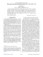
The various efficiency functions are combined to make two separate global efficiency
functions, one for long candidates and one for downstream candidates, which are used
as inputs to the fit to obtain the Cartesian observables z± . To smooth out statistical
fluctuations, an interpolation with a two-dimensional cubic spline function is performed to
give a continuous description of the efficiency ε(m2+ , m2− ), as shown in figure 1.


0.8
2
1.5

1
3

LHCb
Simulation

2.5
0.8
2

arbitrary units

2.5

m2+ (GeV2)

LHCb
Simulation

arbitrary units

m2+ (GeV2)

1
3

1.5
0.6

0.6

1

1

0.5

0.5
2

3

0.4

1

2

m2− (GeV )

2

3

0.4

2

m2− (GeV )

Figure 1. Variation of signal efficiency across the phase space for (left) long and (right) downstream
candidates.

mass, and taking the results of the invariant mass fit as inputs, as explained in section 5.2.
The cfit [45] library has been used to perform these fits. Candidate events are divided into
four subsamples, according to KS0 type (long or downstream), and whether the candidate
is identified as a B 0 or B 0 -meson decay. In the B-candidate invariant mass fit, the B 0
and B 0 samples are combined, since identical distributions are expected for this variable,
whilst in the CP violation observables fit (CP fit) they are kept separate.
5.1

Invariant mass fit of B 0 → DK ∗0 candidates

An unbinned extended maximum likelihood fit to the reconstructed invariant mass distributions of the B 0 candidates in the range [4900, 5800] MeV determines the signal and
background yields. The long and downstream subsamples are fitted simultaneously. The

total PDF includes several components: the B 0 → DK ∗0 signal PDF, background PDFs
(
)
0 → D ∗ K ∗0
for Bs0 → DK ∗0 decays, combinatorial background, partially reconstructed B(s)
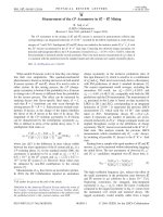
decays and misidentified B 0 → Dρ0 decays, as illustrated in figure 2.
The fit model is similar to that used in the analysis of B 0 → DK ∗0 decays with D-meson
decays to two-body final states [25]. The B 0 → DK ∗0 and Bs0 → DK ∗0 components are
each described as the sum of two Crystal Ball functions [46] sharing the same central value,
with the relative yields of the two functions and the tail parameters fixed from simulation.
The separation between the central values of the B 0 → DK ∗0 and Bs0 → DK ∗0 PDFs is
fixed to the known B 0 -Bs0 mass difference. The ratio of the B 0 → DK ∗0 and Bs0 → DK ∗0
yields is constrained to be the same in both the long and downstream subsamples. The
combinatorial background is described with an exponential PDF. Partially reconstructed
(
)
0 → D ∗ K ∗0 decays are described with non-parametric functions obtained by applying
B(s)
kernel density estimation [47] to distributions of simulated events. These distributions depend on the helicity state of the D∗0 meson. Due to parity conservation in D∗0 → D0 γ and
D∗0 → D0 π 0 decays, two of the three helicity amplitudes have the same invariant mass distribution. The Bs0 → D∗ K ∗0 PDF is therefore a linear combination of two non-parametric

–7–

JHEP08(2016)137

1


LHCb

B0→ DK*0
B0s→ DK*0

80

Combinatorial

60

B0→ D*K*0
B0s→ D*K*0

40

B0→ Dρ0

20
0

5000

5200

5400

5600

5800

m(DK*) (MeV)

Figure 2. Invariant mass distribution for B 0 → DK ∗0 long and downstream candidates. The fit
result, including signal and background components, is superimposed (solid blue). The points are
data, and the different fit components are given in the legend. The two vertical lines represent the
signal region in which the CP fit is performed.

functions, with the fraction of the longitudinal polarisation in the Bs0 → D∗ K ∗0 decays
unknown and accounted for with a free parameter in the fit. Each of the two functions describing the different helicity states is a weighted sum of non-parametric functions obtained
from simulated Bs0 → D∗ (D0 γ)K ∗0 and Bs0 → D∗ (D0 π 0 )K ∗0 decays, taking into account
the known D∗0 → D0 π 0 and D∗0 → D0 γ branching fractions [48] and the appropriate efficiencies. The PDF for B 0 → D∗ K ∗0 decays is obtained from that for Bs0 → D∗ K ∗0 decays,
by applying a shift corresponding to the known B 0 -Bs0 mass difference. In the nominal fit,
the polarisation fraction is assumed to be the same for B 0 → D∗ K ∗0 and Bs0 → D∗ K ∗0
decays. The effect of this assumption is taken into account in the systematic uncertainties.
The B 0 → Dρ0 component is also described with a non-parametric function obtained from
the simulation, using a data-driven calibration to describe the pion-kaon misidentification
efficiency. This component has a very low yield and, to improve the stability of the fit, a
Gaussian constraint is applied, requiring the ratio of yields of B 0 → Dρ0 and Bs0 → DK ∗0
to be consistent with its expected value.
The fitted distribution is shown in figure 2. The resulting signal and background yields
in a ±25 MeV range around the B 0 mass are given in table 1. This range corresponds to
the signal region over which the CP fit is performed.
5.2

CP fit

A simultaneous unbinned maximum likelihood fit to the four subsamples is performed to
determine the CP violation observables z± . The value of the coherence factor is fixed to the

–8–

JHEP08(2016)137

Candidates / [18 MeV]

100


Component

Yield
Downstream

Total

B 0 → DK ∗0

29 ± 5

60 ± 8

89 ± 11

Bs0 → DK ∗0

0.59 ± 0.12

1.21 ± 0.23

1.8 ± 0.3

9.6 ± 1.0

16.1 ± 1.4

25.7 ± 1.7

0.06 ± 0.02

0.06 ± 0.02

0.12 ± 0.03

4.1 ± 0.8

7.9 ± 1.3

11.9 ± 1.7

0.20 ± 0.05

0.37 ± 0.09

0.57 ± 0.11

14.5 ± 1.3

25.6 ± 1.8

40.1 ± 2.4

Combinatorial

D∗ K ∗0

B0 →

Bs0 → D∗ K ∗0
B0 →

Dρ0

Total background

Table 1. Signal and background yields in the signal region, ±25 MeV around the B 0 mass, obtained
from the invariant mass fit. Total yields, as well as separate yields for long and downstream
candidates, are given.

central value of κ = 0.958+0.005+0.002
−0.010−0.045 , as measured in the recent LHCb amplitude analysis
0
+
−
of B → DK π decays [30]. The negative logarithm of the likelihood,
− ln L = −

Nc fcmass (mB ; qc mass )fcB

ln
B 0 cand.

+

model

0

model

(m2+ , m2− ; z± , κ, qc model )

c

B 0 cand.

−

0

Nc fcmass (mB ; qc mass )fcB

ln

(m2+ , m2− ; z± , κ, qc model )

(5.1)

c

Nc ,
c

is minimised, where c indexes the different signal and background components, Nc is the

yield for each category, fcmass is the invariant mass PDF determined in the previous section,
qc mass are the mass PDF parameters, fcB model is the amplitude PDF and qc model are its
parameters other than z± and κ, which have been included explicitly.
The non-uniformity of the selection efficiency over the D → KS0 π + π − phase space is
accounted for by including the function ε(m2+ , m2− ), introduced in section 4, within the
fcB model PDF:
fcB

model

(m2+ , m2− ; z± , κ, qc model ) = Fc (m2+ , m2− ; z± , κ, qc model ) ε(m2+ , m2− ),

(5.2)

where Fc is the PDF of the amplitude model.
The model describing the amplitude of the D → KS0 π + π − decay over the phase
space, Af m2+ , m2− , is identical to that used previously by the BaBar [19, 49] and
LHCb [23] collaborations. An isobar model is used to describe P -wave (including ρ(770)0 ,
ω(782), Cabibbo-allowed and doubly Cabibbo-suppressed K ∗ (892)± and K ∗ (1680)− ) and
D-wave (including f2 (1270) and K2∗ (1430)± ) contributions. The Kπ S-wave contribution
(K0∗ (1430)± ) is described using a generalised LASS amplitude [50], whilst the ππ S-wave

–9–

JHEP08(2016)137

Long


x− = −0.15 ± 0.14,

y− =

0.25 ± 0.15,

x+ =

0.05 ± 0.24,

y+ = −0.65

+0.24
−0.23 ,

where the uncertainty is statistical only. The correlation matrix is
x − y− x + y +


1


0.14


 0

0

0.14
1
0

0

0

0




0 
,

1 0.14

0.14 1
0

and the corresponding likelihood contours for z± are shown in figure 5.
1

As previously noted in ref. [23], the model implemented by BaBar [49] differs from the formulation
described therein. One of the two Blatt-Weisskopf coefficients was set to unity, and the imaginary part
of the denominator of the Gounaris-Sakurai propagator used the mass of the resonant pair, instead of the
mass associated with the resonance. The model used herein replicates these features without modification.
It has been verified that changing the model to use an additional centrifugal barrier term and a modified
Gounaris-Sakurai propagator has a negligible effect on the measurements.

– 10 –

JHEP08(2016)137

contribution is treated using a P -vector approach within the K-matrix formalism. All
parameters of the model are fixed in the fit to the values determined in ref. [49].1
All components included in the fit of the B-meson mass spectrum are included in the
fit for the CP violation observables, with the exception of the B 0 → D∗ K ∗0 background,
because its yield within the signal region is negligible (table 1). CP violation is neglected
for Bs0 → DK ∗0 and Bs0 → D∗ K ∗0 decays, since their Cabbibo-suppressed contributions are
negligible. The relevant PDFs are therefore FB 0 →D(∗) K ∗0 = P(A¯f , 0, 0) and FB 0 →D(∗) K ∗0 =
s
s
P(Af , 0, 0), where P is defined in eq. (1.4). For background arising from misidentified
B 0 → Dρ0 events, the B flavour state cannot be determined, resulting in an incoherent
sum of D0 and D0 contributions: FB 0 →Dρ0 = (|Af |2 + |A¯f |2 )/2.
The combinatorial background is composed of two contributions: one from non-D candidates, and the other from real D mesons combined with random tracks. Combinatorial
D candidates arise from random combinations of four charged tracks, incorrectly reconstructed as a D → KS0 π + π − decay, and this contribution is assumed to be distributed
uniformly over phase space, FComb, non−D = 1, consistent with what is seen in the data.
Background from real D candidates arises when the K ∗ (892)0 candidate is reconstructed
from random tracks. Consequently, the B-meson flavour is unknown, resulting in an incoherent sum, FComb, real D = (|Af |2 + |A¯f |2 )/2. The relative proportions of non-D and real
D meson backgrounds (O(30%)) are fixed using the results of a fit to the reconstructed
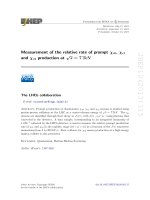
invariant mass of the D candidates in the signal B mass region. Figures 3 and 4 show the
Dalitz plot and its projections, with the fit result superimposed, for B 0 and B 0 candidates,
respectively. A blinding procedure was used to obscure the values of the CP parameters
until all aspects of the analysis were finalised. The measured values are


Candidates / [0.13 GeV2]

m2− (GeV2)

3

LHCb (a)

2.5
2
1.5
1
0.5
1

2

10
8
6
4
2
0

3

LHCb (b)

12

1

2

18

Candidates / [0.09 GeV2]

Candidates / [0.13 GeV2]

m2+ (GeV )

LHCb (c)

16
14
12
10
8
6
4
2
0

1

16

2

m2+ (GeV )

LHCb (d)

14

12
10
8
6
4
2
0

2

m2− (GeV2)

0.5

1

1.5

m20 (GeV2)

Figure 3. Selected B 0 → DK ∗0 candidates, shown as (a) the Dalitz plot, and its projections on
(b) m2− , (c) m2+ and (d) m20 . The line superimposed on the projections corresponds to the fit result
and the points are data.

6

Systematic uncertainties

Several sources of systematic uncertainty on the evaluation of z± are considered, and are
summarised in table 2. Unless otherwise stated, for each source considered, the CP fit is

repeated and the differences in the z± values compared to the nominal results are taken as
the systematic uncertainties.
The uncertainty on the description of the efficiency variation across the D-meson decay
phase space arises from several sources. Statistical uncertainties arise due to the limited
sizes of the simulated samples used to determine the nominal efficiency function and of
the calibration samples used to obtain the data-driven corrections to the PID and hardware trigger efficiencies. Large numbers of alternative efficiency functions are created by
smearing these quantities according to their uncertainties. For each fitted CP parameter,
the residual for a given alternative efficiency function is defined as the difference between
its value obtained using this function, and that obtained in the nominal fit. The width of
the obtained distribution of residuals is taken as the corresponding systematic uncertainty.
Additionally, since the nominal fit is performed using an efficiency function obtained from
the simulation applying only BDTA, the fit is repeated using an alternative efficiency function obtained using BDTB, and an uncertainty extracted. The fit is also performed with

– 11 –

JHEP08(2016)137

2


Candidates / [0.13 GeV2]

m2− (GeV2)

3

LHCb (a)

2.5
2

1.5
1

14
12
10
8
6
4

2

2

(GeV )

LHCb (c)

10
8
6
4
2
1

1

2

Candidates / [0.09 GeV2]

12

0

3

m2+

12

LHCb (d)

10
8
6
4
2
0

2

m2− (GeV2)

0.5

1

1.5

m20 (GeV2)

2

m2+ (GeV )

y±

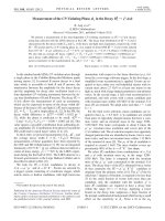
Figure 4. Selected B 0 → DK ∗0 candidates, shown as (a) the Dalitz plot, and its projections on
(b) m2− , (c) m2+ and (d) m20 . The line superimposed on the projections corresponds to the fit result
and the points are data.

1

LHCb

0

B

0

-1
B0

-1

0

1

x±
Figure 5. Likelihood contours at 68.3% and 95.5% confidence level for (x+ , y+ ) (red) and (x− , y− )
(blue), obtained from the CP fit.

– 12 –

JHEP08(2016)137

1

Candidates / [0.13 GeV2]

LHCb (b)

16

2

0.5

0

18


Source of uncertainty

δx−

δy−

δx+

δy+

Efficiency

5.4

1.1

11

1.8

Invariant mass fit

12

21

15

48

Migration over the phase space

5.3

1.8

6.2

3.0

Misreconstructed signal

7.7

6.6

10

7.1

Non-D background

20

15

28

47

Real D background

0.1

0.4

0.2

1.0

CP violation in Bs0 → D∗ K ∗0

1.5

0.8

4.0

1.6

0.6

1.4

0.8

2.3

0.1

0.7

0.5

1.6

4.8

2.4

8.5

2.6

CP fit bias

5

49

11

40

Total experimental

26 (19%)

56 (37%)

39 (16%)

78 (33%)

8 (5%)

7 (5%)

10 (4%)

5 (2%)

Background description

D0 π+ π+ π−

contribution

Λ0b → D0 pπ − contribution
K∗

coherence factor (κ)

Total model-related (see table 3)

Table 2. Summary of the systematic uncertainties on z± , in units of (10−3 ). The total experimental
and total model-related uncertainties are also given as percentages of the statistical uncertainties.

alternative efficiency functions obtained by varying the fraction of candidates triggered by
at least one product of the signal decay chain. Finally, for a few variables used in the BDT,
a small difference is observed between the simulation and the background-subtracted data
sample. To account for this difference, the simulated events are reweighted to match the
data, and the fit is repeated with the resulting efficiency function.
The B-meson invariant mass fit result is used to fix the fractions of signal and background and the parameters of the B 0 mass PDF shapes in the CP fit. A large number

of pseudoexperiments is generated, in which the free parameters of the invariant mass fit
are varied within their uncertainties, taking into account their correlations. The CP fit
is repeated for each variation. For each CP parameter, the width from a Gaussian fit to
the resulting residual distribution is taken as the associated systematic uncertainty. This
is the dominant contribution to the invariant mass fit systematic uncertainty quoted in
table 2. Other uncertainties due to assumptions in the invariant mass fit are evaluated by
allowing the B 0 → DK ∗0 /Bs0 → DK ∗0 yield ratio to be different for long and downstream
categories, by varying the B 0 → Dρ0 /Bs0 → DK ∗0 yield ratio, by varying the Crystal Ball
PDF parameters within their uncertainties and by testing alternatives to the Crystal Ball
(
)
0 → D ∗ K ∗0 background
PDFs. The proportions of D∗0 → D0 γ and D∗0 → D0 π 0 in the B(s)
description are also varied, and the effect of neglecting the B 0 → D∗ K ∗0 component in the
CP fit is evaluated.
The systematic uncertainty due to the finite resolution in m2± is evaluated with a large
number of pseudoexperiments. One nominal pseudodata sample is generated, with z± fixed

– 13 –

JHEP08(2016)137

B+ →


– 14 –

JHEP08(2016)137

to the values obtained from data. A large number of alternative samples are generated from

the nominal one by smearing the m2± coordinates of each event according to the resolution
found in simulation and taking correlations into account. For each CP parameter, the
width of the residual distribution is taken as the systematic uncertainty.
The misreconstruction of B 0 → DK ∗0 signal events is also studied. This can occur e.g.
when the wrong final state pions of a real signal event are combined in the reconstruction
of the D-meson candidate, leading to migration of this event within the D-decay phase
space. The uncertainty corresponding to this effect is evaluated using pseudoexperiments.
The effect of signal misreconstruction due to K ∗0 –K ∗0 misidentification, corresponding
to a (K ± π ∓ ) → (π ± K ∓ ) misidentification, is found to be negligible thanks to the PID
requirements placed on the K ∗0 daughters.
The uncertainty arising from the background description is evaluated for several
sources. The CP fit is repeated with the fractions of the two categories of combinatorial
background (non-D and real D candidates) varied within their uncertainties from the fit
to the D invariant mass distribution. Additionally, since in the nominal fit the non-D candidates are assumed to be uniformly distributed over the phase space of the D → KS0 π + π −
decay, the fit is repeated changing this contribution to the sum of a uniform distribution
and a K ∗ (892)± resonance. The relative proportions of the two components are fixed based
on the m2± distributions found in data. The fit is also repeated with the D-meson decay
model for the non-D component set to the distribution of data in the D mass sidebands.
The uncertainty arising from the poorly-known fraction of non-D and real D background
is the dominant systematic uncertainty for the x± parameters.
The description of the real D combinatorial background assumes that the probabilities
of a D0 or a D0 being present in an event are equal. The CP violation observables fit is
repeated with the decay model for this background changed to include a D0 –D0 production
asymmetry, whose value is set to the measured D± asymmetry (−1.0 ± 0.3) × 10−2 [51].
CP violation is neglected in the Bs0 → D∗ K ∗0 decay nominal description. The CP
fit is repeated with the inclusion of a small component describing the suppressed decay
amplitude of Bs0 → D∗0 K ∗0 , with CP violation parameters for this component fixed to
γ = 73.2◦ , rBs0 = 0.02 and δBs0 = {0◦ , 45◦ , 90◦ , 135◦ , 180◦ , 225◦ , 270◦ , 315◦ }. The model
used to describe Bs0 → D∗ K ∗0 decays consists of an incoherent sum of D∗0 → D0 π 0 and
D∗0 → D0 γ contributions. Between the D∗0 → D0 π 0 and D∗0 → D0 γ decays, there is an

effective strong phase shift of π that is taken into account [52].
The systematic uncertainties arising from the inclusion of background from misreconstructed B + → D0 π + π + π − and Λ0b → D0 pπ − decays are evaluated, by adding these
components into the fit model. The CP fit is also repeated with the K ∗ (892)0 coherence
factor κ varied within its uncertainty [30].
The CP fit is verified using one thousand data-sized pseudoexperiments. In each
experiment, the signal and background yields, as well as the distributions used in the
generation, are fixed to those found in data. The fitted values of z± show biases smaller
than the statistical uncertainties, and are included as systematic uncertainties. These biases
are due to the current limited statistics and are found to reduce in pseudoexperiments
generated with a larger sample size.


− ππ S-wave: the F -vector model is changed to use two other solutions of the K-matrix
(from a total of three) determined from fits to scattering data [53] (a), (b). The slowly
varying part of the nonresonant term of the P -vector is removed (c).
− Kπ S-wave: the generalised LASS parametrisation used to describe the K0∗ (1430)±
resonance, is replaced by a relativistic Breit-Wigner propagator with parameters
taken from ref. [54] (d).
− ππ P-wave: the Gounaris-Sakurai propagator is replaced by a relativistic BreitWigner propagator [19, 49] (e).
− Kπ P-wave: the mass and width of the K ∗ (1680)− resonance are varied by their
uncertainties from ref. [50] (f)−(i).
− ππ D-wave: the mass and width of the f2 (1270) resonance are varied by their uncertainties from ref. [24] (j)−(m).
− Kπ D-wave: the mass and width of the K2∗ (1430)± resonance are varied by their
uncertainties from ref. [55] (n)−(q).
− The radius of the Blatt-Weisskopf centrifugal barrier factors, rBW , is changed from
1.5 GeV−1 to 0.0 GeV−1 (r) and 3.0 GeV−1 (s).
− Two further resonances, K ∗ (1410)0 and ρ(1450), parametrised with relativistic BreitWigner propagators, are included in the model [19, 49] (t).
− The Zemach formalism used for the angular distribution of the decay products is
replaced by the helicity formalism [19, 49] (u).
It results in total systematic uncertainties arising from the choice of amplitude model of

δx− = 8 × 10−3 ,
δy− = 7 × 10−3 ,
δx+ = 10 × 10−3 ,
δy+ = 5 × 10−3 .
The different systematic uncertainties are combined, assuming that they are independent to obtain the total experimental uncertainties. Depending on the (x± , y± ) parameters,
the leading systematic uncertainties arise from the invariant mass fit, the description of the
non-D background and the fit biases. A larger data sample is expected to reduce all three of

– 15 –

JHEP08(2016)137

To evaluate the systematic uncertainty due to the choice of amplitude model for
D → KS0 π + π − , one million B 0 → DK ∗0 and one million Bs0 → DK ∗0 decays are simulated
according to the nominal decay model, with the Cartesian observables fixed to the nominal
fit result. These simulated decays are fitted with alternative models, each of which includes
a single modification with respect to the nominal model, as described in the next paragraph.
Each of these alternative models is first used to fit the simulated Bs0 → DK ∗0 decays to determine values for the resonance coefficients of the model. Those coefficients are then fixed
in a second fit, to the simulated B 0 → DK ∗0 decays, to obtain z± . The systematic uncertainties are taken to be the signed differences in the values of z± from the nominal results.
The following changes, labelled (a)-(u), are applied in the alternative models, leading
to the uncertainties shown in table 3:


Description

δx−

δy−

δx+

δy+

(a)

K-matrix 1st solution

−2

0.9

2

1

(b)

K-matrix 2nd solution

0.3

0.3

0.0

−0.5

(c)

Remove slowly varying

−0.7

0.2

0.5

0.6

2

3

−1

3

0.7

0.0

−0.1

0.8

m + δm

−0.0

0.6

0.1

0.5

m − δm

−0.2

−0.5

0.2

−0.9

Γ + δΓ

−0.2

0.2

0.0

−0.2

(i)

Γ − δΓ

0.2

−0.1

0.5

−0.2

(j)

m + δm

−0.1

0.0

0.3

−0.2

m − δm

−0.0

0.1

0.2

−0.2

Γ + δΓ

−0.0

0.0

0.2

−0.2

(m)

Γ − δΓ

−0.1

0.0

0.2

−0.2

(n)

m + δm

0.3

0.2

0.2

−0.2

m − δm

−0.4

−0.2

0.3

−0.1

Γ + δΓ

−0.2

0.2

0.1

−0.2

Γ − δΓ

part in P -vector
(d)

→ relativistic Breit-Wigner
Gounaris-Sakurai

→ relativistic Breit-Wigner

(f)
(g)
(h)

(k)
(l)

(o)
(p)

K ∗ (1680)

f2 (1270)

K2∗ (1430)

0.1

−0.1

0.3

−0.2

(r)

rBW =

0.0 GeV−1

−2

0.7

−1

−0.3

(s)

rBW = 3.0 GeV−1

4

−2

4

2

and ρ(1450) −0.2

−0.2

0.3

−0.3

−6

6

−8

2

8

7

10

5

(q)

K ∗ (1410)

(t)

Add

(u)

Helicity formalism
Total model related

Table 3. Model related systematic uncertainties for each alternative model, in units of (10 −3 ).

The relative signs indicate full correlation or anti-correlation.

these uncertainties. Whilst not intrinsically statistical in nature, the systematic uncertainty
due to the description of the non-D background is presently evaluated using a conservative approach due to lack of statistics. The total systematic uncertainties, including the
model-related uncertainties, are significantly smaller than the statistical uncertainties.

– 16 –

JHEP08(2016)137

(e)

Generalised LASS


7

Determination of the parameters γ, rB 0 and δB 0

To determine the physics parameters rB 0 , δB 0 and γ from the fitted Cartesian observables
z± , the relations
x± = rB 0 cos(δB 0 ± γ),
(7.1)
y± = rB 0 sin(δB 0 ± γ),

L(x− , y− , x+ , y+ |rB 0 , δB 0 , γ).

(7.2)

All statistical and systematic uncertainties on z± are accounted for, as well as the statistical

correlation between z± . Since the precision of the measurement is statistics dominated, correlations between the systematic uncertainties are ignored. Central values for (rB 0 , δB 0 , γ)
are obtained by performing a scan of these parameters, to find the values that maximise
obs obs obs
obs are the measured values of the Cartesian
L(xobs
− , y− , x+ , y+ |rB 0 , δB 0 , γ), where z±
observables. Associated confidence intervals may be obtained either from a simple profilelikelihood method, or using the Feldman-Cousins approach [57] combined with a “plugin”
method [58]. Confidence level curves for (rB 0 , δB 0 , γ) obtained using the latter method are
shown in figures 6, 7 and 8. The measured values of z± are found to correspond to
◦

γ = 80+21
−22 ,
rB 0 = 0.39 ± 0.13,
◦

δB 0 = 197+24
−20 .
Intrinsic to the method used in this analysis [12], there is a two-fold ambiguity in the solution; the Standard Model solution (0 < γ < 180)◦ is chosen. Two-dimensional confidence
level curves obtained using the profile-likelihood method are shown in figures 9 and 10.

8

Conclusion

An amplitude analysis of B 0 → DK ∗0 decays, employing a model description of the D →
KS0 π + π − decay, has been performed using data corresponding to an integrated luminosity
of 3 fb−1 , recorded by LHCb at a centre-of-mass energy of 7 TeV in 2011 and 8 TeV in
2012. The measured values of the CP violation observables x± = rB 0 cos (δB 0 ± γ) and
y± = rB 0 sin (δB 0 ± γ) are

x− = −0.15 ± 0.14 ± 0.03 ± 0.01,
y− =

0.25 ± 0.15 ± 0.06 ± 0.01,

x+ =

0.05 ± 0.24 ± 0.04 ± 0.01,

y+ = −0.65

+0.24
−0.23

– 17 –

± 0.08 ± 0.01,

JHEP08(2016)137

must be inverted. This is done using the GammaCombo package, originally developed for the
frequentist combination of γ measurements by the LHCb collaboration [7, 56]. A global
likelihood function is built, which gives the probability of observing a set of z± values given
the true values (rB 0 , δB 0 , γ),


1−CL

1

LHCb
0.8
80+21
−22

0.6
0.4

68.3%

95.5%
0

50

100

150

γ [°]

1−CL

Figure 6. Confidence level curve on γ, obtained using the “plugin” method [58].

1

LHCb

0.8

0.39+0.13
−0.13

0.6
0.4

68.3%

0.2
95.5%
0

0.2

0.4

0.6

0.8

rB0
Figure 7. Confidence level curve on rB 0 , obtained using the “plugin” method [58].

where the first uncertainties are statistical, the second are systematic and the third are
due to the choice of amplitude model used to describe the D → KS0 π + π − decay. These
are the most precise measurements of these observables related to the neutral channel
B 0 → DK ∗0 . They place constraints on the magnitude of the ratio of the interfering Bmeson decay amplitudes, the strong phase difference between them and the CKM angle γ,

– 18 –

JHEP08(2016)137

0.2


1−CL

1

LHCb

0.8
197+24
−20

0.6
68.3%

0.2
95.5%
0

100

200

300

δB0 [°]

rB0

Figure 8. Confidence level curve on δB 0 , obtained using the “plugin” method [58]. Only the
δB 0 solution corresponding to 0 < γ < 180◦ is highlighted; the other maximum is due to the
(δB 0 , γ) → (δB 0 + π, γ + π) ambiguity.

1

LHCb

0.8
0.6
0.4
0.2
contours hold 68%, 95% CL

0
0

50

100

150

γ [°]
Figure 9. Two-dimensional confidence level curves in the (γ, rB 0 ) plane, obtained using the profilelikelihood method.

– 19 –

JHEP08(2016)137

0.4


δB0 [°]

350

LHCb
300
250
200

contours hold 68%, 95% CL

0

50

100

150

γ [°]
Figure 10. Two-dimensional confidence level curves in the (γ, δB 0 ) plane, obtained using the
profile-likelihood method.

giving the values
◦

γ = 80+21
−22 ,
rB 0 = 0.39 ± 0.13,
◦

δB 0 = 197+24
−20 .
Here, rB 0 and δB 0 are defined for a Kπ mass region of ±50 MeV around the K ∗ (892)0
mass and for an absolute value of the cosine of the K ∗0 decay angle greater than 0.4.
These results are consistent with, and have lower total uncertainties than those reported
in ref. [28], where a model independent analysis method is used. The two results are based
on the same data set and cannot be combined. The consistency shows that at the current
level of statistical precision the assumptions used to obtain the present result are justified.

Acknowledgments
We express our gratitude to our colleagues in the CERN accelerator departments for
the excellent performance of the LHC. We thank the technical and administrative staff
at the LHCb institutes. We acknowledge support from CERN and from the national
agencies: CAPES, CNPq, FAPERJ and FINEP (Brazil); NSFC (China); CNRS/IN2P3
(France); BMBF, DFG and MPG (Germany); INFN (Italy); FOM and NWO (The Netherlands); MNiSW and NCN (Poland); MEN/IFA (Romania); MinES and FANO (Russia);
MinECo (Spain); SNSF and SER (Switzerland); NASU (Ukraine); STFC (United Kingdom); NSF (U.S.A.). We acknowledge the computing resources that are provided by CERN,
IN2P3 (France), KIT and DESY (Germany), INFN (Italy), SURF (The Netherlands), PIC

– 20 –

JHEP08(2016)137

150

(Spain), GridPP (United Kingdom), RRCKI and Yandex LLC (Russia), CSCS (Switzerland), IFIN-HH (Romania), CBPF (Brazil), PL-GRID (Poland) and OSC (U.S.A.). We are
indebted to the communities behind the multiple open source software packages on which we
depend. Individual groups or members have received support from AvH Foundation (Germany), EPLANET, Marie Sklodowska-Curie Actions and ERC (European Union), Conseil
G´en´eral de Haute-Savoie, Labex ENIGMASS and OCEVU, R´egion Auvergne (France),
RFBR and Yandex LLC (Russia), GVA, XuntaGal and GENCAT (Spain), Herchel Smith
Fund, The Royal Society, Royal Commission for the Exhibition of 1851 and the Leverhulme
Trust (United Kingdom).

References
[1] N. Cabibbo, Unitary symmetry and leptonic decays, Phys. Rev. Lett. 10 (1963) 531 [INSPIRE].
[2] M. Kobayashi and T. Maskawa, CP violation in the renormalizable theory of weak
interaction, Prog. Theor. Phys. 49 (1973) 652 [INSPIRE].
[3] J. Brod and J. Zupan, The ultimate theoretical error on γ from B → DK decays, JHEP 01
(2014) 051 [arXiv:1308.5663] [INSPIRE].
[4] BaBar collaboration, J.P. Lees et al., Observation of direct CP-violation in the
measurement of the Cabibbo-Kobayashi-Maskawa angle γ with B ± → D(∗) K (∗)± decays,
Phys. Rev. D 87 (2013) 052015 [arXiv:1301.1029] [INSPIRE].
[5] Belle collaboration, K. Trabelsi, Study of direct CP in charmed B decays and measurement
of the CKM angle γ at Belle, arXiv:1301.2033 [INSPIRE].
[6] Belle and BaBar collaborations, A.J. Bevan et al., The physics of the B factories, Eur.
Phys. J. C 74 (2014) 3026 [arXiv:1406.6311] [INSPIRE].
[7] LHCb collaboration, Improved constraints on γ: CKM2014 update, LHCb-CONF-2014-004,
CERN, Geneva Switzerland (2014).
[8] CKMfitter Group collaboration, J. Charles et al., CP violation and the CKM matrix:
assessing the impact of the asymmetric B factories, Eur. Phys. J. C 41 (2005) 1
[hep-ph/0406184] [INSPIRE].
[9] J. Charles et al., Current status of the Standard Model CKM fit and constraints on ∆F = 2
new physics, Phys. Rev. D 91 (2015) 073007 [arXiv:1501.05013] [INSPIRE].
[10] UTfit collaboration, M. Bona et al., The 2004 UTfit collaboration report on the status of the

unitarity triangle in the standard model, JHEP 07 (2005) 028 [hep-ph/0501199] [INSPIRE].
[11] A. Bondar, Proceedings of BINP special analysis meeting on Dalitz, unpublished, (2002).
[12] A. Giri, Y. Grossman, A. Soffer and J. Zupan, Determining γ using B ± → DK ± with
multibody D decays, Phys. Rev. D 68 (2003) 054018 [hep-ph/0303187] [INSPIRE].
[13] Belle collaboration, H. Aihara et al., First measurement of φ3 with a model-independent
Dalitz plot analysis of B ± → DK ± , D → Ks π + π − decay, Phys. Rev. D 85 (2012) 112014
[arXiv:1204.6561] [INSPIRE].

– 21 –

JHEP08(2016)137

Open Access. This article is distributed under the terms of the Creative Commons
Attribution License (CC-BY 4.0), which permits any use, distribution and reproduction in
any medium, provided the original author(s) and source are credited.


[14] LHCb collaboration, Measurement of the CKM angle γ using B ± → DK ± with
D → KS0 π + π − , KS0 K + K − decays, JHEP 10 (2014) 097 [arXiv:1408.2748] [INSPIRE].
[15] LHCb collaboration, A model-independent Dalitz plot analysis of B ± → DK ± with
D → KS0 h+ h− (h = π, K) decays and constraints on the CKM angle γ, Phys. Lett. B 718
(2012) 43 [arXiv:1209.5869] [INSPIRE].
[16] CLEO collaboration, J. Libby et al., Model-independent determination of the strong-phase
¯ 0 → K 0 h+ h− (h = π, K) and its impact on the measurement
difference between D0 and D
S,L
of the CKM angle γ/φ3 , Phys. Rev. D 82 (2010) 112006 [arXiv:1010.2817] [INSPIRE].

[18] BaBar collaboration, B. Aubert et al., Improved measurement of the CKM angle γ in
B ∓ → D(∗) K (∗∓) decays with a Dalitz plot analysis of D decays to KS0 π + π − and KS0 K + K − ,

Phys. Rev. D 78 (2008) 034023 [arXiv:0804.2089] [INSPIRE].
[19] BaBar collaboration, P. del Amo Sanchez et al., Evidence for direct CP-violation in the
measurement of the Cabibbo-Kobayashi-Maskawa angle γ with B ∓ → D(∗) K (∗)∓ decays,
Phys. Rev. Lett. 105 (2010) 121801 [arXiv:1005.1096] [INSPIRE].
[20] Belle collaboration, A. Poluektov et al., Measurement of φ3 with Dalitz plot analysis of
B ± → D(∗) K ± decay, Phys. Rev. D 70 (2004) 072003 [hep-ex/0406067] [INSPIRE].
[21] Belle collaboration, A. Poluektov et al., Measurement of φ3 with Dalitz plot analysis of
B + → D(∗) K (∗)+ decay, Phys. Rev. D 73 (2006) 112009 [hep-ex/0604054] [INSPIRE].
[22] Belle collaboration, A. Poluektov et al., Evidence for direct CP-violation in the decay
B ± → D(∗) K ± , D → Ks π + π − and measurement of the CKM phase φ3 , Phys. Rev. D 81
(2010) 112002 [arXiv:1003.3360] [INSPIRE].
[23] LHCb collaboration, Measurement of CP violation and constraints on the CKM angle γ in
B ± → DK ± with D → KS0 π + π − decays, Nucl. Phys. B 888 (2014) 169 [arXiv:1407.6211]
[INSPIRE].
[24] Particle Data Group collaboration, K.A. Olive et al., Review of particle physics, Chin.
Phys. C 38 (2014) 090001 [INSPIRE].
[25] LHCb collaboration, Measurement of CP-violation parameters in B 0 → DK ∗0 decays, Phys.
Rev. D 90 (2014) 112002 [arXiv:1407.8136] [INSPIRE].
0

[26] BaBar collaboration, B. Aubert et al., Constraints on the CKM angle γ in B 0 → D K ∗0
0
and B 0 → D0 K ∗0 from a Dalitz analysis of D0 and D decays to KS π + π − , Phys. Rev. D 79
(2009) 072003 [arXiv:0805.2001] [INSPIRE].
[27] Belle collaboration, K. Negishi et al., First model-independent Dalitz analysis of
B 0 → DK ∗0 , D → KS0 π + π − decay, Prog. Theor. Exp. Phys. 2016 (2016) 043C01
[arXiv:1509.01098] [INSPIRE].
[28] LHCb collaboration, Model-independent measurement of the CKM angle γ using
B 0 → DK ∗0 decays with D → KS0 π + π − and KS0 K + K − , JHEP 06 (2016) 131
[arXiv:1604.01525] [INSPIRE].

[29] M. Gronau, Improving bounds on γ in B ± → DK ± and B ±,0 → DXs±,0 , Phys. Lett. B 557
(2003) 198 [hep-ph/0211282] [INSPIRE].

– 22 –

JHEP08(2016)137

[17] BaBar collaboration, B. Aubert et al., Measurement of γ in B ∓ → D(∗) K ∓ decays with a
Dalitz analysis of D → KS0 π − π + , Phys. Rev. Lett. 95 (2005) 121802 [hep-ex/0504039]
[INSPIRE].


[30] LHCb collaboration, Constraints on the unitarity triangle angle γ from Dalitz plot analysis
of B 0 → DK + π − decays, Phys. Rev. D 93 (2016) 112018 [arXiv:1602.03455] [INSPIRE].
[31] LHCb collaboration, The LHCb detector at the LHC, 2008 JINST 3 S08005 [INSPIRE].
[32] LHCb collaboration, LHCb detector performance, Int. J. Mod. Phys. A 30 (2015) 1530022
[arXiv:1412.6352] [INSPIRE].
[33] V.V. Gligorov and M. Williams, Efficient, reliable and fast high-level triggering using a
bonsai boosted decision tree, 2013 JINST 8 P02013 [arXiv:1210.6861] [INSPIRE].

[35] T. Sj¨
ostrand, S. Mrenna and P.Z. Skands, PYTHIA 6.4 physics and manual, JHEP 05
(2006) 026 [hep-ph/0603175] [INSPIRE].
[36] LHCb collaboration, Handling of the generation of primary events in Gauss, the LHCb
simulation framework, J. Phys. Conf. Ser. 331 (2011) 032047 [INSPIRE].
[37] D.J. Lange, The EvtGen particle decay simulation package, Nucl. Instrum. Meth. A 462
(2001) 152 [INSPIRE].
[38] P. Golonka and Z. Was, PHOTOS Monte Carlo: a precision tool for QED corrections in Z
and W decays, Eur. Phys. J. C 45 (2006) 97 [hep-ph/0506026] [INSPIRE].
[39] GEANT4 collaboration, J. Allison et al., GEANT4 developments and applications, IEEE

Trans. Nucl. Sci. 53 (2006) 270 [INSPIRE].
[40] GEANT4 collaboration, S. Agostinelli et al., GEANT4: a simulation toolkit, Nucl. Instrum.
Meth. A 506 (2003) 250 [INSPIRE].
[41] M. Clemencic et al., The LHCb simulation application, Gauss: design, evolution and
experience, J. Phys. Conf. Ser. 331 (2011) 032023 [INSPIRE].
[42] W.D. Hulsbergen, Decay chain fitting with a Kalman filter, Nucl. Instrum. Meth. A 552
(2005) 566 [physics/0503191] [INSPIRE].
[43] L. Breiman, J.H. Friedman, R.A. Olshen and C.J. Stone, Classification and regression trees,
Wadsworth international group, Belmont CA U.S.A. (1984).
[44] B.P. Roe, H.-J. Yang, J. Zhu, Y. Liu, I. Stancu and G. McGregor, Boosted decision trees, an
alternative to artificial neural networks, Nucl. Instrum. Meth. A 543 (2005) 577
[physics/0408124] [INSPIRE].
[45] J. Garra Tico, The cfit fitting package webpage, />[46] T. Skwarnicki, A study of the radiative cascade transitions between the Υ and Υ resonances,
Ph.D. thesis, DESY-F31-86-02, Institute of Nuclear Physics, Krakow Poland (1986)
[INSPIRE].
[47] K.S. Cranmer, Kernel estimation in high-energy physics, Comput. Phys. Commun. 136
(2001) 198 [hep-ex/0011057] [INSPIRE].
[48] BESIII collaboration, M. Ablikim et al., Precision measurement of the D∗0 decay branching
fractions, Phys. Rev. D 91 (2015) 031101 [arXiv:1412.4566] [INSPIRE].
¯ 0 mixing parameters
[49] BaBar collaboration, P. del Amo Sanchez et al., Measurement of D0 -D
using D0 → KS0 π + π − and D0 → KS0 K + K − decays, Phys. Rev. Lett. 105 (2010) 081803
[arXiv:1004.5053] [INSPIRE].

– 23 –

JHEP08(2016)137

[34] T. Sj¨
ostrand, S. Mrenna and P.Z. Skands, A brief introduction to PYTHIA 8.1, Comput.

Phys. Commun. 178 (2008) 852 [arXiv:0710.3820] [INSPIRE].


[50] D. Aston et al., A study of K − π + scattering in the reaction K − p → K − π + n at 11 GeV/c,
Nucl. Phys. B 296 (1988) 493 [INSPIRE].
[51] LHCb collaboration, Measurement of the D± production asymmetry in 7 TeV pp collisions,
Phys. Lett. B 718 (2013) 902 [arXiv:1210.4112] [INSPIRE].
[52] A. Bondar and T. Gershon, On φ3 measurements using B − → D∗ K − decays, Phys. Rev. D
70 (2004) 091503 [hep-ph/0409281] [INSPIRE].
[53] V.V. Anisovich and A.V. Sarantsev, K matrix analysis of the (IJ (P C) = 00++ )-wave in the
mass region below 1900 MeV, Eur. Phys. J. A 16 (2003) 229 [hep-ph/0204328] [INSPIRE].

[55] Particle Data Group collaboration, J. Beringer et al., Review of particle physics (RPP),
Phys. Rev. D 86 (2012) 010001 [INSPIRE].
[56] LHCb collaboration, Measurement of the CKM angle γ from a combination of B ± → Dh±
analyses, Phys. Lett. B 726 (2013) 151 [arXiv:1305.2050] [INSPIRE].
[57] G.J. Feldman and R.D. Cousins, A unified approach to the classical statistical analysis of
small signals, Phys. Rev. D 57 (1998) 3873 [physics/9711021] [INSPIRE].
[58] S. Bodhisattva, M. Walker and M. Woodroofe, On the unified method with nuisance
parameters, Statist. Sinica 19 (2009) 301 [INSPIRE].

– 24 –

JHEP08(2016)137

[54] E791 collaboration, E.M. Aitala et al., Dalitz plot analysis of the decay D+ → K − π + π + and
indication of a low-mass scalar Kπ resonance, Phys. Rev. Lett. 89 (2002) 121801
[hep-ex/0204018] [INSPIRE].