DSpace at VNU: High energy scattering of Dirac particles on smooth potentials
Bạn đang xem bản rút gọn của tài liệu. Xem và tải ngay bản đầy đủ của tài liệu tại đây (242.82 KB, 18 trang )
International Journal of Modern Physics A
Vol. 31, No. 23 (2016) 1650126 (18 pages)
c World Scientific Publishing Company
DOI: 10.1142/S0217751X16501268
High energy scattering of Dirac particles on smooth potentials
Int. J. Mod. Phys. A 2016.31. Downloaded from www.worldscientific.com
by NEW YORK UNIVERSITY on 08/28/16. For personal use only.
Nguyen Suan Han,∗,‡ Le Anh Dung,∗ Nguyen Nhu Xuan†,§ and Vu Toan Thang∗
∗ Department of Theoretical Physics,
Hanoi University of Science, Hanoi, Vietnam
† Department of Physics, Le Qui Don University, Hanoi, Vietnam
‡
§
Received 26 March 2016
Revised 9 June 2016
Accepted 15 July 2016
Published 19 August 2016
The derivation of the Glauber type representation for the high energy scattering amplitude of particles of spin 1/2 is given within the framework of the Dirac equation in the
Foldy–Wouthuysen (FW) representation and two-component formalism. The differential
cross-sections on the Yukawa and Gaussian potentials are also considered and discussed.
Keywords: Foldy–Wouthuysen representation; eikonal scattering theory.
PACS numbers: 11.80.−m, 04.60.−m
1. Introduction
Eikonal representation, or Glauber type representation, for the scattering amplitude of high energy particles with small scattering angles was first obtained in
Quantum Mechanics1 and, then, in Quantum Field Theory based on the Logunov–
Tavkhelidze quasipotential equation.2,3 The assumption of the smoothness of local
pseudo-potential4–6 allows us to explain successfully physical characteristics of high
energy scattering of hadrons. More generally, it leads to a simple qualitative model
of interactions between particles in the asymptotic region of high energy.
Eikonal representation for high energy scattering amplitude has been studied
by other authors.7–20 However, these investigations do not take into account the
spin structure of the scattered particles. Some authors included spin effects in their
studies,19,20 but their methods were not complete, or could not be applied for
various potentials. On the other hand, experiments showed that spin effects, for
example, the non-negligibility of the ratio of spin-flip to spin-nonflip amplitudes
and Coulomb-hadron interference,21–23 play an important role in many physical
processes, such as in the recent RHIC and LHC experiments.24,25 Moreover, present
1650126-1
Int. J. Mod. Phys. A 2016.31. Downloaded from www.worldscientific.com
by NEW YORK UNIVERSITY on 08/28/16. For personal use only.
N. S. Han et al.
investigations did not utilize the Foldy–Wouthuysen (FW) transformation which is
very convenient for passing to the quasiclassical approximation. Consequently, this
paper aims to generalize the eikonal representation for the scattering amplitude of
spinor particles, in particular, to establish the Glauber type representation for the
scattering amplitude of spin 1/2 particles on smooth potentials at high energies
within the framework of the Dirac equation in an external field after using the FW
transformation.26–32
The paper is organized as follows. In Sec. 2, we obtain the Dirac equation
in an external field in the FW representation. This representation has a special
place in the field of relativistic quantum mechanics due to the following properties.
First, Hamiltonian and quantum mechanical operators for relativistic particles in
external fields in the FW representation are similar to those in the nonrelativistic
quantum mechanics. Second, the quasiclassical approximation and the classical limit
of relativistic quantum mechanics can be obtained by a replacement of operators in
quantum-mechanical Hamiltonian and equations of motion with the corresponding
classical quantities.28–31 This property is significant since most quantum effects are
measured using classical apparatuses. Moreover, the FW representation is perfect
for a description of spin effects which will be discussed later. We need also to
mention that the relativistic FW transformation is widely and successfully used
in quantum chemistry (see Refs. 35–41). In Sec. 3, employing the smoothness of
external potentials and the Dirac equation in the FW representation, we end up
with the Glauber type representation for the high energy scattering amplitude of
spin −1/2 particles. In Sec. 4, the analytical expressions of the differential crosssection in the Yukawa and Gaussian potentials are derived. The contribution of
terms in the FW Hamiltonian to the scattering processes discussed. The results
and possible generalizations of this approach are also discussed.
2. Foldy Wouthuysen Transformation for the Dirac Equation in
External Field
In general, there are two regular ways to perform the FW representation of the
Dirac Hamiltonian: one approach gives a series of relativistic corrections to the
nonrelativistic Schr¨odinger Hamiltonian;26,27,32 the other approach allows one to
obtain a compact expression for the relativistic FW Hamiltonian (see Refs. 28–31,
33, 34 and references therein). In this section, we utilize the method in Ref. 34.
The Dirac equation for a particle with charge e = q in an external electromagnetic field Vµ (V, A ) is given by
∂Ψ(r, t)
= HD Ψ(r , t)
dt
with the Dirac Hamiltonian HD and bi-spinor Ψ defined as follows:
i
(2.1)
HD = βm + O + E ,
(2.2)
ψ
,
η
(2.3)
Ψ=
1650126-2
High energy scattering of Dirac particles on smooth potentials
Int. J. Mod. Phys. A 2016.31. Downloaded from www.worldscientific.com
by NEW YORK UNIVERSITY on 08/28/16. For personal use only.
where O = α(p − qA ), E = qV , and ψ, η are two-component spinors. One can see
that, the Dirac Hamiltonian (2.3) contains both the odd operator O and the even
operator E. The odd operator leads to the nondiagonal form of the Hamiltonian. As
a result, the spinor Ψ with positive energy is “mixed” with the negative-energy one
η. However, it is necessary to isolate the positive-energy (particle) spinor, which will
be employed in the next section to derive the scattering amplitude. Let us consider
the following unitary transformation34
√
1 + 1 + X 2 + βX
O
ΨFW = U Ψ , U =
, X=
(2.4)
√
√
m
2 1 + X2 1 + 1 + X2
with (2.4), the Dirac Hamiltonian is transformed as
HFW = i∂t + U (HD − i∂t )U −1 .
(2.5)
The explicit expression for the FW Hamiltonian is34
HFW = βε + E −
1
1
, [O, [O, F ]]
8 ε(ε + m)
,
(2.6)
+
where
m2 + O 2 ,
ε=
F = E − i∂t .
(2.7)
In Eq. (2.6), commutators of the third and higher orders as well as degrees of
commutators of the third and higher orders are disregarded.
In the specific case, when the external field is scalar (A = 0), Eq. (2.6) becomes
HFW = βε + qV +
q
1
, i Σ · (p × ∇V ) + 2 Σ · (∇V × p) + ∇2 V
8 ε(ε + m)
.
+
(2.8)
In this study, we obtain explicit relations for the scattering of a nonrelativistic
particle, while we plan to consider the corresponding relativistic problem in the
future.
p2
Using the nonrelativistic approximation, ε = m2 + p 2 ≈ m + 2m
, the FW
Hamiltonian (2.8) to the order m12 can be written as
HFW = β m +
+
p2
2m
+ qV +
iq
Σ · (p × ∇V )
8m2
q
q
Σ · ( ∇V × p) +
∇2 V .
2
4m
8m2
(2.9)
In our study, the external field is a scalar central potential V = V (r). The FW
Hamiltonian, therefore, becomes:
HFW = β m +
p2
2m
+ qV +
q dV
q
Σ·L+
∇2 V .
2
4m r dr
8m2
1650126-3
(2.10)
N. S. Han et al.
Due to the β-matrix, the FW Hamiltonian (2.10) contains relativistic corrections
for both particle and antiparticle which include the spin-orbit coupling and the
Darwin term. The Darwin term is added to direct interaction of charged particles
as point charges, and it characterizes the Zitterbewegung motion of Dirac particles.
It is related to particles in the FW representation being not concentrated at one
1 27
point but rather spreading out over a volume with radius of about m
.
Since the only particle is considered in our scattering problem, one needs to deal
with the positive-energy component of the Hamiltonian (2.10)
Int. J. Mod. Phys. A 2016.31. Downloaded from www.worldscientific.com
by NEW YORK UNIVERSITY on 08/28/16. For personal use only.
+
HFW
=m+
p2
q dV
q
+ qV +
σ·L+
∇2 V .
2
2m
4m r dr
8m2
(2.11)
It is also important to note that, the relativistic correction terms guarantee that the
wave function in the FW representation agrees with the nonrelativistic Pauli wave
function for spin −1/2 particles.27 This Hamiltonian (2.11) include the contribution
of the Darwin term in the scattering amplitude. As shown in the next section, this
term leads to different result compared with that obtained in Ref. 18.
3. Glauber Type Representation for Scattering Amplitude
+
With Hamiltonian HFW
, the equation for two-component wave function ψ(r , t) is
given by
m+
p2
e dV
e
∂ψ(r , t)
+ eV +
σ·L+
∇2 V ψ(r , t) = i
.
2
2
2m
4m r dr
8m
∂t
(3.1)
By the variable separation
ψ(r , t) = e−iEt ϕ(r ) .
(3.2)
Equation (3.1) can be reduced to
m−
∇2
ie dV
e
+ eV −
(σ × r ) ∇ +
∇2 V − E ϕ(r) = 0 .
2
2
2m
4m r dr
8m2
(3.3)
The solution to (3.3) will be sought in the form
ϕ(r) = eipz ϕ(+) (r) + e−ipz ϕ(−) (r) = eipz ϕ(+) (b, z) + e−ipz ϕ(−) (b, z) ,
(3.4)
where r = ( b, z), and the z-axis is chosen to be coincident with the direction
of incident momentum p. Two-component spinors ϕ(+) (r) and ϕ(−) (r) satisfy the
following boundary conditions
ϕ(+) ( b, z)|z→−∞ = ϕ0 ,
ϕ(−) ( b, z)|z→−∞ = 0 .
1650126-4
(3.5)
High energy scattering of Dirac particles on smooth potentials
Two terms in (3.4) describe the propagation of incident and reflected waves along
the z-axis, respectively. Substitution of (3.4) into (3.3) yields
eipz
2m
U+
1
1 dU
∂
∇2 U +
p(σ × r )z − 2ip
ϕ(+)
2
2
8m
4m r dr
∂z
− ∇2 ϕ(+) −
Int. J. Mod. Phys. A 2016.31. Downloaded from www.worldscientific.com
by NEW YORK UNIVERSITY on 08/28/16. For personal use only.
+
e−ipz
2m
i dU
(σ × r )∇ϕ(+)
4m2 r dr
U+
− ∇2 ϕ(−) −
1
1 dU
∂
∇2 U −
p(σ × r )z + 2ip
ϕ(−)
2
2
8m
4m r dr
∂z
i dU
(σ × r )∇ϕ(−) = 0 ,
4m2 r dr
(3.6)
2
p
(in the nonrelativistic approximation).
where U (r ) = 2meV (r ) and E ≈ m + 2m
Due to the smoothness of the potential, the quasiclassical condition of scattering is
satisfied18,35
U˙
V˙
U
2meV
=
≪ 1,
=
≪ 1.
(3.7)
2
Up
Vp
p
p2
With the condition (3.7), the spinors ϕ± (b, z) are slowly varying functions and
approximately satisfy the equations
1
1 dU
∂ϕ(+)( b, z)
2
(+)
U+
ϕ
(
b,
z)
=
2ip
∇
U
+
p(σ
×
r
)
,
z
8m2
4m2 r dr
∂z
(3.8)
1
1 dU
∂ϕ(−)( b, z)
2
(−)
U+
∇ U−
p(σ × r )z ϕ ( b, z) = −2ip
.
8m2
4m2 r dr
∂z
Note that
(σ × r )z = (σ × b)z + (σ × z )z = (σ × b)z = −b(n × σ )z ,
(3.9)
here n = bb = (sin φ, cos φ) where φ is the azimuthal angle in the (x, y)-plane.
Equations (3.8) can be rewritten as
pb dU
∂ϕ(+) ( b, z)
1
2
(+)
∇
U
−
(n
×
σ
)
ϕ
(
b,
z)
=
2ip
,
U
+
z
8m2
4m2 r dr
∂z
(3.10)
1
pb dU
∂ϕ(−)( b, z)
2
(−)
.
U + 8m2 ∇ U + 4m2 r dr (n × σ )z ϕ ( b, z) = −2ip
∂z
The solutions of Eqs. (3.10) with the boundary conditions (3.5) can be written in
the form
z
1
1
pb dU
ϕ(+) ( b, z) = ϕ0 exp
U (r) +
(∇2 U (r)) −
(n × σ )z dz ′ ,
2ip −∞
8m2
4m2 r dr
(3.11)
ϕ(−) ( b, z) = 0 .
1650126-5
(3.12)
N. S. Han et al.
From the boundary condition (3.5), one can see that the reflected wave equals to
zero. From (3.4), the wave function for scattering particle is
ϕ(r) = eipz ϕ0 · exp[χ0 (b, z) + i(n × σ )z χ1 (b, z)] ,
(3.13)
where functions χ0 (b, z) and χ1 (b, z) are defined as
χ0 ( b, z) =
Int. J. Mod. Phys. A 2016.31. Downloaded from www.worldscientific.com
by NEW YORK UNIVERSITY on 08/28/16. For personal use only.
χ1 ( b, z) =
1
2ip
z
U (r) +
−∞
z
b
8m2
−∞
1
(∇2 U (r)) dz ′ ,
8m2
1 dU ′
dz .
r dr
(3.14)
(3.15)
For the scattering amplitude, we obtain respectively
f (θ) = −
=
1
4π
p
2iπ
′
dr e−ip r ϕ∗0 (p′ ) U +
∇2 U
pb dU
−
(n × σ )z ϕ(r)
8m2
4m2 r dr
d2 b e−ib∆ ϕ∗0 (p′ ) eχ0 +i(n×σ)z χ1 − 1 ϕ0 (p) .
(3.16)
One can rewrite this formula as
f (θ) = ϕ∗0 (p ′ )[A(θ) + σy B(θ)]ϕ0 (p)
(3.17)
here42
ϕ0 =
1
0
or ϕ0 =
∆ = p ′ − p = 2p sin
A(θ) = −ip
B(θ) = −ip
θ
;
2
∞
0
∞
0
1
for λ =
χ0 = χ0 ( b, ∞) ,
1
2
1
or λ = − ,
2
(3.18)
χ1 = χ1 ( b, ∞) ,
(3.19)
b db J0 (b∆) eχ0 cos χ1 − 1 ,
(3.20)
b db J1 (b∆)eχ0 sin χ1 ,
(3.21)
0
where p′ and θ are the momentum after scattering and the scattering angle; J0 (b∆)
and J1 (b∆) are the Bessel functions of the zeroth- and the first-orders. The presence
of quantities A(θ) and B(θ) determined by formulas (3.20) and (3.21) in the highenergy limit shows that there are both spin-flip and nonspin-flip parts contributing
to the scattering amplitude.
4. Differential Scattering Cross-Section
In this section, using the obtained expression for the scattering amplitude shown
above, we derive the differential cross-sections for the scattering in Yukawa and
1650126-6
High energy scattering of Dirac particles on smooth potentials
Gaussian potentials for cases in which the Darwin term is included or excluded,
respectively. In fact, the Gaussian potential is a smooth and nonsingular function
that ensures the constancy of the total hadron cross-section.43 Those will then
be used to evaluate the contribution of the Darwin term in different regions of
momentum and to study the behavior of the Coulomb-nuclear interference in our
in-process studies.51
4.1. Yukawa potential
Int. J. Mod. Phys. A 2016.31. Downloaded from www.worldscientific.com
by NEW YORK UNIVERSITY on 08/28/16. For personal use only.
Let us consider the Yukawa potential44 given by
g −µr
g r
e
= e− R ,
r
r
U (r) =
(4.1)
where g is a magnitude scaling constant whose dimension is of energy, µ is another
scaling constant which is related to R — the effective size where the potential is
nonzero as µ = R1 .
From (3.14) and (3.15), one gets (see App. A)
χ0 (b) =
µ2
πg
1+
K0 (µb) ,
ip
8m2
χ1 (b) = −
(4.2)
µπg
K1 (µb) ,
4m2
(4.3)
where K0 (µb) and K1 (µb) are the MacDonald function of zeroth-order52 and firstorder, respectively. Substitution of (4.2) and (4.3) into (3.20) and (3.21) yields
πg 1 +
A(θ) = −
B(θ) =
µ2
8m2
,
(4.4)
iπgp
∆
·
.
4m2 µ2 + ∆2
(4.5)
∆2 + µ2
The differential cross-section is then
dσ
dΩ
YD
= |A(θ)|2 + |B(θ)|2
=
π2 g 2
4p2 sin2 (θ/2) + µ2
2
1+
µ2
8m2
2
+
p4 sin2 (θ/2)
.
4m4
(4.6)
This expression of differential cross-section is for the case in which the Darwin term
is included. If we ignore this term, the differential cross-section is
dσ
dΩ
=
Yo
π2 g 2
µ2 + 4p2 sin2 (θ/2)
2
1650126-7
1+
p4 sin2 (θ/2)
.
4m4
(4.7)
N. S. Han et al.
p 45
µ,
With a dimensionless q defined as q =
(4.7), respectively, as
dσ
dΩ
YD
=
Yo
π2 g 2
2
µ4 4q 2 sin (θ/2) + 1
π2 g 2
1 + 4q 2 sin2
µ4
1+
2
1
8q 2
2
θ
2
1+
2
+
µ4 q 4
sin2
4m4
µ4 q 4
sin2
4m4
θ
2
θ
2
,
.
(4.8)
(4.9)
The dependence of the differential cross-section on q (or, in other words, on the
incident momentum) and the scattering angle θ in both two cases is graphically
illustrated in Figs. 1 and 2 (constants are set to unit).
In Fig. 2, the differential cross-section has a peak at a small value of scattering
angle. Also, the behavior of the differential cross-section in those figures is similar
to one obtained formerly in Refs. 44–46.
−
Differential Cross Section (*10 3)
1568
with Darwin term
without Darwin term
1566
1564
1562
1560
1558
100
200
300
400
500
600
p − momentum
700
800
900
1000
(a)
200
Differential Cross Section
Int. J. Mod. Phys. A 2016.31. Downloaded from www.worldscientific.com
by NEW YORK UNIVERSITY on 08/28/16. For personal use only.
dσ
dΩ
=
one can rewrite expressions (4.6) and
with Darwin term
without Darwin term
150
100
50
0
0.1
0.2
0.3
0.4
0.5
0.6
p− momentum
0.7
0.8
0.9
1
(b)
Fig. 1. Dependence of the differential cross-section on the momentum of incident particle (with
a specific small value of the scattering angle, θ = 0.1 rad), (a) for large p-momentum, (b) for small
p-momentum.
1650126-8
High energy scattering of Dirac particles on smooth potentials
Differential Cross Section
200
with Darwin term
without Darwin term
150
100
50
0
0.02
0.04
0.06
0.08
0.1
Theta (rad)
0.12
0.14
0.16
(a)
700
Differential cross section
Int. J. Mod. Phys. A 2016.31. Downloaded from www.worldscientific.com
by NEW YORK UNIVERSITY on 08/28/16. For personal use only.
0
with q = 100
with q = 200
600
500
400
300
200
100
0
0
0.02
0.04
0.06
0.08
0.1
Theta (rad)
0.12
0.14
0.16
0.18
(b)
Fig. 2. Dependence of the differential cross-section on the scattering angle: (a) differential crosssection with and without the Darwin term with q = 100, (b) differential cross-section with the
Darwin term with q = 100 and q = 200.
4.2. Gaussian potential
Now, we consider the Gaussian potential of the following form44
2
U (r) = λe−αr = λ exp −
r2
2R2
,
(4.10)
where λ is a magnitude scaling constant, R is the effective size where the potential
is nonzero and α is another scaling constant, α = 2R1 2 .
To get the differential cross-section, we performed some calculations similar to
the calculation of the differential cross-section with Yukawa potential in Subsec. 4.1
(see App. B for detail). As a result, we obtain
dσ
dΩ
=
GD
πλ2
2p2 sin2 (θ/2)
exp −
3
16α
α
×
1−
p2
sin2
2m2
θ
2
1650126-9
2
+
p4
sin2
4m4
θ
2
.
(4.11)
N. S. Han et al.
Differential cross section
1.4
1
0.8
0.6
0.4
0.2
0
0
20
40
60
80
100
120
p− momentum
140
160
180
200
(a)
1.005
Differential cross section
Int. J. Mod. Phys. A 2016.31. Downloaded from www.worldscientific.com
by NEW YORK UNIVERSITY on 08/28/16. For personal use only.
with Darwin term
without Darwin term
1.2
with Darwin term
without Darwin term
1
0.995
0.99
0.985
0.98
0.975
0.97
0
0.1
0.2
0.3
0.4
0.5
0.6
p− momentum
0.7
0.8
0.9
1
(b)
Fig. 3. Dependence of the differential cross-section on the momentum of incident particle
(at a particular small value of the scattering angle), (a) with large p-momentum, (b) with small
p-momentum.
Now, if the Darwin term is ignored, the differential cross-section is
dσ
dΩ
=
Go
πλ2
2p2 sin2 (θ/2)
exp
−
16α3
α
1+
p4 sin2 (θ/2)
4m4
.
(4.12)
Figures 3 and 4 graphically describe the dependence of the differential cross-section
on the momentum of incident particle and the scattering angle (constants are set
to unit).
Unlike the case of Yukawa potential considered above, in the case of Gaussian potential the Darwin term causes non-negligible contributions to the differential cross-section as shown in Figs. 3 and 4. In the region of small values of
momentum and very small scattering angles, the contribution of the Darwin term is
significant.
1650126-10
High energy scattering of Dirac particles on smooth potentials
Differential cross section
1
0.6
0.4
0.2
0
0
0.02
0.04
0.06
0.08
0.1
Theta (rad)
0.12
0.14
0.16
0.18
(a)
100
Differential cross section
Int. J. Mod. Phys. A 2016.31. Downloaded from www.worldscientific.com
by NEW YORK UNIVERSITY on 08/28/16. For personal use only.
with Darwin term
without Darwin term
0.8
with Darwin term
without Darwin term
80
60
40
20
0
0
0.02
0.04
0.06
0.08
0.1
Theta (rad)
0.12
0.14
0.16
0.18
(b)
Fig. 4. Dependence of the differential cross-section on the scattering angle: (a) at p = 100, (b) at
p = 100.
5. Conclusion
By employing the step-by-step FW transformation which consists of two unitary
transformation to the order m12 , we obtained the nonrelativistic expression for
Dirac Hamiltonian in the FW representation, which describes the interaction of
particles and antiparticles having spin 1/2 with an electromagnetic field. With the
assumption of smooth potential, we ended up with the Glauber type representation
for the high energy scattering amplitude of Dirac particles with small scattering
angles. The resultant scattering amplitude includes the contribution of the Darwin
term. This term guarantees that the wave function in the FW representation agrees
with the nonrelativistic Pauli wave function for spin 1/2 particles. The expressions
for the differential cross-section with and without the Darwin term in the Yukawa
and Gaussian potentials, which are two different forms of nuclear potential serving
for the problem of Coulomb-nuclear interference,51 are derived, respectively. We
showed that the Darwin term has relatively significant contribution at some finite
1650126-11
N. S. Han et al.
ranges of incident particle’s momentum p. However, this contribution is very small
for large particle’s momenta. For the problem of scattering on the gravitational
field, due to the relation to some basic problems such as strong gravitational forces
near black-holes, string modification of theory of gravity and some other effects
of quantum gravity,14,47–51 the Darwin term derived in Refs. 53 and 54 might be
important; and, therefore, in our point of view, the application and generalization
of the method proposed in this paper are necessary.
Int. J. Mod. Phys. A 2016.31. Downloaded from www.worldscientific.com
by NEW YORK UNIVERSITY on 08/28/16. For personal use only.
Acknowledgments
We are grateful to Profs. B. M. Barbashov, A. V. Efremov, M. K. Volkov, O. V.
Selyugin and V. V. Nesterenko for useful discussions. N. S. Han is indebted to
Profs. V. N. Pervushin, A. J. Silenko for reading the manuscript and making useful
remarks for improvements, N. S. Han is also indebted to Prof. A. B. Arbuzov for
support during his stay at JINR in Dubna and warm hospitality. This research is
funded by NAFOSTED under grant number 103.03-2012.02, by the Joint Institute
for Nuclear Research Dubna.
Appendix A. Yukawa Potential
For the Yukawa potential (4.1), since
e−µr
r
1 dU
g d
=
r dr
r dr
=
−g(1 + µr)e−µr
.
r3
(A.1)
We can rewrite χ1 (b) as
χ1 (b) = −
∞
gb
8m2
−∞
(1 + µr)e−µr ′
dz .
r3
(A.2)
On the other hand, if we employ the MacDonald function of zeroth-order52
1
K0 (µb) =
2π
∞
0
e−µr ′
1
dz =
r
2π
∞
0
√
2
′2
e−µ b +z
√
dz ′
b2 + z ′ 2
(A.3)
with the following property
d
1 d
(K0 (µb)) =
db
2π db
1
=
2π
=−
1
2π
=−
b
2π
∞
e−µr ′
dz
r
d
dr
e−µr
r
0
∞
0
dr ′
dz
db
∞
e−µr + µr e−µr
r2
∞
1 + µr −µr ′
e
dz .
r3
0
0
·
1650126-12
b
· dz ′
r
(A.4)
High energy scattering of Dirac particles on smooth potentials
one gets
χ1 (b) =
πg d
µπg
(K0 (µb)) = −
K1 (µb) ,
4m2 db
4m2
(A.5)
d
where K1 (µb) is the MacDonald function of first-order, K1 (µb) = − µ1 db
(K0 (µb)).
Now, we turn to the calculation of χ0 (b)
∞
1
2ip
χ0 (b) =
U (r) +
−∞
1
[∇2 U (r)] dz ′ .
8m2
(A.6)
Int. J. Mod. Phys. A 2016.31. Downloaded from www.worldscientific.com
by NEW YORK UNIVERSITY on 08/28/16. For personal use only.
For the Yukawa potential (4.1), we get
∇2 U (r) =
1 ∂
∂U
r2
r2 ∂r
∂r
g ∂
µ2 ge−µr
[(1 + µr)e−µr ] =
.
2
r ∂r
r
(A.7)
e−µr ′
πg
µ2
dz =
1+
K0 (µb) .
r
ip
8m2
(A.8)
=−
Thus
χ0 (b) =
∞
g
µ2
1+
2ip
8m2
0
Substitution of (A.5) and (A.8) into (3.20) and (3.21) one gets
A(θ) = −ip
∞
b dbJ0 (b∆)
0
πg
µ2
µπg
1+
K0 (µb) · cos −
K1 (µb) − 1
ip
8m2
8m2
× exp
≃ −πg 1 +
=
−πg 1 +
µ2
8m2
∆2 + µ2
B(θ) = −ip
∞
b dbJ0 (b∆)K0 (µb)
0
,
(A.9)
b dbJ1 (b∆)
0
× exp
≃ ip
∞
µ2
8m2
∞
πg
µ2
µπg
1+
K0 (µb) sin −
K1 (µb)
2
ip
8m
4m2
b dbJ1 (b∆) 1 +
0
∞
≃
iµπgp
4m2
=
iπgp
∆
·
.
4m2 µ2 + ∆2
πg
µ2
1+
K0 (µb)
ip
8m2
µπg
K1 (µb)
4m2
b dbJ1 (b∆)K1 (µb)
0
(A.10)
1650126-13
N. S. Han et al.
The differential cross-section is then
dσ
dΩ
YD
= |A(θ)|2 + |B(θ)|2
π2 g 2
=
∆2 +
2
µ2
4p2 sin2
θ
2
+ µ2
2
µ2
8m2
π2 g 2
=
Int. J. Mod. Phys. A 2016.31. Downloaded from www.worldscientific.com
by NEW YORK UNIVERSITY on 08/28/16. For personal use only.
1+
+
µ2
8m2
1+
2
p2 ∆2
16m4
2
+
p4 sin2
4m4
θ
2
.
(A.11)
This expression of differential cross-section is for the case in which the Darwin term
is included. If we ignore this term in (4.6), the differential cross-section is
dσ
dΩ
=
Yo
=
π2 g 2
(µ2 +
1+
2
∆2 )
p2 ∆2
16m4
π2 g 2
µ2 + 4p2 sin2 (θ/2)
1+
2
p4 sin2 (θ/2)
4m4
.
(A.12)
Appendix B. Gauss Potential
For this case, we do similar to the case of Yukawa potential. In particular, we have
∇2 U =
1 ∂
∂U
r2
r2 ∂r
∂r
U (r) +
=−
2
2λα ∂ 3 −αr2
r e
= −2λα(3 − 2αr2 )e−αr ,
2
r ∂r
1
∇2 U (r)
8m2
=λ 1−
3α
λα2 2 −αr2
−αr 2
e
+
r e
.
4m2
2m2
(B.1)
(B.2)
Substitution of (B.2) into (3.14) and (3.15) yields the final expressions for χ0 (b, ∞)
and χ1 (b, ∞)
χ0 (b) =
=
1
2ip
−∞
λ 1−
λ
3α
1−
2ip
4m2
+
=
∞
λα2
4ipm2
∞
3α
λα2 2 −αr2
−αr 2
e
+
r e
dz ′
4m2
2m2
∞
e−α(b
+z ′ 2 )
dz ′
−∞
b2 + z ′ 2 e−α(b
2
+z ′ 2 )
dz ′
−∞
λ
3α
α2 b2
1−
+
2
2ip
4m
2m2
+
2
λα
exp(−αb2 )
8ipm2
exp(−αb2 )
π
α
1650126-14
π
α
High energy scattering of Dirac particles on smooth potentials
λ
α
α2 b2
1−
+
2ip
2m2
2m2
=
exp(−αb2 )
π
α
= C1 exp(−αb2 ) + C2 b2 exp(−αb2 ) ,
(B.3)
1 dU ′
αbλ +∞ −α(b2 +z′ 2 ) ′
dz = −
e
dz
4m2 −∞
−∞ r dr
√
2
2
2
π
απλbe−αb
αbλe−αb
=
−
= C3 be−αb ,
=−
2
2
4m
α
4m
∞
b
8m2
χ1 (b) =
(B.4)
Int. J. Mod. Phys. A 2016.31. Downloaded from www.worldscientific.com
by NEW YORK UNIVERSITY on 08/28/16. For personal use only.
where
C1 =
π λ
α
1−
α 2ip
2m2
,
π λα2
,
α 4ipm2
C2 =
√
απλ
C3 = −
.
4m2
(B.5)
Substituting the expressions (B.3) and (B.4) into (3.20) and (3.21), performing
the Taylor’s approximation, and keeping only the terms up to the first-order,
one gets
A(θ) = −ip
∞
b db J0 (b∆)
0
2
× exp C1 exp(−αb2 ) + C2 b2 exp(−αb2 ) cos C3 e−αb
≃ −ip
∞
−1
2
b db J0 (b∆) C1 + C2 b2 e−αb
0
2
2
exp − ∆
8α
∆2
√
= −iC1 p
M 12 ,0
∆ α
4α
− iC2 p
exp − ∆
8α
3
∆α 2
M 23 ,0
∆2
4α
(B.6)
and
∞
B(θ) = ip
b db J1 (b∆)
0
2
× exp C1 exp(−αb2 ) + C2 b2 exp(−αb2 ) sin C3 be−αb
≃ iC3 p
∞
2
b2 dbJ1 (b∆)e−αb
0
2
= iC3 p
exp − ∆
8α
α∆
M1, 12
∆2
4α
.
(B.7)
In (B.6) and (B.7), the following integral identity for Bessel functions has been used
∞
0
2
xµ e−αx Jv (βx)dx =
1
1
2µ + 2ν + 1
1
βα 2 µ Γ(ν + 1)
Γ
1650126-15
exp −
β2
β2
M 12 µ, 12 ν
8α
4α
,
(B.8)
N. S. Han et al.
where Re(α) > 0; Re(µ + ν) > −1 and Mµ,ν (z) is the Whittaker function. With
the notice that
Mµ,ν
∆2
4α
∆2
= exp −
8α
∆2
8α
= exp −
ν+ 12
·
∆2
4α
·
∆2
4α
ν+ 12 ∞
1
∆2
· 1 F1 ν − µ + ; 1 + 2ν;
2
4α
a(n) ∆2
b(n) n! 4α
n=0
n
,
(B.9)
where
Int. J. Mod. Phys. A 2016.31. Downloaded from www.worldscientific.com
by NEW YORK UNIVERSITY on 08/28/16. For personal use only.
a= ν −µ+
a
(0)
= 1,
a
(n)
1
,
2
b = 1 + 2ν ,
(B.10)
= a(a + 1)(a + 2) + · · · + (a + n − 1) .
From (B.9), one gets
∆2
4α
= exp −
∆2
8α
∆2
4α
1
2
M 21 ,0
∆2
= exp −
8α
∆2
4α
1
2
M 32 ,0
∆2
4α
M1, 12
∆2
4α
= exp −
∆2
8α
∆2
4α
,
1−
∆2
,
4α
(B.11)
.
Substituting (B.11) into (B.6) and (B.7) we obtain the following expressions for
A(θ) and B(θ)
A(θ) =
λ(∆2 − 8m2 )
32m2 α
B(θ) = −i
λp∆
16αm2
π
∆2
exp −
α
4α
π
∆2
exp −
α
4α
,
(B.12)
.
(B.13)
The differential cross-section is then
dσ
dΩ
GD
= |A(θ)|2 + |B(θ)|2
=
πλ2
2p2 sin2 (θ/2)
exp −
3
16α
α
×
1−
p2
θ
sin2
2
2m
2
2
+
p4
θ
sin2
4
4m
2
.
(B.14)
Now, if the Darwin term is ignored, the differential cross-section is
dσ
dΩ
=
Go
πλ2
2p2 sin2 (θ/2)
exp
−
16α3
α
1650126-16
1+
p4 sin2 (θ/2)
4m4
.
(B.15)
High energy scattering of Dirac particles on smooth potentials
Int. J. Mod. Phys. A 2016.31. Downloaded from www.worldscientific.com
by NEW YORK UNIVERSITY on 08/28/16. For personal use only.
References
1. R. J. Glauber, Lectures in Theoretical Physics (New York, 1959).
2. V. R. Garsevanishvili, V. A. Matveev, L. A. Slepchenko and A. N. Tavkhelidze, Phys.
Lett. B 29, 191 (1969).
3. A. A. Logunov and A. N. Tavkhelidze, Nuovo Cimento 29, 380 (1963).
4. V. G. Kadyshevsky and M. D. Matveev, On relativistic quasipotential equation in the
case of particles with spin, IC/67/68, ICTP, Trieste, Italy (1967).
5. S. P. Alliluyev, S. S. Gershtein and A. A. Logunov, Phys. Lett. 18, 195 (1965).
6. V. I. Savrin and O. A. Khrustalev, Sov. J. Nucl. Phys. 8, 1016 (1968).
7. M. Levy and J. Socher, Phys. Rev. 186, 1656 (1969).
8. H. D. I. Abarbanel and C. Itzykson, Phys. Rev. Lett. 23, 53 (1969).
9. H. Cheng and T. T. Wu, Phys. Rev. Lett. 22, 1334 (1969).
10. B. M. Barbashov, S. P. Kuleshov, V. A. Matveev, V. N. Pervushin, A. N. Sissakian
and A. N. Tavkhelidze, Phys. Lett. B 33, 484 (1971).
11. V. N. Pervushin, Theor. Math. Phys. 4, 643 (1970).
12. V. N. Pervushin, Theor. Math. Phys. 9, 1127 (1971).
13. T. Matsuki, Prog. Theor. Phys. 57, 1007 (1977).
14. N. S. Han and E. Ponna, Nuovo Cimento A 110, 459 (1997).
15. N. S. Han, Eur. Phys. J. C 16, 547 (2000).
16. N. S. Han and N. N. Xuan, Eur. Phys. J. C 24, 643 (2002).
17. N. S. Han and V. N. Pervushin, Theor. Math. Phys. 29, 1003 (1976).
18. S. P. Kuleshov, V. A. Matveev and A. N. Sisakyan, Theor. Math. Phys. 3, 555 (1970).
19. L. I. Schiff, Phys. Rev. 103, 443 (1956).
20. D. S. Saxon, Phys. Rev. 107, 871 (1957).
21. O. V. Selyugin, Phys. Lett. B 333, 245 (1993).
22. O. V. Selyugin, Eur. Phys. J. A 28, 83 (2006).
23. O. V. Selyugin and J. R. Cudll, arXiv:0812.4371v2 [hep-th].
24. T. L. Trueman, CNI polarimetry and the hadron spin dependence of pp scattering,
arXiv:hep-th/9610429.
25. B. Z Kopeliovich, High energy polarimetry at RHIC, arXiv:hep-ph/9801414.
26. L. L. Foldy and S. A. Wouthuysen, Phys. Rev. 78, 29 (1950).
27. S. S. Schweber, An Introduction to Relativistic Quantum Field Theory (Harper and
Row, New York, 1961).
28. A. J. Silenko, Theor. Math. Phys. 105, 1224 (1995).
29. A. J. Silenko, J. Math. Phys. 44, 2952 (2003).
30. A. J. Silenko, Phys. Rev. A 77, 012116 (2008).
31. A. J. Silenko, Pis’ma Zh. Fz. Elem. Chast. Atom. Yadra 10, 144 (2013) [Phys. Part.
Nucl. Lett. 10, 91 (2013)].
32. A. J. Silenko, Phys. Rev. A 93, 022108 (2016).
33. A. J. Silenko, Theor. Math. Phys. 176, 987 (2013).
34. A. J. Silenko, Phys. Rev. A 91, 022103 (2015).
35. K. G. Dyall and K. Faegri, Introduction to Relativistic Quantum Chemistry (Oxford
University Press, Oxford, 2007).
36. M. Reiher and A. Wolf, Relativistic Quantum Chemistry: The Fundamental Theory
of Molecular Science (Wiley-VCH, Weinheim, 2009).
37. M. Reiher, Theor. Chem. Acc. 116, 241 (2006).
38. D. Peng and M. Reiher, J. Chem. Phys. 136, 244108 (2012).
39. D. Peng and M. Reiher, Theor. Chem. Acc. 131, 1081 (2012).
40. T. Nakajima and K. Hirao, Chem. Rev. 112, 385 (2012).
41. M. Reiher, WIREs Comput. Mol. Sci. 2, 139 (2012).
1650126-17
Int. J. Mod. Phys. A 2016.31. Downloaded from www.worldscientific.com
by NEW YORK UNIVERSITY on 08/28/16. For personal use only.
N. S. Han et al.
42. A. S. Davydov, Quantum Mechanics (Fizmatgiz, 1963).
43. V. R. Garsevamishvili, V. A. Matveev and L. A. Slepchenko, Fiz. Elem. Chast. Atom.
Yadra 1, 91 (1970) [Phys. Part. Nucl. 1, 52 (1970)].
44. G. V. Efimov, Theor. Math. Phys. 179, 695 (2014).
45. R. Landau, Quantum Mechanics II, 2nd edn. (Wiley-VCH, 2009).
46. A. I. Akhiezer, V. F. Boldyshev and N. F. Shulga, Theor. Math. Phys. 23, 311 (1975).
47. U. D. Jentschura and J. H. Nole, Phys. Rev. A 87, 032101 (2013).
48. D. Amati, M. Ciafaloni and G. Veneziano, Int. J. Mod. Phys. A 3, 1615 (1988).
49. D. Amati, M. Ciafaloni and G. Veneziano, Nucl. Phys. B 347, 550 (1990).
50. D. Amati, M. Ciafaloni and G. Veneziano, Phys. Lett. B 197, 81 (1987).
51. V. I. Savrin, N. E. Tyurin and O. A. Khrustalev, Teor. Mat. Fiz. 5, 47 (1970).
52. N. S. Han, L. T. H. Yen and N. N. Xuan, Int. J. Mod. Phys. A 27, 1250004 (2012).
53. A. J. Silenko and O. V. Teryaev, Phys. Rev. D 71, 064016 (2005).
54. A. J. Silenko and O. V. Teryaev, Phys. Rev. D 76, 061101(R) (2007).
1650126-18