DSpace at VNU: Fair ticket pricing in public transport as a constrained cost allocation game
Bạn đang xem bản rút gọn của tài liệu. Xem và tải ngay bản đầy đủ của tài liệu tại đây (591.42 KB, 18 trang )
Ann Oper Res (2015) 226:51–68
DOI 10.1007/s10479-014-1698-z
Fair ticket pricing in public transport as a constrained
cost allocation game
Ralf Borndörfer · Nam-Dung
˜ Hoang
Published online: 21 August 2014
© Springer Science+Business Media New York 2014
Abstract Ticket pricing in public transport usually takes a welfare maximization point of
view. Such an approach, however, does not consider fairness in the sense that users of a shared
infrastructure should pay for the costs that they generate. We propose an ansatz to determine
fair ticket prices that combines concepts from cooperative game theory and linear and integer
programming. The ticket pricing problem is considered to be a constrained cost allocation
game, which is a generalization of cost allocation games that allows to deal with constraints
on output prices and on the formation of coalitions. An application to pricing railway tickets
for the intercity network of the Netherlands is presented. The results demonstrate that the
fairness of prices can be improved substantially in this way.
Keywords Constrained cost allocation games · f -Nucleolus · (f, r)-Least core ·
Fair ticket prices
Mathematics Subject Classification
90C90 · 91A80 · 91-08
1 Introduction
Public transport ticket prices are well studied in the economic literature on welfare optimization as well as in the mathematical optimization literature on certain network design
A preliminary version of this paper appeared in the Proceedings of HPSC 2009 (Borndörfer and Hoang
2012). This journal article introduces better model and algorithms.
R. Borndörfer
Zuse Institute Berlin, Takustr. 7, 14195 Berlin, Germany
e-mail:
N.-D. Hoang (B)
Faculty of Mathematics, Mechanics, and Informatics, Vietnam National University,
334 Nguyen Trai Str., Hanoi, Vietnam
e-mail:
123
52
Ann Oper Res (2015) 226:51–68
problems, see, e.g., the literature survey in Borndörfer et al. (2008). To the best of our knowledge, however, the fairness of ticket prices has not been investigated yet. The point is that
typical pricing schemes are not related to infrastructure operation costs and, in this sense,
favor some users who do not fully pay for the costs they incur. For example, we will show in
this paper’s example of the Dutch IC railway network that the current distance tariff results
in a situation where some passengers in the central Randstad region of the country pay over
25 % more than the costs they incur, and these excess payments subsidize operations elsewhere. One can argue that this is not fair. We therefore ask whether it is possible to construct
ticket prices that better reflect operation costs.
Ticket pricing can be seen as a cost allocation problem, see Young (1994) for a survey/an
introduction. Cost allocation problems are widespread. They come up whenever it is necessary or desirable to divide a common cost among several users or items. Some examples of
applications where cost allocations have been determined using methods from cooperative
game theory are, e.g, aircraft landing fees (Littlechild and Thompson 1977), water resource
planning (Straffin and Heaney 1981), water resource development (Young et al. 1982), distribution cost of gas and oil transportation (Engevall et al. 1998), and investment in electric
power (Gately 1974).
The cost allocation problems in the literature are considered as cost allocation games,
which require only that the output prices must be non-negative and the total prices that the
players are asked to pay have to cover the total costs exactly. However, real world applications
often have more requirements on the output prices and on the formation of coalitions. Our
ticket pricing problem is one example as it stipulates that the ticket price p AC for a trip from
station A to station C via station B should fulfill the monotonicity conditions
0 ≤ pAB , pBC ≤ pAC ≤ pAB + pBC ,
where pAB and pBC are ticket prices from A to B, and B to C, respectively.
The cooperative game theory literature has already considered games where coalition
formation and payoff vectors are required to fulfill additional constraints. A very general
approach in (Maschler et al. 1992) considers (profit allocation) games given by a pair (Π, F),
where Π is a topological space and F is a finite set of real and continuous functions defined
on Π. It can be shown that a general nucleolus can be computed using an algorithm that
iteratively shrinks the least core such that the general nucleolus is, in particular, non-empty
under natural conditions. In the special case of so-called truncated games F is given by
the coalition excesses and coalition payoffs are constrained by lower bounds. This concept
is easily extended to our constrained cost allocation setting, which explicitly allows for
arbitrary linear constraints, in order to derive, in particular, the non-emptiness of the general
nucleolus. We show in this paper how such a computation can be performed efficiently in our
constrained cost allocation setting by a cutting plane algorithm. The key idea is to combine
linear independence and complementary slackness arguments in order to fix crucial coalition
excesses and to rule out redundant ones. We show that, in this way, large-scale instances
of a ticket pricing constrained cost allocation game can be solved, substantially improving
fairness.
In this paper, we model ticket pricing as a constrained cost allocation game in order to
deal with pricing constraints. We present an ( f, r )-least core and argue that the ( f, r )-least
core of this game can be used to determine fair prices. The ( f, r )-least core can be computed
by solving several linear programs, whose numbers of constraints are exponential in the
number of players. They can be solved for large-scale instances using a constraint generation
approach.
123
Ann Oper Res (2015) 226:51–68
53
The article is structured as follows. Section 2 presents some concepts from cooperative
game theory. Section 3 considers several computational approaches in order to calculate
game theoretical solutions concepts. A model that treats ticket pricing as a constrained cost
allocation game is presented in Sect. 4. The final Sect. 5 is devoted to the Dutch IC railway
example.
2 Game theoretical setting
We present in this section the notion of constrained cost allocation game as a generalization
of the classical cost allocation game. It deals with the determination of fair prices subject
to restrictions on the set of possible output prices and on the set of possible coalitions in a
way that is very similar to truncated games, see Maschler et al. (1992). Such a game can be
formally defined as follows.
We are given a finite set of players N = {1, 2, . . . , n} that can form a family of possible
coalitions ⊆ 2 N . We denote the set of non-empty coalitions by + := \{∅} and assume
N ∈ + (the grand coalition N is possible), + = {N } (there are non-empty coalitions
other than the grand coalition). For S ⊆ N , let χ S denote the incidence vector of S, i.e., χ Si
is 1 if i ∈ S and 0 else. For a set family Ω ⊆ 2 N , we denote χΩ := {χ S | S ∈ Ω}. The
family Ω is called full dimensional if dim span χΩ = n.
Associated with each coalition S is a cost c(S) ≥ 0 for operating the service on its own,
and a weight f (S) ≥ 0 for averaging purposes, satisfying c(S) > 0 and f (S) > 0 for all
non-empty coalitions S ∈ + ; typical weights are f (S) = |S|, f (S) = c(S), or f (S) ≡ 1.
To operate the service together in the grand coalition N , the players will be asked to pay
prices in an imputation set
P := {x ∈ Rn≥0 | Ax ≤ b},
that is defined by polyhedral constraints Ax ≤ b, x ≥ 0. We assume P to be non-empty and
to imply the cost recovery condition
xi = c(N ).
i∈N
Note that P is then bounded, i.e., a polytope. For each imputation x = (x 1 , x2 , . . . , xn ) ∈ P
and each non-empty coalition S ∈ + , we define the price of coalition S as x(S): = i∈S xi
and the f -excess of S at x as
e f (S, x) :=
c(S) − x(S)
.
f (S)
The f -excess represents the (weighted average) gain (or loss, if it is negative) of coalition S,
if its members accept to pay x(S) instead of operating some service on their own at cost c(S).
The f -excess measures price acceptability: the smaller e f (S, x), the less favorable is price x
for coalition S, and for e f (S, x) < 0, i.e., in case of a loss, x will be seen as unfair by the
members of S. The constrained cost allocation game Γ = (N , c, P, ) is to determine a
“fair imputation” x ∈ P of the common cost c(N ) among the players in N . If
= 2N
and P = {x ∈ Rn≥0 | x(N ) = c(N )}, then the constrained cost allocation game reduces to
a (classical) cost allocation game. If P = {x ∈ Rn≥0 | x(N ) = c(N ), x(S) ≤ u S ∀S ∈ },
where u ∈ R∞ is a vector of (possible infinite) upper bounds on coalition prices, then it is
equivalent to a truncated game.
We proceed with game theoretical concepts for constrained cost allocation games.
123
54
Ann Oper Res (2015) 226:51–68
Definition 1 For a constrained cost allocation game Γ , a weight function f , and ε ∈ R, the
set
C ε, f (Γ ) := x ∈ P | e f (S, x) ≥ ε, ∀S ∈ + \{N }
is called the (ε, f )-core of Γ . In particular, C0, f (Γ ) is the f -core of Γ . The f -least core of
the game Γ , denoted LC f (Γ ), is the intersection of all non-empty (ε, f )-cores. Equivalently,
let ε f (Γ ) be the largest ε such that Cε, f (Γ ) is non-empty, i.e.,
ε f (Γ ) = max
x∈P S∈
min
+ \{N }
e f (S, x) = max ε
(1)
(x,ε)
s.t. x(S) + ε f (S) ≤ c(S), ∀S ∈
+
\{N }
(2)
x ∈ P,
(3)
then LC f (Γ ) = Cε f (Γ ), f (Γ ). In other words, the f -least core is the set of all imputations
x ∈ P that maximize the minimum f -excess over all coalitions in + \{N }. The number
ε f (Γ ) is called the f -least core radius of Γ . We call the LP (1–3) the f -least core (radius)
problem LCP(Γ ) associated with Γ and (2) the coalition constraints.
Obviously there holds the following lemma.
Lemma 1 The f -least core of a constrained cost allocation game Γ is non-empty.
Proof The f -least core problem LCP(Γ ) is feasible. Indeed, since P = ∅ and
finite, we can choose some x ∈ P and find ε sufficiently small such that
x(S) + ε f (S) ≤ c(S), ∀S ∈
+
+
\ {N } is
\{N }.
LCP(Γ ) is also bounded, because
c(S)
, ∀S ∈
f (S)
ε≤
+
\{N }.
Therefore, LCP(Γ ) has an optimal solution. Let ε ∗ be the optimal objective value. Then
ε ∗ is the f -least core radius of Γ and the f -least core of Γ is the non-empty set {x ∈
Rn | (x, ε ∗ ) is an optimal solution of LCP(Γ )}.
The f -least core of a constrained cost allocation game Γ may contain, in general, more than
one point. However, if the coalition family is full dimensional, uniqueness can be enforced
by imposing a lexicographic order on the f -excesses as follows. For each x ∈ Rn , let θ f (x)
+
be the vector in R| |−1 whose components are the f -excesses e f (S, x) of S ∈ + \{N },
arranged in increasing order, i.e.,
j
θ if (x) ≤ θ f (x), ∀1 ≤ i < j ≤ |
+
| − 1.
For x, y ∈ Rn , θ f (x) is called lexicographically greater than θ f (y), denoted θ f (x)
if there exists an index i 0 such that
θ f (y),
θ if0 (x) > θ if0 (y) and θ if (x) = θ if (y), ∀i < i 0 .
In this case, we say that x is a more acceptable price than y. We write θ f (x)
θ f (x) θ f (y) or θ f (x) = θ f (y).
θ f (y) if
Definition 2 The f -nucleolus of a constrained cost allocation game Γ = (N , c, P, ) is
the set
N f (Γ ) := {x ∈ P | θ f (x)
θ f (y), ∀y ∈ P}
of all price vectors in P that maximize θ f with respect to the lexicographic ordering.
123
Ann Oper Res (2015) 226:51–68
55
Algorithm 1 computes the f -nucleolus of a constrained cost allocation game Γ =
(N , c, , P). It considers a finite sequence of “shrinking subgames” Γk := (N , c, Pk , k+ )
+
+
+, P ∗ ⊆ P ∗
of Γ , k = 1, . . . , k ∗ , i.e., k+∗
···
k
k −1 ⊆ · · · ⊆ P1 = P,
1 =
k ∗ −1
∗
and computes their associated f -least core radii which satisfy ε 1 ≤ ε 2 · · · ≤ ε k . The algorithm determines in iteration k a set of coalitions Bk with optimal f -excess ε k and fixes their
prices by adding the constraints x(S) = c(S)−ε k f (S), S ∈ Bk , to Pk . The new constraint set
Pk+1 also fixes the prices (and excesses) of all coalitions S with linearly dependent incidence
vectors, i.e., χ S ∈ span χ{N }∪ k Bi ; these are removed from the coalition set k+ to produce
i=1
+
the next coalition set k+1
(N is not removed in order to make k+ a valid coalition family).
This makes the procedure computationally efficient. It stops when all prices have been fixed;
Pk ∗ +1 then describes the f -nucleolus of Γ . The algorithm thereby maximizes gradually the
attractiveness of a cooperation for all coalitions by improving their prices. Algorithm 1 is a
generalization and improvement of the one in Hallefjord et al. (1995), which considers the
nucleolus of classical cost allocation games.
Algorithm 1 Computing the f -nucleolus of Γ = (N , c, P, )
1: k := 1, 1+ := + , P1 := P, F1 := {N }.
2: Solve the f -least core problem (LPk ) associated with the subgame Γk = (N , c, Pk , k+ )
max ε
(4)
(x,ε)
+
k \ {N }
s.t. x(S) + ε f (S) ≤ c(S), ∀S ∈
x ∈ Pk .
(5)
(6)
Let (x k , ε k ) and (λk , μk ) be primal and dual optimal solutions of (LPk ), where λk corresponds to the
constraints (5) and μk to constraints (6). Define
Πk := suppλk = {S ∈
+
k
k \ {N } | λ S > 0}.
3: Choose Bk ⊆ Πk such that
k
Fk+1 := Fk ∪ Bk = {N } ∪
Bi
i=1
gives rise to a maximal linearly independent set χFk+1 . Define
+
k+1 := {S ∈
+ |χ ∈
S / span χFk+1 } ∪ {N },
Pk+1 := {x ∈ P | x(S) + εi f (S) = c(S), ∀S ∈ Bi , i = 1, . . . , k}.
4: If |Fk+1 | < dim span χ
then k ← k + 1 and goto 2, else set k ∗ := k and stop.
There holds the following result.
Theorem 1 Algorithm 1 terminates after k ∗ steps, k ∗ ≤ dim spanχ − 1, with the f nucleolus N f (Γ ) = Pk ∗ +1 of Γ . The f -nucleolus is, in particular, non-empty. If the coalition
family is full dimensional, the f -nucleolus contains a unique point.
Proof The proof proceeds by induction over k. We prove the following claims:
1. Γk = (N , c, Pk ,
+
k ), k
= 1, . . . , k ∗ , is a well defined constrained cost allocation game.
123
56
Ann Oper Res (2015) 226:51–68
2. χ S ∈
/ span χFk , S ∈ k+ \ {N }, k = 1, . . . , k ∗ + 1.
3. k ≤ |Fk | ≤ dim span χ , k = 1, . . . , k ∗ + 1.
4. ∀k = 1, . . . , k ∗ : LC f (Γk ) ⊆ LC f (Γi ), ∀i : 1 ≤ i ≤ k.
Due to Lemma 1, claim 1 implies that the algorithm is well-defined, claim 2 is technical,
claim 3 proves that it terminates, and claim 4 helps to show that it produces the correct output.
In the base case k = 1, claim 1 holds since N ∈ + = {N } and P = ∅, claim 2 as
χ
+
1 \{N }
∩ span χF1 = χ
+ \{N }
∩ span 1 = ∅,
claim 3 as |F1 | = |{N }| = 1, and claim 4 as k = i = 1.
Now consider the induction step k → k + 1. By the induction hypothesis, Γk is well
defined. Then Lemma 1 implies that (LPk ) has optimal primal and dual solutions (x k , ε k )
and (λk , μk ); in particular, ε k is the f -least core radius of Γk and x k belongs to the f -least
core LC f (Γk ) of Γk . By duality, we have that λk ≥ 0 and
λkS f (S) = 1.
S∈
+
k \{N }
+
k
From this it follows that λk = 0 and Πk = ∅. As Πk ⊆
\ {N }, claim 2 implies
{S ∈ Πk | χ S ∈ span χFk } = ∅.
Hence we can choose Bk = ∅ and then |Fk+1 | > |Fk | ≥ k, i.e., |Fk+1 | ≥ k + 1. As
Fk+1 ⊆ + , we have
k + 1 ≤ |Fk+1 | ≤ dim span χ
+
= dim span χ ,
+
i.e., claim 3 holds. Claim 2 follows directly from the definition of k+1
.
+
and
We next show claim 1 that Γk+1 is well defined by checking the conditions on k+1
Pk+1 . If the termination criterion in step 4 is not fulfilled, i.e, |Fk+1 | < dim span χ =
+
dim span χ + , then the set {S ∈ + | χ S ∈
/ span χFk+1 } = k+1
\ {N } is non-empty and
+
+
hence k+1 = {N }; N ∈ k+1 by definition. By complementary slackness, the optimal
solution (x k , ε k ) of (LPk ) satisfies
x k (S) + ε k f (S) = c(S), ∀S ∈ Πk ,
i.e., x k ∈ Pk+1 . This proves claim 1. It also proves LC f (Γk ) ⊆ Pk+1 and hence ε k+1 ≥ ε k .
By the induction hypothesis, in order to show claim 4, we only have to prove that
LC f (Γk+1 ) ⊆ LC f (Γk ). Let x be a vector in LC f (Γk+1 ). Since x k , x ∈ Pk+1 , we have
that
x k (S) + εi f (S) = c(S) = x(S) + εi f (S), ∀S ∈ Bi , i = 1, . . . , k,
i.e.,
x k (S) = x(S), ∀S ∈ Bi , i = 1, . . . , k.
Since x k (N ) = c(N ) = x(N ), it follows that
x k (S) = x(S), ∀S : χ S ∈ span Fk+1 ,
i.e.,
e f (S, x k ) = e f (S, x), ∀S ∈
123
+
\
+
k+1 .
Ann Oper Res (2015) 226:51–68
57
From this and since (x k , ε k ) is an optimal solution of (LPk ), we have
+
e f (S, x) = e f (S, x k ) ≥ ε k , ∀S ∈ (
\
+
k+1 ) ∩ (
+
k
\ {N }) =
+
k
\
+
k+1 .
On the other hand, since x ∈ LC f (Γk+1 ), there holds
min
S∈
+
k+1 \{N }
e f (S, x) = ε k+1 ≥ ε k .
Hence (x, ε k ) is a feasible and therefore an optimal solution of (LPk ) for every x ∈
LC f (Γk+1 ), i.e., LC f (Γk+1 ) ⊆ LC f (Γk ).
k ∗ ≤ dim span χ − 1 follows from claim 3 by setting k = k ∗ + 1. We now prove that
∗
N f (Γ ) = Pk ∗ +1 . For every y ∈ Pk ∗ +1 , since x k ∈ Pk ∗ +1 , similar to the proof of claim 4,
there holds
∗
x k (S) = y(S), ∀S : χ S ∈ span Fk ∗ +1 .
Since Fk ∗ +1 contains dim span χ linearly independent vectors, we have
| χ S ∈ span Fk ∗ +1 } =
{S ∈
.
Therefore
∗
x k (S) = y(S), ∀S ∈
∗
∗
and θ f (x k ) = θ f (y). Hence LC f (Γk ∗ ) = Pk ∗ +1 and if we can prove that θ f (x k ) θ f (z)
for every z ∈ P\Pk ∗ +1 then there holds N f (Γ ) = Pk ∗ +1 . Indeed, let z be a vector in
P\Pk ∗ +1 . The proof of claim 1 shows that LC f (Γk ) ⊆ Pk+1 for k = 1, . . . , k ∗ . Therefore
k∗
P\P
k ∗ +1
= P1 \P
k ∗ +1
=
k∗
Pk \Pk+1 ⊆
k=1
Pk \LC f (Γk ).
k=1
Hence, z ∈ Pk \LC f (Γk ) for some k, 1 ≤ k ≤ k ∗ . Since z ∈ Pk and z ∈ LC f (Γk )
min
S∈
+
k \{N }
e f (S, z) =
min
+
k \{N }
S∈
c(S) − z(S)
< εk .
f (S)
(7)
∗
On the other hand, due to claim 4, we have x k ∈ Pk ∗ +1 = LC f (Γk ∗ ) ⊆ LC f (Γk ) and hence
min
S∈
∗
∗
+
k \{N }
e f (S, x k ) =
c(S) − x k (S)
= εk .
+
f (S)
k \{N }
min
S∈
(8)
∗
Since x k , z ∈ Pk , similar to the proof of claim 4, we have that
∗
e f (S, x k ) = e f (S, z), ∀S ∈
+
\
+
k .
(9)
k∗
From (7)–(9) it follows that θ f (x ) θ f (z).
Finally, if is full dimensional, then there holds
|Fk ∗ +1 | = dim span χ = n.
Hence, since χFk ∗ +1 is independent, Pk ∗ +1 contains at most one vector. On the other hand,
∗
∗
since x k belongs to Pk ∗ +1 , we have Pk ∗ +1 = {x k }. That means the f -nucleolus of Γ
∗
k
contains a unique point, namely, x .
123
58
Ann Oper Res (2015) 226:51–68
For the f -nucleolus concept, the coalitions consisting of one player have the same priority
as the other coalitions. The role of each individual player is, however, more important. The
social critic HL Mencken once quipped that, “a wealthy man is one who earns $100 a year
more than his wife’s sister’s husband”. That means personal objectives are quite local. It does
not rely on some absolute measure but is relative to what other people have. It is very hard
to convince someone that his price is fair, while somebody else has to pay just a fraction of
his price for one unit. Game theoretical fairness (or coalitional fairness) means that the price
should reflect the position of each coalition and its cost by considering all possible groupings.
Individual fairness tends to equality, i.e., each player has to pay the same amount of money for
one unit. The ( f, r )-least core, which is defined below, is a compromise between coalitional
fairness and individual satisfaction.
N be a vector that satisfies
Let r ∈ R>0
ri = c(N ).
i∈N
Vector r is called a reference price-vector of Γ . For example for the ticket pricing problem
we can choose r as the distance-price vector. The distance-price of a passenger is the product
of the traveling distance and some base-price for a passenger for a distance unit. The ratio xrii
in this case is nothing else than the ratio between the price that player i is asked to pay for a
distance unit and the base-price. Each individual player i prefers a small ratio xrii . A price xi
with a big ratio xrii will be seen as unfair by player i, since in this case there exists a player j
x
with much smaller ratio r jj . Our goal is to find a price vector in the f -least core of Γ that
is as “near” as possible to r . It means that from the point of view of the cooperative game
theory our price is fair since it belongs to the f -least core and hence the minimal weighted
benefit of the coalitions in + \{N } is as large as possible. On the other hand, from the point
of view of each individual player, the increment of the price of each player in comparison to
its reference price is as small as possible. Define
Λ := {i} | i ∈ N ∪ {N }
(10)
and
R : Λ → R>0 ,
R(N ) = c(N ) and R({i}) = ri , ∀i ∈ N .
(11)
Function R is called a reference price-function of Γ . We have then a new constrained cost
allocation game Δ := (N , R, LC f (Γ ), Λ). This is indeed a constrained cost allocation
game since LC f (Γ ) is non-empty due to Lemma 1 and for each x ∈ LC f (Γ ) there holds
x(N ) = c(N ) = R(N ). For each price vector x and player i ∈ R, the R-excess of the
coalition {i} at x is
e R ({i}, x) =
xi
R({i}) − xi
=1− .
R({i})
ri
Due to Theorem 1, the R-nucleolus of Δ is well-defined and contains a unique vector. It
maximizes θ R,Δ (x) in LC f (Γ ) with respect to the lexicographic ordering, where θ R,Δ (x)
is the R-excess vector of Δ at x, i.e., the vector in R N whose components are the Rexcesses e R ({i}, x), i ∈ N , arranged in increasing order. Let us define ϑ R,Δ (x) as the vector
in R N whose components are the ratios xrii , i ∈ N , arranged in decreasing order. Then, equivalently, the R-nucleolus of Δ minimizes ϑ R,Δ (x) in LC f (Γ ) with respect to the lexicographic
ordering. That means, by using the R-nucleolus of Δ as the price, the ratios xrii , i ∈ N , are
kept as small as possible.
123
Ann Oper Res (2015) 226:51–68
59
Definition 3 Given are a constrained cost allocation game Γ = (N , c, P, ), a weight funcN of Γ . The set Λ and the function R
tion f : + → R>0 , and a reference price-vector r ∈ R>0
are defined in (10) and (11), respectively. The R-nucleolus of Δ = (N , R, LC f (Γ ), Λ) is
called the ( f, r )-least core of Γ , denoted by LC f,r (Γ ).
Due to Theorem 1, there holds the following corollary.
Corollary 1 Given a constrained cost allocation game Γ = (N , c, P, ), a weight function
N of Γ . The ( f, r )-least core of Γ is
f : + → R>0 , and a reference price-vector r ∈ R>0
well-defined and contains a unique vector.
3 Computational aspects
The f -nucleolus and the ( f, r )-least core belong to the f -least core. Finding a vector in
the f -least core of a constrained cost allocation game is NP-hard in general. Faigle et al.
(2000) show that computing a vector in the f -least core of min-cost spanning tree games,
which is a special cost allocation game, is NP-hard. The biggest challenge is that there is
exponential number of possible coalitions. This problem can be overcome, however, by using
a constraint generation approach (Hallefjord et al. 1995).
In this section, to apply constraint generation approaches, we only consider the so called
constrained combinatorial cost allocation games. This class is large enough as the cost function is often given by a minimization problem. A constrained combinatorial cost allocation
game Γ = (N , c, P, ) is a constrained cost allocation game where the cost function c is
given by an optimization problem of the following form
∀S ∈
+
: c(S) := min cξ
ξ
s.t. Bξ ≥ Cχ S
Dξ ≥ d
ξ j ∈ Z j , j = 1, 2, . . . , k,
(12)
where χ S is the incidence vector of S, Z j is the set of either real, or integer, or binary numbers,
and B, C, and D are matrices of suitable dimensions. We assume that the weight function f
satisfies f = α + β| · | + γ c with α, β, γ ≥ 0 and α + β + γ > 0. Define
Q := (x, ε) ∈ Rn+1 | x(S) + ε f (S) ≤ c(S), ∀S ∈
\{∅, N } .
In order to construct the above mentioned constraint generation approach, we firstly consider
the separation problem of Q: Given is a vector (x,
¯ ε¯ ), we ask whether (x,
¯ ε¯ ) belongs to Q. If
the answer is “no”, then find a valid cut that cuts off (x,
¯ ε¯ ) from Q. To do this, we only have
to consider the following optimization problem
max
S∈ \{∅,N }
x(S)
¯
+ ε¯ f (S) − c(S).
(13)
If the optimal value of (13) is non-positive, then (x,
¯ ε¯ ) ∈ Q. Otherwise, let T be an optimal
solution of (13), then
x(T ) + ε f (T ) ≤ c(T )
123
60
Ann Oper Res (2015) 226:51–68
is a valid cut of Q which cuts off (x,
¯ ε¯ ). Due to (12), if γ ε¯ ≤ 1, then we can rewrite (13) as
follows
max α ε¯ +
(z,ξ )
(x¯i + β ε¯ )z i + (γ ε¯ − 1)cξ
i∈N
s.t. Bξ ≥ C z
Dξ ≥ d
ξj ∈ Z j,
1≤
j = 1, 2, . . . , k,
z i ≤ |N | − 1,
i∈N
z∈χ ,
(14)
where the variable z represents the incidence vector of the set S in (13).
If = 2 N , then the constraint z ∈ χ is nothing else than z ∈ {0, 1} N .
Based on the above separation problem, we can calculate the ( f, r )-least core using the
constraint generation approach presented in Algorithm 2.
Algorithm 2 Computing the ( f, r )-least core of Γ = (N , c, P, )
Given a (small) subset Ω of satisfying Ω N and Ω\{∅, N } = ∅.
1: Compute the f -least core radius εΩ of ΓΩ := (N , c|Ω , P, Ω). The f -least core of ΓΩ is the following
set
LC f (ΓΩ ) = x ∈ X (ΓΩ ) | x(S) ≤ c(S) − εΩ f (S), ∀S ∈ Ω + \{N } ,
where Ω + := Ω\{∅}.
2: Compute the ( f, r )-least core of ΓΩ , i.e., the R-nucleolus of the constrained cost allocation
game (N , R, LC f (ΓΩ ), Λ), using Algorithm 1 and obtain a vector xΩ .
3: Consider the separation problem
max
S∈ + \{N }
xΩ (S) + εΩ f (S) − c(S) .
If the optimal value is positive, then find a set T in
(15)
+ \{N } that satisfies
xΩ (T ) + εΩ f (T ) − c(T ) > 0,
set Ω := Ω ∪ {T } and go to 1.
4: {xΩ } is the ( f, r )-least core of Γ .
Remark 1 In Algorithm 2, since εΩ is the f -least core radius of ΓΩ , one can easily prove
that γ εΩ ≤ 1 and hence we can rewrite (15) as (14) with x¯ = xΩ and ε¯ = εΩ .
Remark 2 In practice, we do not add only one but several violated coalitions T in each
step. Computational results show that our constraint generation approach works well in
practice. For the IC-ticket-price example in Sect. 5, instead of 285 it only need to consider
781 coalitions.
In the case that there exists a violated coalition T , finding the optimal solution of the separation problem, i.e., the most violated coalitions, is not necessary and very time-consuming.
Instead we should be able to quickly find sufficiently good solutions for the separation problem. In the following, we consider several heuristics for the separation problem. Heuristics
123
Ann Oper Res (2015) 226:51–68
61
do not solve the original problem in general, but they may speed up the process immensely.
We are interested in primal and dual heuristics. The primal heuristic provides good starting
solutions for the mixed integer program (14), while the dual heuristic give us some measure
to answer the question of whether the current best found solution is good enough.
Primal Heuristics: During the constraint generation process, we add several constraints to the
starting set. A natural idea is to create a heuristical method where some z-variables in (14) are
fixed to 1 in a reliable way. For this, a function evaluating the history of the added constraints
is required. Let h be a function defined for every finite sequence of binary numbers. Typically,
we can choose h equal to the sum of the values of some function eat x with a > 0 applied
to the elements of the input sequence, where t and x correspond to their indexes and their
values, respectively. This choice is reasonable, since the recent added constraints are more
likely to provide reliable information for fixing variables than the older ones, while the ones
that were added long before may have no connection anymore with the current separation
problem and should be ignored. As a result we can define h for any given sequence of binary
numbers {ω1 , ω2 , . . . , ωm } as
h(ω1 , ω2 , . . . , ωm ) =
m
aj
j=1 e ω j
m
aj
j=n−K +1 e ω j
if m ≤ K
otherwise,
for some given number K ∈ N. For our calculations in Sect. 5, we choose a = 0.1 and
K = 30. Let 1m denote the sequence of m numbers 1. Define
h m := h(1m )
and
H (ω1 , ω2 , . . . , ωm ) :=
h(ω1 , ω2 , . . . , ωm )
.
hm
The function H can be used to find heuristically the players which are likely to belong to a
violated coalition of the current separation problem as follows. We consider now the (m + 1)th separation problem. Let S j be the most violated coalition found in step j, 1 ≤ j ≤ m.
For each player i ∈ N , we have a sequence {χ Si 1 , χ Si 2 , . . . , χ Si m } which tells us whether the
player i belongs to the most violated coalition found in each separation step in the past. For
each player i, denote Hm (i) := H (χ Si 1 , χ Si 2 , . . . , χ Si m ). Hm (i) = 1 means that i belongs to
every coalition in {S1 , S2 , . . . , Sm }. If Hm (i) is almost 1, then i may belong to a violated
coalition in the present step. Let ν1 be a positive number which is smaller but close to 1,
e.g., ν1 = 0.97. For every player i satisfying Hm (i) ≥ ν1 , we fix z i = 1 in (14) and solve (14).
Another fixing method is based on the idea of Relaxation Induced Neighborhood Search
(RINS) (Danna et al. 2005). Let ν2 and ν3 be positive numbers which are smaller but close
to 1 and ν2 < ν1 . Let z R be an optimal LP-relaxation solution of (14). We then fix z i = 1
for every player i satisfying Hm (i) ≥ ν2 and z iR ≥ ν3 and solve (14).
Computational results show that our heuristical fixing methods are very effective. They can
find violated coalitions in almost every separation step. Using the violated coalitions, which
are found by our heuristics, as starting solutions for the original separation problem (14),
we can identify violated coalitions faster or find coalitions with bigger violation in the same
given time limit than solving (14) from scratch. We also use the solution polishing heuristic
of CPLEX. It often finds a much better solution of the separation problem from an initial one
after just a few seconds.
Stopping Criterion and Dual Heuristic: Since we only want to find a good solution of (14)
with a positive objective value, we need a suitable stopping criterion. We stop the solver
123
62
Ann Oper Res (2015) 226:51–68
whenever a time limit or a gap limit is exceeded. The gap limit is given by a decreasing
function depending on the objective value of the current best found solution of (14).
It is hard to improve not only the primal bound of (14) but also its dual bound. However, the
optimal values of successive separation problems are only slightly different. Therefore, since
we do not solve the separation problem to optimality, an exact dual bound is not required and
we can use the best dual bound of the separation problems in the past to evaluate the obtained
solutions in the current separation step. The dual heuristic works as follows. Define a number
called heuristical dual bound and set it to infinite at the beginning of the constraint generation
process. Whenever it is larger than the dual bound of the current separation problem or smaller
than the current best found feasible solution, we set it to the current dual bound. The latter
can happen, but in practice it only occurs a few (say, less than five) times in the first steps of
the constraint generation process. The heuristical gap is defined as
|heuristical dual bound − best objective value|
.
10−10 + |best objective value|
4 Ticket pricing as a constrained cost allocation game
The ticket pricing problem gives rise to a constrained cost allocation game Γ = (N , c, P, 2 N )
in the following way. Consider a railway network as a graph G = (V, E), and let N ⊆ V × V
be a set of origin-destination (OD) pairs, between which passengers want to travel, i.e., we
consider each (set of passengers of an) OD-pair as a player. The price of each passenger
of an OD-pair is equal to the price of the corresponding player divided by the number of
passengers of the OD-pair. Note that one can also build a game model where the individual
trips are the players, but then the number of coalitions is enormous, which makes the problem
unsolvable.
We next define the cost c(S) of a coalition S ⊆ N as the minimum operation cost of
a network of railway lines in G that service S. Using the classical line planning model of
Bussieck (1998), c(S) can be computed by solving the integer program
c(S) := min
(ξ,ρ)
1
2
(cr,
f ξr, f + cr, f ρr, f )
(r, f )∈R×F
ccap f (mξr, f + ρr, f ) ≥
s.t.
r ∈R,r e f ∈F
Pei , ∀e ∈ E
i∈S
f ξr, f ≥
Fei ,
∀(i, e) ∈ S × E
r ∈R,r e f ∈F
ρr, f − (M − m)ξr, f ≤ 0, ∀(r, f ) ∈ R × F
ξr, f ≤ 1, ∀r ∈ R
f ∈F
|R×F |
ξ ∈ {0, 1}|R×F | , ρ ∈ Z≥0
.
(16)
The model assumes that the Pi passengers of each OD-pair i travel on a unique shortest
path P i (with respect to some distance in space or time) through the network, such that
demands Pei on transportation capacities on edges e arise, and, likewise, demands Fei on
frequencies of edges. These demands can be covered by a set R of possible routes (or lines)
in G, which can be operated at a (finite) set of possible frequencies F , and with a minimal
and maximal number of wagons m and M in each train. ccap is the capacity of a wagon,
123
Ann Oper Res (2015) 226:51–68
63
1 and c2 , (r, f ) ∈ R × F , are cost coefficients for the operation of route r at frequency
cr,
f
r, f
f . The variable ξr, f equals 1 if route r is operated at frequency f , and 0 otherwise, while
variable ρr, f denotes the number of wagons in addition to m on route r with frequency f .
The constraints guarantee sufficient capacity and frequency on each edge, link the two types
of route variables, and ensure that each route is operated at a single frequency. Model (16)
has originally been proposed by Bussieck (1998) and is often used as a benchmark model
in the line planning literature; the data is publicly available. Though the model is NP-hard,
it can be solved in reasonable time with a standard IP-solver for the problem sizes that we
consider. We remark that more sophisticated line planning models exist, that could also be
used in our approach (at increased computational cost).
Finally, we define the polyhedron P, which gives conditions on the prices x that the
players are asked to pay, as follows. For each OD-pair (s, t), let (u j−1 , u j ), j = 1, . . . , l,
be OD-pairs such that u j , j = 0, . . . , l, belong to the travel path P st associated with the
OD-pair (s, t), u 0 = s, and u l = t, and let (u, v) be an arbitrary OD-pair such that u and
v also lie on the travel path P st from s to t. We then stipulate that the prices xi /Pi that
individual passengers of OD-pair i have to pay must satisfy the monotonicity properties
0≤
xuv
xst
≤
≤
Puv
Pst
l
j=1
xu j−1 u j
Pu j−1 u j
.
(17)
Moreover, we can require that the prices should have the following property
max
st
xst
xst
≤ K min
,
st
dst Pst
dst Pst
(18)
where dst is the distance of the route (s, t). This inequality guarantees that the price difference
per unit of length, say one kilometer, is bounded by a factor of K . Finally, the prices should
be non-negative and cover exactly the total cost c(N ).
The tuple Γ = (N , c, P, 2 N ) defines a constrained cost allocation game to determine
fair cost-covering prices for using the railway network G, in which coalitions S consider the
option to bail out of the common system and set up their own, private ones.
5 Fair inter-city ticket prices
We now use our ansatz to compute ticket prices for the intercity network of the Netherlands,
which is shown in Fig. 1. Our data is a simplified version of that published in Bussieck (1998),
namely, we consider all 23 cities, but reduce the number of OD-pairs to 85 by removing
pairs with small demand. However, with 285 −1 possible coalitions, the problem is still very
large. Since there is only one train type, the distance price depends only on the traveling
distance. As reported in Borndörfer et al. (2006), the distance price, which has been used
by the railway operator NS Reizigers for this network, is piecewise linear depending on the
traveling distance, where the average price for one kilometer decreases. However, since the
data of this academic example and the real data of NS Reizigers are different, we do not
know the coefficients of the distance price function for our application. Hence, instead of
using a piecewise linear function, we choose the linear distance price function for pricing.
That means each passenger has to pay the same amount of money for one traveling distance
unit, which is called the base price. The distance price of each passenger is then the product
of the base price and the traveling distance. The base price is so chosen that the total distance
123
64
Ann Oper Res (2015) 226:51–68
Fig. 1 The intercity network of
the Netherlands
prices cover exactly the common cost c(N ), i.e.,
base price =
common cost
.
total traveling kilometers of all passengers
The distance price x¯i of an OD-pair i is the product of the distance price for one passenger in
this OD-pair and the number of its passengers. For our ( f, r )-least core price, we choose f = c
and r = x.
¯ We start with a “pure fairness scenario” where the prices are only required to have
the monotonicity property (17), be non-negative, and cover exactly the total cost c(N ), i.e.,
we ignore property (18) for the moment. By using Algorithm 2, we determine the (c, x)-least
¯
core, which contains a unique point x ∗ , and define the (c, x)-least
¯
core ticket price (lc-price)
for each passenger in an OD-pair i as pi∗ := xi∗ /Pi .
Before starting with the comparison between different pricing approaches, we want to
briefly deal with the question of how one can evaluate the fairness of a given price vector and/or
visually compare two different price vectors. For games with many players, it is impossible to
calculate the cost and profit of every coalition with a given price vector. Therefore, we should
only consider some representative coalitions, whose f -profits sample and represent the f profits of all coalitions in \{∅, N }. These coalitions are chosen heuristically as described
in Chapter 5 in Hoang (2010).1
To compare the distance and (c, x)-least
¯
core prices, a pool of 7084 representative coalitions is (heuristically) created, which also contains coalitions having the worst relative profits
1 In Hoang (2010) those coalitions are called essential. However this name exists already in cooperative game
theory. We therefore use another name to avoid confusion.
123
65
1
0.3
0.8
0.2
relative profit
relative profit
Ann Oper Res (2015) 226:51–68
0.6
0.4
0.2
0
-0.4
0.1
0
-0.1
-0.2
lc prices
distance prices
-0.2
-0.3
0
2000
4000
6000
lc prices
distance prices
8000
0
20
40
60
80
100
coalition
coalition
Fig. 2 Distance versus unbounded (c, x)-least
¯
core prices (1)
lc-prices/distance-prices
1
relative profit
0.8
0.6
0.4
0.2
0
lc prices
distance prices
-0.2
-0.4
0
2000
4000
6000
14
distribution
12
10
8
6
4
2
1
8000
coalition
0
20000
40000
60000
80000
number of passengers
Fig. 3 Distance versus unbounded (c, x)-least
¯
core prices (2)
with these prices. The coalitions in the pool are sorted in non-decreasing order regarding their
relative profits with the distance prices. Figure 2 compares the lc-price vector with the distance price vector. The picture on the left side plots the relative profits c(S)−x(S)
of every
c(S)
coalition S in the pool with x = x ∗ and x = x, while the picture on the right side considers
only the 100 first coalitions. The picture on the left side of Fig. 3 plots also these c-profits
but the values are sorted in non-decreasing order for both prices x ∗ and x, i.e., a point k in
the horizontal axis does not represent the kth. coalition in the pool but the two coalitions
which have the kth. smallest c-profits with the two prices x ∗ and x. Note that the core of
this particular game is empty and therefore with any price vector there exist coalitions which
have to pay more than their costs. The maximum c-loss of any coalition with the lc-prices is a
mere 1.1 %. This hardly noticeable unfairness is in contrast with the 25.67 % maximum c-loss
of the distance prices. In other words, the subsidized amount with the distance prices, that
high demand routes have to subsidize the lower demand ones, is too high, while the lc-prices
reduce this amount significantly. In fact, there are 10 other coalitions in our pool with losses
of more than 20 %. Even worse, the coalition with the maximum loss is a large coalition of
passengers traveling in the center of the country. It is the coalition of the following 8 OD-pairs:
Amsterdam CS—Den Haag HS, Rotterdam CS—Schiphol, Amsterdam CS—Rotterdam CS,
Den Haag HS—Rotterdam CS, Roosendaal Grens—Schiphol, Amsterdam CS—Roosendaal
Grens, Den Haag HS—Roosendaal Grens, Roosendaal Grens—Rotterdam CS. Table 1 lists
several major coalitions that would earn a substantial benefit from shrinking the network.
This table demonstrates the unfairness of the distance price vector and the instability of the
grand coalition if the distance price vector is used. Figure 2 shows that the c-profits of the
123
66
Ann Oper Res (2015) 226:51–68
Table 1 Unfairness of the
distance price vector
Coalition ID
Relative
profit (%)
0
26
56
88
133
191
−25.67
−18.39
−16.36
−14.12
−11.90
−10.43
unbounded lc-prices
bounded lc-prices
0.4
relative profit
relative profit
15.34
18.35
30.81
34.02
57.34
78.14
0.5
0.5
0.4
Percentage of
all passengers (%)
0.3
0.2
0.1
unbounded lc-prices
bounded lc-prices
0.3
0.2
0.1
0
-0.05
0
-0.05
0
2000
4000
6000
coalition
8000
0
2000
4000
6000
8000
coalition
Fig. 4 Unbounded versus bounded lc-prices
100 coalitions which have the worst c-profit (the largest c-lost) with the distance prices are
increased significantly with the the lc-prices. Many of them have even a relative profit of
more than 10 % with the lc-prices.
The picture on the right side of Fig. 3 plots the distribution of the ratio between the lcprices and the distance prices. A point (Π, ρ) in this graph means that there are exactly Π
passengers who have to pay at least ρ times their distance prices. It can be seen that lc-prices
are lower, equal, or slightly higher than the distance prices for most passengers. However,
some passengers, mainly in the periphery of the country, pay much more to cover the costs
that they produce. The increment factor is at most 3.775 except for two OD-pairs, which
face very high price increases. The top of the list is the OD-pair Den Haag CS–Den Haag
HS, which gets 14.4 times more expensive. The reason is that the travel path of this OD-pair
consists of a single edge that is not used by any other travel route. The other two in the top
three OD-pairs with a high increment factor are Hengelo–Oldenzaal Grens (factor 11.85)
and Apeldoorn–Oldenzaal Grens (factor 3.775). The passengers of these OD-pairs travel in
the periphery of the country.
From a game theoretical point of view, these (unbounded) lc-prices can be seen as fair.
It would, however, be very difficult to implement such prices in practice. We, therefore, add
property (18) to limit the difference in the prices for one traveling kilometer of passengers by a
factor of K . Considering the results from the previous computation, we set K = 3. The (c, x)¯
least core prices with this constraint are called the bounded lc-prices. Figure 4 compares the
relative profits of the coalitions in our coalitions-pool with the bounded and unbounded lcprices. The picture on the left side presents the relative profits of 7,050 coalitions, while the
picture on the right side also plots these c-profits but their values are sorted in non-decreasing
order. Here we do not plot the remaining 34 coalitions in the pool which have larger c-profits
in order to observe the differences better. These pictures show that the c-profits of every
123
67
1
0.3
0.8
0.2
0.6
relative profit
relative profit
Ann Oper Res (2015) 226:51–68
0.4
0.2
0
0.1
0
-0.1
-0.2
lc prices
distance prices
-0.2
lc prices
distance prices
-0.3
-0.4
0
2000
4000
6000
0
8000
20
40
60
80
100
coalition
coalition
Fig. 5 Distance versus bounded (c, x)-least
¯
core prices (1)
lc-prices/distance-prices
1
relative profit
0.8
0.6
0.4
0.2
0
lc prices
distance prices
-0.2
2
distribution
1.5
1
0.5
-0.4
0
0
2000
4000
6000
8000
coalition
0
20000
40000
60000
80000
number of passengers
Fig. 6 Distance versus bounded (c, x)-least
¯
core prices (2)
coalition with the two lc-prices are relatively close to each other. However, the bounded
lc-prices are better than the unbounded ones. Figures 5 and 6 give the same comparisons to
the distance prices as Figs. 2 and 3 for the bounded lc-prices. The maximum c-loss of any
coalition with the bounded lc-prices is 1.68 %, which is slightly worse than before. But the
price increments are significantly smaller as plotted in the picture on the right side of Fig. 6.
Again a point (Π, ρ) in this graph says that there are exactly Π passengers who have to pay at
least ρ times their distance prices. With the bounded lc-prices, nobody has to pay more than
1.89 times his distance price and nobody has to pay for one unit more than 3 times the unit
price of another passenger. In this way, one can come up with price systems that constitute
a good compromise between fairness and enforceability.
The computations were done on a PC with an Intel Core2 Quad 2.83 GHz processor and
16 GB RAM. CPLEX 11.2 was used as linear and integer program solver. It took in average
11.4 and 18.3 h respectively in order to calculate the bounded and unbounded lc-prices.
6 Conclusion
Combining an extension of cost allocation games, a game theoretical concept, and computational algorithms, we proposed a new ansatz to determine fair ticket prices in public transport
that constitute a good compromise between fairness and enforceability. The constrained cost
allocation game is a suitable generalization of cost allocation games in order to deal with real
world requirements and can be used to model a wide range of applications.
123
68
Ann Oper Res (2015) 226:51–68
Acknowledgments We would like to thank three anonymous reviewers for their insightful comments on the
paper. The work of Nam-D˜ung Hoàng is funded by Vietnam National Foundation for Science and Technology
Development (NAFOSTED).
References
Borndörfer, R., & Hoang, N.-D. (2012). Determining fair ticket prices in public transport by solving a cost
allocation problem. In H. G. Bock, X. P. Hoang, R. Rannacher, & J. P. Schlöder (Eds.), Modeling, simulation
and optimization of complex processes (pp. 53–63). Berlin: Springer.
Borndörfer, R., Neumann, M., & Pfetsch, M. E. (2006). Optimal fares for public transport. In: Operations
Research Proceedings 2005, pp. 591–596.
Borndörfer, R., Neumann, M., & Pfetsch, M. E. (2008). Models for fare planning in public transport, Technical
Report, ZIB Report 08–16, Zuse-Institut Berlin.
Bussieck, M. R. (1998). Optimal lines in public rail transport, Ph.D. thesis. TU Braunschweig.
Danna, E., Rothberg, E., & Le Pape, C. (2005). Exploring relaxation induced neighborhoods to improve MIP
solutions. Mathematical Programming Series A, 102, 71–90.
Engevall, S., Göthe-Lundgren, M., & Värbrand, P. (1998). The traveling salesman game: An application of
cost allocation in a gas and oil company. Annals of Operations Research, 82, 453–471.
Faigle, U., Kern, W., & Paulusma, D. (2000). Note on the computational complexity of least core concepts for
min-cost spanning tree games. Mathematical Methods of Operations Research, 52, 23–38.
Gately, D. (1974). Sharing the gains from regional cooperation: A game theoretic application to planning
investment in electric power. International Economic Review, 15, 195–208.
Hallefjord, Å., Helming, R., & Jørnsten, K. (1995). Computing the nucleolus when the characteristic function
is given implicitly: A constraint generation approach. International Journal of Game Theory, 24, 357–372.
Hoang, N. D. (2010). Algorithmic cost allocation game: Theory and applications, Ph.D. thesis. TU Berlin.
Littlechild, S., & Thompson, G. (1977). Aircraft landing fees: A game theory approach. Bell Journal of
Economics, 8, 186–204.
Maschler, M., Potters, J., & Tijs, S. (1992). The general nucleolus and the reduced game property. International
Journal of Game Theory, 21, 85–106.
Straffin, P., & Heaney, J. (1981). Game theory and the tennessee valley authority. International Journal of
Game Theory, 10, 35–43.
Young, H. P. (1994). Cost allocation. In R. J. Aumann & S. Hart (Eds.), Handbook of Game Theory (Vol. 2).
Amsterdam: North-Holland.
Young, H. P., Okada, N., & Hashimoto, T. (1982). Cost allocation in water resources development. Water
Resources Research, 18, 463–475.
123