DSpace at VNU: Combining Convex-Concave Decompositions and Linearization Approaches for Solving BMIs, With Application to Static Output Feedback
Bạn đang xem bản rút gọn của tài liệu. Xem và tải ngay bản đầy đủ của tài liệu tại đây (1 MB, 14 trang )
IEEE TRANSACTIONS ON AUTOMATIC CONTROL, VOL. 57, NO. 6, JUNE 2012
1377
Combining Convex–Concave Decompositions and
Linearization Approaches for Solving BMIs, With
Application to Static Output Feedback
Quoc Tran Dinh, Suat Gumussoy, Wim Michiels, Member, IEEE, and Moritz Diehl, Member, IEEE
Abstract—A novel optimization method is proposed to minimize
a convex function subject to bilinear matrix inequality (BMI) constraints. The key idea is to decompose the bilinear mapping as
a difference between two positive semidefinite convex mappings.
At each iteration of the algorithm the concave part is linearized,
leading to a convex subproblem. Applications to various output
feedback controller synthesis problems are presented. In these applications, the subproblem in each iteration step can be turned into
a convex optimization problem with linear matrix inequality (LMI)
constraints. The performance of the algorithm has been benchlibrary.
marked on the data from the
e
COMPl ib
Index Terms—Bilinear matrix inequality (BMI), convex–concave decomposition, linear time-invariant system, semidefinite
programming, static feedback controller design.
I. INTRODUCTION
PTIMIZATION involving matrix constraints has a broad
interest and applications in static state/output feedback
controller design, robust stability of systems, topology optimization, see, e.g., [3], [5], [16], and [18]. Many problems in
these fields can be reformulated as an optimization problem
with linear matrix inequality (LMI) constraints [5], [18] which
can be solved efficiently and reliably by means of interior
O
Manuscript received February 16, 2011; revised July 28, 2011; accepted
October 27, 2011. Date of publication December 05, 2011; date of current version May 23, 2012. This work was supported by Research Council KUL: CoE
EF/05/006 Optimization in Engineering (OPTEC), IOF-SCORES4CHEM,
GOA/10/009 (MaNet), GOA/10/11, ST1/09/33, several PhD/postdoc and
fellow grants; Flemish Government: FWO: Ph.D./postdoc grants, projects
G.0452.04, G.0499.04, G.0211.05, G.0226.06, G.0321.06, G.0302.07,
G.0320.08, G.0558.08, G.0557.08, G.0588.09, G.0377.09, G.0712.11, research
communities (ICCoS, ANMMM, MLDM); IWT: Ph.D. Grants, Belgian
Federal Science Policy Office: IUAP P6/04; EU: ERNSI; FP7-HDMPC,
FP7-EMBOCON, ERC-HIGHWIND, Contract Research: AMINAL. Other:
Helmholtz-viCERP, COMET-ACCM. Recommended by Associate Editor
F. Dabbene.
Q. Tran Dinh was with the Faculty of Mathematics-Mechanics-Informatics,
Hanoi University of Science, Hanoi, Vietnam. He is now with the Department
of Electrical Engineering (ESAT/SCD) and Optimization in Engineering Center
(OPTEC), Katholieke Universiteit Leuven, B-3001 Leuven-Heverlee, Belgium
(e-mail: ).
S. Gumussoy was with the Department of Computer Science and Optimization in Engineering Center (OPTEC), Katholieke Universiteit B-3001 Leuven,
Belgium. He is currently with MathWorks, Natick MA, 01760 USA (e-mail:
).
W. Michiels is with the Department of Computer Science and Optimization in
Engineering Center (OPTEC), Katholieke Universiteit Leuven, B-3001 Leuven,
Belgium (e-mail: ).
M. Diehl is with the Department of Electrical Engineering (ESAT/SCD) and
Optimization in Engineering Center (OPTEC), Katholieke Universiteit Leuven,
B-3001 Leuven, Belgium (e-mail: ).
Digital Object Identifier 10.1109/TAC.2011.2176154
point methods for semidefinite programming (SDP) [3], [21]
and efficient open-source software tools such as Sedumi [27]
and SDPT3 [29]. However, solving optimization problems
involving nonlinear matrix inequality constraints is still a big
challenge in practice. The methods and algorithms for nonlinear
matrix constrained optimization problems are still limited [8],
[10], [16].
In control theory, many problems related to the design of a
reduced-order controller can be conveniently reformulated as
a feasibility problem or an optimization problem with bilinear
matrix inequality (BMI) constraints by means of, for instance,
Lyapunov’s theory. The BMI constraints make the problems
much more difficult than the LMI ones due to their nonconvexity
and possible nonsmoothness. It has been shown in [4] that the
optimization problems involving BMI are NP-hard. Several approaches to solve optimization problems with BMI constraints
have been proposed. For instance, Goh et al. [11] considered
problems in robust control by means of BMI optimization
using global optimization methods. Hol et al. in [15] proposed
to used a sum-of-squares approach to fixed order -infinity
synthesis. Apkarian and Tuan [2] proposed local and global
methods for solving BMIs also based on techniques of global
optimization. These authors further considered this problem
by proposing parametric formulations and difference of two
convex functions (DC) programming approaches. A similar approach can be found in [1]. However, finding a global optimum
in optimization with BMI constraints is in general impractical
and global optimization methods are usually recommended
only for low dimensional problems. Our method developed in
this paper is classified as a local optimization method which
aims to find a local optimum based on solving a sequence of
convex semidefinite programming problems. The approach in
this paper is to generalize the idea of DC programming to optimization with convex-concave matrix inequality constraints.
However, this is not only a technical extension since many
characterizations of standard nonlinear programming are no
longer preserved in nonlinear semidefinite programming, see,
e.g., [25], [28]. Moreover, converting a nonlinear semidefinite
programming problem into a standard nonlinear programming
one usually requires some spectral functions which are related
to the eigenvalues of matrix mappings. The resulting problem
is in general nonconvex and nonsmooth, see, e.g., [7].
Sequential semidefinite programming method for nonlinear
SDP and its application to robust control was considered by
Fares et al. in [9]. Thevenet et al. [30] studied spectral SDP
0018-9286/$26.00 © 2011 IEEE
1378
IEEE TRANSACTIONS ON AUTOMATIC CONTROL, VOL. 57, NO. 6, JUNE 2012
methods for solving problems involving BMI arising in controller design. Another approach is based on the fact that problems with BMI constraints can be reformulated as problems
with LMI constraints and additional rank constraints. In [22],
Orsi et al. developed a Newton-like method for solving problems of this type.
In this paper, we are interested in optimization problems
arising in static output feedback controller design for a linear,
time-invariant system of the form
(1)
B. Outline of the paper
The remainder of the paper is organized as follows. Section II
provides some preliminary results which will be used in what
follows. Section III presents the formulation of optimization problems involving convex-concave matrix inequality
constraints and a fundamental assumption, Assumption A1.
The algorithm and its convergence results are presented in
Section IV. Applications to optimization problems in static
feedback controller design and numerical benchmarking are
given in Section V. The last section contains some concluding
remarks.
II. PRELIMINARIES
is the state vector,
is the performance
where
is the input vector,
is the performance
input,
is the physical output vector,
is
output,
state matrix,
is input matrix, and
is
the output matrix. Using a static feedback controller of the form
with
, we can write the closed-loop system
as follows:
(2)
The stabilization,
,
optimization and other control problems for this closed-loop system will be considered.
A. Contribution
Many control problems can be expressed as optimization problems with BMI constraints and these optimization
problems can conveniently be reformulated as optimization
problems with difference of two positive semidefinite convex
(psd-convex) mappings (or convex-concave decomposition)
constraints (see Definition 2.1 below). In this paper, we propose
to use this reformulation leading to a new local optimization
method for solving some classes of optimization problems involving BMI constraints. We provide a practical algorithm and
prove the convergence of the algorithm under certain standard
assumptions.
The algorithm proposed in this paper is very simple to implement by using available SDP software tools. Moreover, it does
not require any globalization strategy such as line-search procedures to guarantee global convergence to a local minimum.
The method still works in practice for nonsmooth optimization
problems, where the objective function and the concave parts are
only subdifferentiable, but not necessarily differentiable. Note
that our method is different from the standard DCA approach
in [24], [26] since we work directly with positive semidefinite
matrix inequality constraints instead of transforming into DC
representations as in [1], [2].
We show that our method is applicable to many control
problems in static state/output feedback controller design. The
numerical results are benchmarked using the data from the
library. Note, however, that this method is also applicable to other nonconvex optimization problems with matrix
inequality constraints which can be written as convex-concave
decompositions.
be the set of symmetric matrices of size
, , and
Let
be the set of symmetric positive semidefinite, resp.,
resp.,
positive definite matrices. For given matrices and in , the
relation
(resp.,
) means that
(resp.,
) and
(resp.,
) is
(resp.,
). The quantity
is
an inner product of two matrices and defined on , where
is the trace of matrix .
Definition 2.1: [25] A matrix-valued mapping
is said to be positive semidefinite convex (psd-convex) on a
convex subset
if for all
and
, one has
(3)
then is said
If (3) holds true for instead of for
to be strictly psd-convex on . Alternatively, if we replace in
(3) by then is said to be psd-concave on . It is obvious
that any convex function
is psd-convex with
.
is said to be strongly convex with
A function
if
is convex.
parameter
The derivative of a matrix-valued mapping at is a linear
mapping
from
to
which is defined by
For a given convex set
, the matrix-valued mapping
is said to be differentiable on a subset
if its derivative
exists at every
. The definitions of the second
order derivatives of matrix-valued mappings can be found, e.g.,
be a linear mapping defined as
in [25]. Let
, where
for
. The ad, is defined as
joint operator of ,
for any
.
Lemma 2.2:
if and
a) A matrix-valued mapping is psd-convex on
the function
is
only if for any
convex on .
b) A mapping is psd-convex on if and only if for all
and in , one has
(4)
Proof: The proof of the statement a) can be found in [25].
for any
. If is psdWe prove b). Let
TRAN DINH et al.: COMBINING CONVEX–CONCAVE DECOMPOSITIONS AND LINEARIZATION APPROACHES FOR SOLVING BMIS
convex then
. Now,
is convex. We have
Hence,
for all .
We conclude that (4) holds. Conversely, if (4) holds then, for any
, we have
, which is
. Thus is convex.
equivalent to
By virtue of a), the mapping is psd-convex.
For simplicity of discussion, throughout this paper, we
assume that all the functions and matrix-valued mappings are
twice differentiable on their domain [25], [30]. However, this
assumption can be reduced to the subdifferentiability of the
objective function and the concave parts of the convex-concave
decompositions of the matrix-valued mappings as in Definition
2.3 below.
Definition 2.3: A matrix-valued mapping
is said to be a psd-convex-concave mapping if can be represented as a difference of two psd-convex mappings, i.e.,
, where
and
are psd-convex.
is called a psd-DC (or psd-convex-concave)
The pair
decomposition of .
Note that each given psd-convex-concave mapping possesses
many psd-convex-concave decompositions.
1379
The following lemma shows that the bilinear matrix form (5)
can be decomposed as a difference of two psd-convex mappings.
Lemma 3.1:
and
are
a) The mappings
. The mapping
is
psd-convex on
.
psd-convex on
can
b) The bilinear matrix form
be represented as a psd-convex-concave mapping of at
least three forms:
(6)
The statement b) provides at least three different explicit psd.
convex-concave decompositions of the bilinear form
Intuitively, we can see that the first decomposition has a “strong
curvature” on the second term, while the second and the third
decompositions have “less curvature” on the second term due to
the compensation between and .
The following result will be used to transform Schur psdconvex constraints to LMI constraints.
Lemma 3.2:
. Then the matrix inequality
a) Suppose that
is equivalent to
(7)
III. OPTIMIZATION OF CONVEX-CONCAVE MATRIX
INEQUALITY CONSTRAINTS
b) Suppose that
,
, then we have:
A. Psd-Convex-Concave Decomposition of BMIs
Instead of using the vector as a decision variable, we use
. Note
from now on the matrix as a matrix variable in
-column vector
that any matrix can be considered as an
by vectorizing with respect to its columns, i.e.,
. The inverse mapping of
is called
. Since
and
are linear operators, the psd-convexity
is still preserved under these operators.
given by
A mapping
, where
, is called a Schur psd-convex1
mapping.
Let us consider a bilinear matrix form
(5)
By using the Kronecker product, we can write
where ,
are appropriate identity matrices,
Kronecker product. Hence, the vectorization of
deed a bilinear form of two vectors
.
1Due
to Schur’s complement form
(8)
The proof of this lemma immediately follows by applying
Schur’s complement and Lemma 2.2[6]. We omit the proof
here.
B. Optimization Involving Convex-Concave Matrix Inequality
Constraints
Let us consider the following optimization problem:
s.t.
(9)
as
denotes the
is inand
where
is convex,
is a nonempty, closed
and
(
) are psd-convex.
convex set, and
Problem (9) is referred to as a convex optimization problem
with psd-convex-concave matrix inequality constraints.
Let be a polyhedral in . Then, if is nonlinear or one of
or
(
is nonlinear then (9) is a
the mappings
(
) are linear
nonlinear semidefinite program. If
then (9) is a convex nonlinear SDP problem. Otherwise, it is a
nonconvex nonlinear SDP problem.
Let us define
as the Lagrange function of (9), where
(
)
1380
IEEE TRANSACTIONS ON AUTOMATIC CONTROL, VOL. 57, NO. 6, JUNE 2012
considered as Lagrange multipliers. The generalized KKT condition of (9) is presented as
(10)
Here,
is the normal cone of
at
defined as
if
,
otherwise.
A pair
satisfying (10) is called a KKT point,
is
called a stationary point and
is the corresponding multiplier of (9). The generalized optimality condition for nonlinear
semidefinite programming can be found in the literature, e.g.,
[25], [28].
Let us denote by
(11)
the feasible set of (9) and by
which is defined by
the relative interior of
where
is the set of classical relative interiors of [6]. The
following condition is a fundamental assumption in this paper.
is nonempty.
Assumption A1:
Note that this assumption is crucial for our method, because,
as we shall see, it requires a strictly feasible starting point
. Finding such a point is in principle not an easy task. However, in many problems, this assumption is always satisfied. In
Section V, we will propose techniques to determine a starting
point for the control problems under consideration.
IV. THE ALGORITHM AND ITS CONVERGENCE
In this section, a local optimization method for finding a stationary point of problem (9) is proposed. Motivated from the
DC programming algorithm developed in [24] and the convexconcave procedure in [26] for scalar functions, we develop an
iterative procedure for finding a stationary point of (9). The
main idea is to linearize the nonconvex part of the psd-convexconcave matrix inequality constraints and then transform the
linearized subproblem into a quadratic semidefinite programming problem. The subproblem can be either directly solved by
means of interior point methods or transformed into a quadratic
problem with LMI constraints. In the latter case, the resulting
problem can be solved by available software tools such as Sedumi [27] and SDPT3 [29].
A. The Algorithm
Suppose that
is a given point, the linearized problem
of (9) around
is written as
Here, we add a regularization term into the objective function of
is a given matrix that projects
the original problem, where
in a certain subspace of
and
is a regularization parameter. Since
(
) are psd-convex and
the objective function is convex, problem (12) is convex. The
linearized convex-concave SDP algorithm for solving (9) is described as follows.
Algorithm 1:
Initialization: Choose a positive number
and a matrix
. Find an initial point
. Set
.
. Perform the following steps:
Iteration : For
Step 1) Solve the convex semidefinite program (12) to obtain
.
a solution
for a given tolerance
Step 2) If
then terminate. Otherwise, update
and
(if
necessary), set
and go back to Step 1.
The following main property of the method makes an implebelongs to the relmentation very easy. If the initial point
, then Alative interiors of the feasible set , i.e.,
gorithm 1 generates a sequence
which still belongs to . In
particular, no line-search procedure is needed to ensure global
convergence.
This property follows from the fact that the linearization of
is its an overestimate of this mapping (in
the concave part
the sense of the positive semidefinite cone), i.e.,
which is equivalent to
Hence, if the subproblem (12) has a solution
then it is
feasible to (9). Geometrically, Algorithm 1 can be seen as an
inner approximation method.
The main tasks of an implementation of Algorithm 1 consist
of:
;
• determining an initial point
• solving the convex semidefinite program (12) repeatedly.
As mentioned before, since is nonconvex, finding an initial
in
is, in principle, not an easy task. However,
point
in some practical problems, this can be done by exploiting the
special structure of the problem (see the examples in Section V).
To solve the convex subproblem (12), we can either implement an interior point method and exploit the structure of the
problem or transform it into a standard SDP problem and then
make use of available software tools for SDP. The regularizaand the projection matrix
can be fixed at
tion parameter
appropriate choices for all iterations, or adaptively updated.
is a solution of (12) linearized at
then
Lemma 4.1: If
it is a stationary point of (9).
is a multiplier associated with
Proof: Suppose that
, substituting
into the generalized KKT condition (39) of
is a stationary point of (9).
(12) we obtain (10). Thus,
B. Convergence Analysis
s.t.
(12)
In this subsection, we restrict our discussion to the following
special case.
TRAN DINH et al.: COMBINING CONVEX–CONCAVE DECOMPOSITIONS AND LINEARIZATION APPROACHES FOR SOLVING BMIS
Assumption A2: The mappings
(
) are Schur
psd-convex and is formed by a finite number of LMIs. In adwith a convexity parameter
dition, is convex quadratic on
.
This assumption is only technical for our implementation. If
is Schur psd-convex then the linearized conthe mapping
straints of problem (12) can directly be transformed into LMI
(
) can
constraints (see Lemma 3.2). In practice,
be general psd-convex mappings and can be a general convex
function.
Under Assumption A2, the convex subproblem (12) can be
transformed equivalently into a quadratic semidefinite program
of the form
s.t.
(13)
where is a linear mapping from
to
,
, and
is a symmetric matrix, by means of Lemma 3.2.
A vector is said to satisfy the Slater condition of (13) if
. Suppose that the triple
satisfies the
KKT condition of (13) (see [10]), where is a primal stationary
point, is a Lagrange multiplier and is a slack variable associated with and . Then, problem (13) is said to satisfy the
if
.
strict complementarity condition at
Let be a stationary point of (13). We say that
is a feasible direction to (13) if
is a feasible point of
(13) for all
sufficiently small. As in [10], we assume
that the second order sufficient condition holds for (13) at
with modulus
if for all feasible directions at with
, one has
. We say that the
convex problem (13) is solvable and satisfies the strong second
of
order sufficient condition if there exists a KKT point
the KKT system of (13) that satisfies the second order sufficient
condition and the strict complementary condition.
Assumption A3: The convex subproblem (12) is solvable and
satisfies the strong second order sufficient condition.
Assumption A3 is standard in optimization and is usually
used to investigate the convergence of the algorithms [9], [10],
[25].
is a
The following lemma shows that
descent direction of problem (9) whose proof can be found in
the Appendix.
is a sequence genLemma 4.2: Suppose that
erated by Algorithm 1. Then:
:
a) The following inequality holds for
(14)
is the convexity parameter of .
where
,
b) If there exists at least one constraint ,
,
to be strictly feasible at , i.e.,
then
provided that
.
and
is full-row-rank then
is a suffic) If
cient descent direction of (9), i.e.,
for all
.
The following theorem shows the convergence of Algorithm 1
in a particular case.
1381
Theorem 4.3: Under Assumptions A1, A2, and A3, suppose
that is bounded from below on , where is assumed to be
be a sequence generated by Albounded in . Let
gorithm 1 starting from
. Then if either is strongly
and
is full-row-rank for all
convex or
then every accumulation point
of
is
a KKT point of (9). Moreover, if the set of the KKT points of
converges to a
(9) is finite then the whole sequence
KKT point of (9).
be the sequence of
Proof: Let
sample points generated by Algorithm 1 starting from . For a
given
, let us define the following mapping:
(15)
Then,
is a multivalued mapping and it can be considered
as the solution mapping of the convex subproblem (12). Note
generated by Algorithm 1 satisfies
that the sequence
for all
. We first prove that
is a
closed mapping. Indeed, since the convex subproblem (12) satisfies Slater’s condition and has a solution that satisfies the strict
complementarity and the second order sufficient condition, by
applying Theorem 1 in [10] we conclude that the mapping
is differentiable in a neighborhood of the solution. In particular,
it is closed due to the compactness of .
On the other hand, since is either strongly convex or
for all
and
is full-row-rank, it follows from Lemma 4.2 that the objective function is strictly
, i.e.,
for all
monotone on
. Since
and is compact,
is also
compact. Applying Theorem 2 in [20] we conclude that every
belongs to the set of stalimit points of the sequence
tionary points . Moreover, since is bounded from below
and is full-row rank,
and either is strongly convex or
it follows from (14) that
. Thereis connected and if
is finite then the whole sequence
fore,
converges to
in .
Remark 4.4: The condition that is quadratic in Assumption
2 can be relaxed to being twice continuously differentiable.
However, in this case, we need a direct proof for Theorem 4.3
instead of applying Theorem 1 in [10].
V. APPLICATIONS TO ROBUST CONTROLLER DESIGN
In this section, we apply the method developed in the previous
sections to the following static state/output feedback controller
design problems:
1) Sparse linear static output feedback controller design;
2) Spectral abscissa and pseudospectral abscissa optimization;
optimization;
3)
optimization;
4)
synthesis.
5) and mixed
We used the system data from [13], [23] and the
library [17]. All the implementations are done in Matlab 7.11.0
(R2010b) running on a PC Desktop Intel(R) Core(TM)2 Quad
CPU Q6600 with 2.4 GHz and 3 GB RAM. We use the YALMIP
package [19] as a modeling language and SeDuMi 1.1 as a SDP
1382
IEEE TRANSACTIONS ON AUTOMATIC CONTROL, VOL. 57, NO. 6, JUNE 2012
solver [27] to solve the LMI optimization problems arising in
Algorithm 1 at the initial phase (Phase 1) and subproblem (12).
We also benchmarked our method with various examples and
compared our results with HIFOO [12] and PENBMI [14] for
all control problems. HIFOO is an open-source Matlab package
for fixed-order controller design. It computes a fixed-order
controller using a hybrid algorithm for nonsmooth, nonconvex
optimization based on quasi-Newton updating and gradient
sampling. PENBMI [14] is a commercial software for solving
optimization problems with quadratic objective and BMI
constraints, which is freely licensed for academic purposes.
We initialized the initial controller for HIFOO and the BMI
parameters for PENBMI to the initial values of our method. As
shown in [22], we can reformulate the spectral abscissa feasibility problem as a rank constrained LMI feasibility problem.
Therefore, we also compared our results with LMIRank [22] (a
MATLAB toolbox for solving rank constrained LMI feasibility
problems) by implementing a simple procedure for solving the
spectral abscissa optimization.
Note that all problems addressed here lead to at least one BMI
constraint. To apply the method developed in the previous sections, we propose a unified scheme to treat these problems.
1) Scheme A.1:
Step 1) Find a convex-concave decomposition of the BMI
constraints as
.
.
Step 2) Find a starting point
Step 3) For a given , linearize the concave part to obtain
the convex constraint
, where
is the linearization of at .
Step 4) Reformulate the convex constraint as an LMI constraint by means of Lemma 3.2.
Step 5) Apply Algorithm 1 with an SDP solver to solve the
given problem.
If we denote by
A. Sparse Linear Constant Output-Feedback Design
Let us consider a BMI optimization problem of sparse linear
constant output-feedback design given as
s.t.
(16)
Here, matrices , , are given with appropriate dimensions,
and are referred to as variables and
is a weighting
parameter. The objective function consists of two terms: the first
is to stabilize the system (or to maximize the decay rate)
term
and the second one is to ensure the sparsity of the gain matrix
. This problem is a modification of the first example in [13].
Let us illustrate Scheme A.1 for solving this problem.
, where is the identity
1) Step 1: Let
matrix. Then, applying Lemma 3.1 we can write
and
then the BMI constraint in (16) can be written equivalently as a
psd-convex-concave matrix inequality constraint (of a variable
formed from
as
) as
follows:
(20)
Note that the objective function of (16) is convex but nonsmooth
which is not directly suitable for the sequential SDP approach
in [8], but, the nonconvex problem (16) can be reformulated in
the form of (9) by using slack variables.
2) Steps 2–5: The implementation is carried out as follows:
). Set
Phase 1. (Determine a starting point
,
where
is the
maximum real part of the eigenvalues of the matrix, and
as the solution of the LMI feasibility
compute
problem
(21)
originates from the property
The above choice for
renders the left-hand size of (21) negative
that
semidefinite (but not negative definite).
Phase 2. Perform Algorithm 1 with a starting point
found at Phase 1.
Let us now illustrate Step 4 of Scheme A.1. After linearizing
the concave part of the convex-concave reformulation of the
we obtain the
last BMI constraint in (16) at
linearization
(22)
is a linear mapping of , , and . Now,
where
by applying Lemma 3.2, (22) can be transformed into an LMI
constraint:
With the above approach we solved problem (16) for the same
system data as in [13]. Here, matrices , and are given,
respectively as
(17)
(18)
In our implementation, we use the decomposition (18).
(19)
and
TRAN DINH et al.: COMBINING CONVEX–CONCAVE DECOMPOSITIONS AND LINEARIZATION APPROACHES FOR SOLVING BMIS
The weighting parameter is chosen by
. Algorithm 1 is
terminated if one of the following conditions is satisfied:
• subproblem (12) encounters a numerical problem;
;
•
, reaches;
• the maximum number of iterations,
• or the objective function is not significantly improved after
two successive iterations, i.e.,
for some
and
, where
.
In this example, Algorithm 1 is terminated after 15 iterations,
whereas the objective function is not significantly improved.
iteration, matrix
only has three
However, after the
nonzero elements, while the decay rate is 1.17316. This value
after
is much higher than the one reported in [13],
six iterations. We obtain the gain matrix as
With this matrix, the maximum real part of the eigenvalues
, is
of the closed-loop matrix in (2),
. Simultaneously,
and
.
due to the inactiveness of the BMI
Note that
constraint in (16) at the second iteration.
B. Spectral Abscissa and Pseudo-Spectral Abscissa
Optimization
One popular problem in control theory is to optimize the spectral abscissa of the closed-loop system
.
Briefly, this problem is presented as an unconstrained optimization problem of the form
(23)
where
is
,
denotes the real part
the spectral abscissa of
and
is the spectrum of
.
of
Problem (23) has many drawbacks in terms of numerical solution due to the nonsmoothness and non-Lipschitz continuity of
[7].
the objective function
In order to apply the method developed in this paper, problem
(23) is reformulated as an optimization problem with BMI constraints of the form, see, e.g., [7], [18]
s.t.
(24)
Here, matrices
,
, and
are
and
and the scalar
given. Matrices
are considered as variables. If the optimal value of (24) is
strictly positive then the closed-loop feedback controller
stabilizes the linear system
.
Problem (24) is very similar to (16). Therefore, using the
same trick as in (16), we can reformulate (24) in the form of
then
(9). More precisely, if we define
the bilinear matrix mapping
can be represented
TABLE I
COMPUTATIONAL RESULTS FOR (24) IN COMPl
1383
ib
as a psd-convex-concave decomposition of the form (18) and
problem (24) can be rewritten in the form of (9). We implement
Algorithm 1 for solving this resulting problem using the same
parameters and the stopping criterions as in Section V-B. In addition, we regularize the objective function by adding the term
, with
. The maximum number of iterations
is set to 150.
We test for several problems in
and compare our
results with the ones reported by HIFOO, PENBMI, and LMIRank. For LMIRank, we implement the algorithm proposed in
at
and
[22]. We initialize the value of the decay rate
perform an iterative loop to increase as
.
The algorithm is terminated if either the problems [22, (12) or
(21)] with a correspondence can not be solved or the maximum number of iterations
is reached. The numerical results of four algorithms are reported in Table I. Here,
we initialize the algorithm in HIFOO with the same initial guess
. Since PENBMI and our methods solve the same BMI
problems, they are initialized by the same initial values for ,
, and .
The notation in Table I consists of: Name is the name of prob,
are the maximum real part of the eigenlems,
values of the open-loop and closed-loop matrices ,
, respectively; iter is the number of iterations, time[s] is the CPU
time in seconds. The columns titled HIFOO, LMIRank, and
PENBMI give the maximum real part of the eigenvalues of the
closed-loop system for a static output feedback controller computed by available software HIFOO [12], LMIRank [22], and
PENBMI [14], respectively. Our results can be found in the
sixth column. The entries with a dash sign indicate that there
is no feasible solution found. Algorithm 1 fails or makes only
slow progress towards a local solution with six problems: AC18,
. Problems AC5
DIS5, PAS, NN6, NN7, NN12 in
to avoid nuand NN5 are initialized with a different matrix
merical problems.
1384
IEEE TRANSACTIONS ON AUTOMATIC CONTROL, VOL. 57, NO. 6, JUNE 2012
Note that Algorithm 1 as well as the algorithms implemented
in HIFOO, LMIRank, and PENBMI are local optimization
methods, which only report a local minimizer and these solutions may not be the same. Because the LMIRank package
can only handle feasibility problems, it cannot directly be
used to solve problem (24). Therefore, we have used a direct
search procedure for finding . The computational time of the
overall procedure is much higher than the other methods for the
majority of the test problems.
To conclude this subsection, we show that our method
can also be applied to solve the problem of optimizing the
pseudo-spectral abscissa in static feedback controller designs.
This problem is described as follows (see [7], [18]):
s.t.
(25)
and
, then this problem is formulated as
that
the following optimization problem with BMI constraints [17]:
s.t.
(26)
is positive definite. Otherwise,
Here, we also assume that
instead of
with
in (26).
we use
In order to apply Algorithm 1 for solving problem (26), a
is required. This task can be done
starting point
by performing some extra steps called Phase 1. The algorithm
is now split in two phases as follows.
1) Phase 1: (Determine a starting point ).
Step 1) If
then we set
. Otherwise,
go to Step 3.
Step 2) Solve the following optimization problem with LMI
constraints:
where
as before and
.
as in (24) and
Using the same notation
applying the statement b) of Lemma 3.2, the BMI constraint in
this problem can be transformed into a psd-convex-concave one
If we denote the linearization of
, i.e.,
iteration by
at the
s.t.
(27)
where
. If this problem has
and
then terminate Phase 1 and
a solution
together with
as a starting point
using
for Phase 2. Otherwise, go to Step 3.
Step 3) Solve the following feasibility problem with LMI
constraints:
Find
and
such that
then the linearized constraint in the subproblem (12) can be represented as an LMI thanks to Lemma 3.2:
Hence, Algorithm 1 can be applied to solve problem (25).
Remark 5.1: If we define
then the bilinear matrix
can be rewritten as
mapping
to obtain
and , where is a given regulariza, where
tion factor. Compute
is a pseudo-inverse of , and resolve problem
. If problem (27) has a solution
(27) with
and
then set
and terminate Phase 1. Otherwise, perform Step 4.
Step 4) Apply the method in Section V-C to solve the following BMI feasibility problem:
Find
and
such that:
(28)
Using this decomposition, one can avoid the contribution of maon the bilinear term. Consequently, Algorithm 1 may
trix
work better in some specific problems.
C.
Optimization: BMI Formulation
In this subsection, we consider an optimization problem
arising in
synthesis of the linear system (1). Let us assume
then go back to
If this problem has a solution
Step 2. Otherwise, declare that no strictly feasible
point is found.
2) Phase 2: (Solve problem (26)). Perform Algorithm 1 with
found at Phase 1.
the starting point
Note that Step 3 of Phase 1 corresponds to determining a
full state feedback controller and approximating it subsequently
with an output feedback controller. Step 4 of Phase 1 is usually
TRAN DINH et al.: COMBINING CONVEX–CONCAVE DECOMPOSITIONS AND LINEARIZATION APPROACHES FOR SOLVING BMIS
time consuming. Therefore, in our numerical implementation,
we terminate Step 4 after finding a point such that
.
Remark 5.2: The algorithm described in Phase 1 is finite. It
is terminated either at Step 4 if no feasible point is found or at
Step 2 if a feasible point is found. Indeed, if a feasible matrix
is found at Step 4 then the first BMI constraint of (27) is
. Thus, we can find an appropriate
feasible with some
, which implies the second
matrix such that
LMI constraint of (27) is satisfied. Consequently, problem (27)
has a solution.
The method used in Phase 1 is closely heuristic. It can be
improved when we apply to a certain problem. However, as we
can see in the numerical results, it performs quite acceptable for
the majority of the test problems. In the following numerical
examples, we implement Phase 1 and Phase 2 of the algorithm
using the decomposition
for the BMI form at the left-top corner of the first constraint in
(26). The regularization parameters and the stopping criterion
.
for Algorithm 1 are chosen as in Section V-B and
and the
We test the algorithm for many problems in
computational results are reported in Table II. For the comparison purpose, we also carry out the test with HIFOO [12] and
PENBMI [14], and the results are put in the columns marked
by HIFOO and PENBMI in Table II, respectively. The initial
and the BMI parameters for
controller for HIFOO is set to
. Here,
PENBMI are initialized with
are the dimensions of problems, the columns
norm of the closed-loop
titled HIFOO and PENBMI give the
system for the static output feedback controller computed by
HIFOO and PENBMI; iter and time[s] are the number of iterations and CPU time in second of Algorithm 1 , respectively,
included Phase 1 and Phase 2. Problems marked by “b” mean
that Step 4 in Phase 1 is performed. In Table II, we only report the problems that were solved by Algorithm 1. The numerical results allow us to conclude that Algorithm 1, PENBMI and
HIFOO report similar values for the majority of the test prob.
lems in
then the second LMI constraint of (26) becomes
If
a BMI constraint
H
TABLE II
SYNTHESIS BENCHMARKS ON COMPl
1385
ib PLANTS
be written as an LMI constraint. Therefore, Algorithm 1 can be
applied to solve problem (29) in the case
.
D.
Optimization: BMI Formulation
Alternatively, we can also apply Algorithm 1 to solve the optimization with BMI constraints arising in
optimization of
, then this
the linear system (1). Let us assume that
problem is reformulated as the following optimization problem
with BMI constraints [17]:
s.t.
(29)
(31)
which is equivalent to
, where
. Since
is convex on
[see Lemma
3.1 a)], this BMI constraint can be reformulated as a convexconcave matrix inequality constraint of the form
Here, as before,
and
.
at the top-corner of the
The bilinear matrix term
first constraint can be decomposed as (17) or (18). Therefore, we
can use these decompositions to transform problem (31) into (9).
After linearization, the resulting subproblem is also rewritten as
a standard SDP problem by applying Lemma 3.2. We omit this
specification here.
To determine a starting point, we perform Phase 1 which is
similar to the one carried out in the -optimization subsection.
(30)
at
as
By linearizing the concave term
(see [6]), the resulting constraint can
1386
IEEE TRANSACTIONS ON AUTOMATIC CONTROL, VOL. 57, NO. 6, JUNE 2012
1) Phase 1: (Determine a starting point
).
Step 1) If
then set
. Otherwise, go
to Step 3.
Step 2) Solve the following optimization with LMI constraints:
H
TABLE III
SYNTHESIS BENCHMARKS ON COMPl
ib PLANTS
s.t.
(32)
and
. If this problem has a solution
and
then terminate Phase 1 and using
together with
as a starting point for Phase 2. Otherwise,
go to Step 3.
Step 3) Solve the following feasibility problem of LMI constraints:
where
and
Find
such that:
to obtain
,
and
. Compute
, where
is a pseudo-inverse
.
of , and resolve problem (32) with
and
then set
If problem (32) has a solution
and terminate Phase 1. Otherwise, perform Step 4.
Step 4) Apply the method in Section V-C to solve the following BMI feasibility problem:
Find
and
such that
E.
Optimization: BMI Formulation
and
optimization problems,
Motivated from the
in this subsection we consider the mixed
synthesis
,
and the
problem. Let us assume that
performance output is divided in two components, and .
Then the linear system (1) becomes
(33)
(34)
then go back to
If this problem has a solution
Step 2. Otherwise, declare that no strictly feasible
point for (31) is found.
As in the
problem, Phase 1 of the
is also terminated
after finite iterations. In this subsection, we also test this algorithm for several problems in
using the same parameters and the stopping criterion as in the previous subsection.
The computational results are shown in Table III. The numerical
results computed by HIFOO and PENBMI are also included in
Table III. Here, the notation is as same as in Table II, except
that
denotes the
-norm of the closed-loop system for
the static output feedback controller. We can see from Table III
that the optimal values reported by Algorithm 1 and HIFOO are
almost similar for many problems whereas in general PENBMI
has difficulties in finding a feasible solution.
The mixed
control problem is to find a static output
, the
-norm of the
feedback gain such that, for
closed loop from to
is minimized, while the
-norm
from to is less than some imposed level [5], [18], [23].
This problem leads to the following optimization problem
with BMI constraints [23]:
s.t.
(35)
TRAN DINH et al.: COMBINING CONVEX–CONCAVE DECOMPOSITIONS AND LINEARIZATION APPROACHES FOR SOLVING BMIS
where
,
and
. Note that if
, the identity matrix, then
of static state feedback
this problem becomes a mixed
design problem considered in [23]. In this subsection, we test
Algorithm 1 for the static state feedback and output feedback
cases.
1) Case 1: The static state feedback case (
). First,
we apply the method in [23] to find an initial point via solving
two optimization problems with LMI constraints. Then, we use
the same approach as in the previous subsections to transform
problem (35) into an optimization problem with psd-convexconcave matrix inequality constraints. Finally, Algorithm 1 is
implemented to solve the resulting problem. For convenience
of implementation, we introduce a slack variable and then
with an
replace the objective function in (31) by
additional constraint
.
In the first case, we test Algorithm 1 with three problems. The
first problem was also considered in [13] with
1387
The results obtained by Algorithm 1 for solving problems DIS4
and AC16 in this paper confirm the results reported in [23].
2) Case 2: The static output feedback case. As before, we
first propose a technique to determine a starting point for Algorithm 1. We described this phase algorithmically as follows.
3) Phase 1: (Determine a starting point ).
then set
. Otherwise, go
Step 1) If
to Step 3.
Step 2) Solve the following linear SDP problem:
s.t.
(36)
where
,
,
and
. If this problem has
and
then terminate
an optimal solution
for a starting
Phase 1. Set
point of Algorithm 1 in Phase 2. Otherwise go to
Step 3.
Step 3) Solve the following LMI feasibility problem:
and
Find
If the tolerance
is chosen then Algorithm 1 converges after 17 iterations and reports the value
with
. This result is similar to
the one shown in [23]. If we regularize the subproblem (12) with
and
then the number of iterations is
reduced to ten iterations.
[17]. In this
The second problem is DIS4 in
and
as in [23]. Algoproblem, we set
rithm 1 converges after 24 iterations with the same tolerance
. It reports
and
with
If we regularize the subproblem (12) with
and
then the number of iterations is 18.
[17]. In this exThe third problem is AC16 in
ample we also choose
and
as in the
previous problem. As mentioned in [23], if we choose a starting
, then the LMI problem can not be solved by the
value
SDP solvers (e.g., Sedumi, SDPT3) due to numerical problems.
Thus, we rescale the LMI constraints using the same trick as
in [23]. After doing this, Algorithm 1 converges after 298 itera. The value of reported
tions with the same tolerance
and
with
in this case is
and
such that:
(37)
to obtain a solution
,
and
. Set
, where
is the pseudo-inverse of
. Solve again problem (36) with
. If
problem (36) has solution then terminate Phase 1.
Otherwise, perform Step 4.
Step 4) Solve the following optimization with BMI constraints:
s.t.
(38)
to obtain an optimal solution
corresponding to
then set
the optimal value . If
and go back to Step 2 to determine ,
and .
Otherwise, declare that no strictly feasible point of
problem (35) is found.
1388
IEEE TRANSACTIONS ON AUTOMATIC CONTROL, VOL. 57, NO. 6, JUNE 2012
H =H
TABLE IV
SYNTHESIS BENCHMARKS ON COMPl
ib PLANTS
Since at Step 4 of Phase 1, it requires to solve an optimization
problem with two BMI constrains. This task is usually expensive. In our implementation, we only terminate this step after
find a strictly feasible point with a feasible gap 0.1. If matrix
is invertible then matrix
at Step 3 is
.
Hence, we can ignore Step 4 of Phase 1.
To avoid the numerical problem in Step 3, we can reformulate
problem (37) equivalently to the following one:
Find
and
have applied our method to design static feedback controllers
for various problems in robust controller design. The algorithm
is easy to implement using the current SDP software tools. The
numerical results are also reported for the benchmark collec. The algorithm requires a strictly feasible
tion in
starting point which is determined by Phase 1. This phase is implemented based on some heuristic techniques which may need
to solve a feasibility problem with BMI constraints. In the preup to
vious numerical examples, Phase 1 costs from
of the total time depending on each problem.
Note, however, that our method depends crucially on the psdconvex-concave decomposition of the BMI constraints. In practice, it is important to look at the specific structure of the problems and find an appropriate psd-convex-concave decomposition for Algorithm 1. The method proposed can be extended
to general nonlinear semidefinite programming, where the psdconvex-concave decomposition of the nonconvex mappings are
available. From a control design point of view, the application
to more general reduced order controller synthesis problems and
the extension towards linear parameter varying or time-varying
systems are future research directions.
APPENDIX
Proof of Lemma 4.2:
For any matrices
, we have
. From Step
is a solution of the convex sub1 of Algorithm 1, we have
is the corresponding multiplier, under
problem (12) and
Assumption 3, they must satisfy the following generalized
Kuhn–Tucker condition:
such that:
(39)
We test the algorithm described above for several problems in
with the level values
and
. In these
. Thus,
examples, we assume that the output signals
and
. The pawe have
rameters and the stopping criterion of the algorithm are chosen
as in Section V-D. The computational results are reported in
and
. Here,
are the
Table IV with
and
norms of the closed-loop systems for the static
, the comoutput feedback controller, respectively. With
putational results show that Algorithm 1 satisfies the condition
for all the test problems. While, with
, there are 5 problems reported infeasible, which are de-constraint of three problems AC3, AC11,
noted by “-”. The
and NN8 is active with respect to
.
Noting that
for
convexity of
, it follows from the first line of (39) and the
that
VI. CONCLUDING REMARKS
We have proposed a new algorithm for solving many classes
of optimization problems involving BMI constraints arising in
static feedback controller design. The convergence of the algorithm has been proved under standard assumptions. Then, we
(40)
TRAN DINH et al.: COMBINING CONVEX–CONCAVE DECOMPOSITIONS AND LINEARIZATION APPROACHES FOR SOLVING BMIS
On the other hand, we have
(41)
Since
and
are psd-convex, applying Lemma 2.2 we have
and
Summing up these inequalities we obtain
Using the fact that
, this inequality implies that
(42)
into (40) and then combining the conseSubstituting
quence, (41), (42) and the last line of (39) to obtain
(43)
Now, since
is the solution of the convex subproblem (12)
. One has
. Moreover,
linearized at
since
, we have
.
Substituting this inequality into (43), we obtain
This inequality is indeed (14) which proves the item
such
a). If there exists at least one
and
then
that
. Substituting this inwhich
equality into (43) we conclude that
proves the item b). The last statement c) follows directly from
the inequality (14).
REFERENCES
[1] T. Alamo, J. M. Bravo, M. J. Redondo, and E. F. Camacho, “A setmembership state estimation algorithm based on DC programming,”
Automatica, vol. 44, no. 1, pp. 216–224, 2008.
[2] P. Apkarian and H. D. Tuan, “Robust control via concave optimization:
Local and global algorithms,” in Proc. CDC, 1998.
[3] A. Ben-Tal and A. K. Nemirovski, Lectures on Modern Convex
Optimization: Analysis, Algorithms, and Engineering Applications. Philadelphia, PA: SIAM, 2001.
[4] V. D. Blondel and J. N. Tsitsiklis, “NP-hardness of some linear control
design problems,” SIAM J. Control, Signals, Syst., vol. 35, no. 21, pp.
18–27, 1997.
[5] S. P. Boyd, L. E. Ghaoui, E. Feron, and V. Balakrishnan, Linear Matrix
Inequalities in System and Control Theory. Philadelphia, PA: SIAM,
1994, vol. 15, SIAM studies in applied mathematics.
1389
[6] S. P. Boyd and L. Vandenberghe, Convex Optimization. Cambridge,
U.K.: Cambridge Univ. Press, 2004.
[7] J. V. Burke, A. S. Lewis, and M. L. Overton, “Two numerical methods
for optimizing matrix stability,” Linear Algebra and Its Applicat., vol.
351/352, pp. 117–145, 2002.
[8] R. Correa and H. Ramirez, “A global algorithm for nonlinear semidefinite programming,” SIAM J. Optim., vol. 15, no. 1, pp. 303–318, 2004.
[9] B. Fares, D. Noll, and P. Apkarian, “Robust control via sequential
semidefinite programming,” SIAM J. Control Optim., vol. 40, no. 6,
pp. 1791–1820, 2002.
[10] R. W. Freund, F. Jarre, and C. H. Vogelbusch, “Nonlinear semidefinite programming: Sensitivity, convergence, and an application in passive reduced-order modeling,” Math. Program., ser. B, vol. 109, pp.
581–611, 2007.
[11] K. C. Goh, “Robust Control Synthesis via Bilinear Matrix Inequalities,” Ph.D. dissertation, Univ. of Southern California, Los Angeles,
CA, 1995.
[12] S. Gumussoy, D. Henrion, M. Millstone, and M. L. Overton, “Multiobjective Robust Control with HIFOO 2.0,” in Proc. IFAC Symp. Robust
Control Design, Haifa, Israel, 2009.
[13] A. Hassibi, J. How, and S. Boyd, “A path following method for solving
BMI problems in control,” in Proc. Amer. Control Conf., 1999, vol. 2,
pp. 1385–1389.
[14] D. Henrion, J. Loefberg, M. Kocvara, and M. Stingl, “Solving polynomial static output feedback problems with PENBMI,” in Proc. Joint
IEEE Conf. Decision Control and Eur. Control Conf., Sevilla, Spain,
2005, pp. 7581–7586.
[15] C. W. J. Hol and C. W. Scherer, “A sum-of-squares approach to
fixed-order H-infinity synthesis,” in Positive Polynomials in Control,
D. Henrion and A. Garulli, Eds. New York: Springer, 2005, pp.
45–71.
[16] M. Koˇcvara, F. Leibfritz, M. Stingl, and D. Henrion, “A nonlinear
SDP algorithm for static output feedback problems in COMPL ib,”
in Proc. IFAC World Congr., Prague, Czech Rep., 2005.
[17] F. Leibfritz and W. Lipinski, “Description of the Benchmark Examples
in COMPleib 1.0,” Tech. Rep. Univ. Trier, Dept. Math., Trier, Germany,
2003.
[18] F. Leibfritz, “COMPleib: Constraint Matrix Optimization Problem
Library – A Collection of Test Examples for Nonlinear Semidefinite
Programs, Control System Design and Related Problems,” Tech. Rep.
Univ. Trier, Dept. Math., Trier, Germany, 2004.
[19] J. Löfberg, “YALMIP : A Toolbox for Modeling and Optimization in
MATLAB,” in Proc. CACSD Conf., Taipei, Taiwan, 2004.
[20] R. R. Meyer, “Sufficient conditions for the convergence of monotonic
mathematical programming algorithms,” J. Comput. Syst. Sci., vol. 12,
pp. 108–121, 1976.
[21] Y. Nesterov and A. K. Nemirovski, Interior-Point Polynomial Methods
in Convex Programming. Philadelphia, PA: SIAM, 1994, SIAM Series in Applied Math..
[22] R. Orsi, U. Helmke, and J. B. Moore, “A Newton-like method for
solving rank constrained linear matrix inequalities,” Automatica, vol.
42, no. 11, pp. 1875–1882, 2006.
[23] E. Ostertag, “An improved path-following method for mixed
controller design,” IEEE Trans. Autom. Control, vol. 53, no. 8, pp.
1967–1971, Aug. 2008.
[24] D. T. Pham and H. A. Le Thi, “A DC optimization algorithms for
solving the trust region subproblem,” SIAM J. Optim., vol. 8, pp.
476–507, 1998.
[25] A. Shapiro, “First and second order analysis of nonlinear semidefinite
programs,” Math. Program., vol. 77, no. 1, pp. 301–320, 1997.
[26] B. K. Sriperumbudur and G. R. G. Lanckriet, “On the convergence of
the concave-convex procedure,” Neural Inf. Process. Syst., NIPS, pp.
1–9, 2009.
[27] J. F. Sturm, “Using SeDuMi 1.02: A Matlab toolbox for optimization over symmetric cones,” Optim. Methods Software, vol. 11–12, pp.
625–653, 1999.
[28] D. Sun, “The strong second order sufficient condition and constraint
non-degeneracy in nonlinear semidefinite programming and their implications,” Math. Operat. Res., vol. 31, no. 4, pp. 761–776, 2006.
[29] R. H. Tütünkü, K. C. Toh, and M. J. Todd, “Solving semidefinitequadratic-linear programs using SDPT3,” Math. Program., vol. 95, pp.
189–217, 2003.
[30] J. B. Thevenet, D. Noll, and P. Apkarian, “Nonlinear spectral SDP
method for BMI-constrained problems: Applications to control design,” Inf. Control, Autom., Robot., vol. 1, pp. 61–72, 2006.
H =H
1390
Quoc Tran Dinh received the B.S. degree in applied
mathematics and informatics and the M.S. degree in
computer science from Hanoi University of Science,
Hanoi, Vietnam, in 2001 and 2004, respectively. He
is currently pursuing the Ph.D. degree in the Department of Electrical Engineering and Optimization in
Engineering Center, Katholieke Universiteit Leuven,
Leuven, Belgium, under the supervision of Prof. M.
Diehl.
His current research focuses on methods for
nonlinear optimization, especially sequential convex
programming approaches, structured large-scale convex optimization, and
distributed optimization.
Suat Gumussoy received the B.S. degrees in electrical and electronics engineering and mathematics
from Middle East Technical University, Ankara,
Turkey, in 1999 and the M.S. and Ph.D. degrees
in electrical and computer engineering from The
Ohio State University, Columbus, in 2001 and 2004,
respectively.
He was a System Engineer in electronic self-protection system design for F-16 aircraft at Mikes
Inc., New York (2005–2007), and a Software
Quality Engineer in MATLAB control toolboxes at
MathWorks, Natick, MA (2007–2008). He was a Postdoctoral Researcher in
the Computer Science Department, Katholieke Universiteit Leuven, Leuven,
Belgium (2008–2011). He is currently a Senior Software Developer of Robust
Control Toolbox at MathWorks. His general research interests are control,
optimization, and scientific computing. His academic study has focused
on optimization based control methods on the fixed-order robust controller
design for finite-dimensional and time-delay systems and their numerical
implementations.
IEEE TRANSACTIONS ON AUTOMATIC CONTROL, VOL. 57, NO. 6, JUNE 2012
Wim Michiels (M’02) received the M.Sc. degree
in electrical engineering and the Ph.D. degree in
computer science from the Katholieke Universiteit
Leuven, Leuven, Belgium, in 1997 and 2002,
respectively.
He was a fellow of the Research Foundation—Flanders (2002–2008) and a Postdoctoral
Research Associate at the Eindhoven University of
Technology, Eindhoven, The Netherlands (2007). In
October 2008, he was appointed Associate Professor
at Katholieke Universiteit Leuven, where he leads a
research team within the Numerical Analysis and Applied Mathematics Division. He has authored the monograph Stability and Stabilization of Time-Delay
Systems. An Eigenvalue Based Approach (SIAM, 2007, with S.-I. Niculescu),
more than 50 articles in scientific journals in the area of control and numerical
mathematics, and he has been coeditor of three books. His research interests
include control and optimization, dynamical systems, numerical linear algebra,
and scientific computing. His work has focused on the analysis and control of
systems described by functional differential equations and on large-scale linear
algebra problems, with applications in engineering and the bio-sciences.
Dr. Michiels has been co-organizer of several workshops and conferences
in the area of numerical analysis, control, and optimization, including the
5th IFAC Workshop on Time-Delay Systems (Leuven, 2004) and the 14th
Belgian–French–German Conference on Optimization (Leuven, 2009). He is
member of the IFAC Technical Committee on Linear Control Systems and
associate editor of the journal Systems and Control Letters.
Moritz Diehl (M’09) received the Ph.D. degree from
the Interdisciplinary Center for Scientific Computing
(IWR), Heidelberg University, Heidelberg, Germany,
in 2001.
Since 2006, he has been a Professor with the University of Leuven (K.U. Leuven), Belgium, and Principal Investigator of K.U. Leuven’s Optimization in
Engineering Center OPTEC. His research is centered
around embedded optimization algorithms for use in
model predictive control, real-time optimization, and
moving horizon estimation. His general interests are
in structure exploitation for optimization in engineering, convex optimization,
dynamic optimization. He works on real-world applications of optimization and
control in mechatronics, robotics, sustainable energy, and chemical engineering.