DSpace at VNU: Spatial angular positioning device with three-dimensional magnetoelectric sensors
Bạn đang xem bản rút gọn của tài liệu. Xem và tải ngay bản đầy đủ của tài liệu tại đây (1.62 MB, 7 trang )
Spatial angular positioning device with three-dimensional magnetoelectric sensors
D. T. Huong Giang, P. A. Duc, N. T. Ngoc, N. T. Hien, and N. H. Duc
Citation: Review of Scientific Instruments 83, 095006 (2012); doi: 10.1063/1.4752763
View online: />View Table of Contents: />Published by the AIP Publishing
Articles you may be interested in
Piezoelectric-metal-magnet dc magnetoelectric sensor with high dynamic response
J. Appl. Phys. 114, 027016 (2013); 10.1063/1.4812225
A pencil-like magnetoelectric sensor exhibiting ultrahigh coupling properties
J. Appl. Phys. 113, 134101 (2013); 10.1063/1.4798509
Overlap of the intrinsic and extrinsic magnetoelectric effects in BiFeO3-PbTiO3 compounds: Potentialities for
magnetic-sensing applications
J. Appl. Phys. 113, 034102 (2013); 10.1063/1.4775796
Comparison of noise floor and sensitivity for different magnetoelectric laminates
J. Appl. Phys. 108, 084509 (2010); 10.1063/1.3486483
Geomagnetic sensor based on giant magnetoelectric effect
Appl. Phys. Lett. 91, 123513 (2007); 10.1063/1.2789391
This article is copyrighted as indicated in the article. Reuse of AIP content is subject to the terms at: Downloaded to IP:
128.240.225.44 On: Sat, 20 Dec 2014 01:20:34
REVIEW OF SCIENTIFIC INSTRUMENTS 83, 095006 (2012)
Spatial angular positioning device with three-dimensional
magnetoelectric sensors
D. T. Huong Giang,a) P. A. Duc, N. T. Ngoc, N. T. Hien, and N. H. Duc
Department of Nano Magnetic Materials and Devices, Faculty of Engineering Physics and Nanotechnology,
VNU University of Engineering and Technology, Vietnam National University, Hanoi E3 Building, 144 Xuan
Thuy Road, Cau Giay, Hanoi, Vietnam
(Received 21 June 2012; accepted 31 August 2012; published online 20 September 2012)
This paper reports on the development of a novel simple three-dimensional geomagnetic device for
sensing the spatial azimuth and pitch positions by using three one-dimensional magnetoelectric sensors assembled along three orthogonal axes. This sensing device combines piezoelectric transducer
plates and elongated high-performance Ni-based Metglas ribbons. It allows the simultaneous detection of all three orthogonal components of the terrestrial magnetic field. Output signals from the
device components are provided in form of sine and/or cosine functions of both the rotation azimuth and the pitch angles, from which the total intensity as well as the inclination angle of the
Earth’s magnetic field is determined in an overall field resolution of better than 10−4 Oe and an
angle precision of ±0.1◦ , respectively. This simple and low-cost geomagnetic-field device is promising for the automatic determination and control of the mobile transceiver antenna’s orientation with
respect to the position of the related geostationary satellite. © 2012 American Institute of Physics.
[ />I. INTRODUCTION
The intensity as well as the inclination of the terrestrial
magnetic field felt by a suspending object is a well known
function of the object’s geographic position on the Earth or
in the space. Geomagnetic-field sensors are, thus, effectively
used for the orientation and local positioning of moving objects and in motions generally. In this sense, geomagneticfield sensors are indispensable for applications in the space
engineering and technology sector, especially in measurements of the magnetic field or of the spatial magnetic-field
gradient for different purposes. The magnetic field in-orbit
can be sensed for geomagnetic-field measurements, or also
inversely, for the determination of the relative orientation of,
for instance, a spacecraft in the geomagnetic field, i.e., its relative position and orientation with respect to the Earth. This
is indeed the purpose and function of the magnetic sensors in
the attitude control systems (ACS).1 The ACS of a spaceship
is devoted to determine and to control the orientation of it, i.e.,
to sense and to adjust its relative orientation within an inertial
reference frame. For missions like those of some communications satellites, for example, the relative orientation between
the geostationary satellite and the mobile transceivers must be
omni-directional controlled. For such purposes, angular positioning devices require a very high sensitivity to accurately
determine both the spatial azimuth (ϕ) and pitch (θ ) angles
with respect to the orientation of the Earth’s magnetic field.
Various types of magnetic sensors on the basis of fluxgate, Hall effect, superconducting quantum interference, and
giant magnetoresistance spin valves have been deployed until
now for these applications.1, 2 In addition, many types of 2-D
and 3-D magnetic sensors have also been proposed for such
applications. The proposed devices were manufactured in difa) Electronic mail:
0034-6748/2012/83(9)/095006/6/$30.00
ferent technologies based on various physical phenomena as
detection principles.3–5 The recently explored magnetoelectric (ME) effect has offered great possibilities to develop a
new generation of simple, low-cost but highly sensitive magnetic sensors, which can be used in those devices.2, 6–9 Indeed,
we have newly reported an optimal design of a ME-based
terrestrial magnetic-field sensing device combining elongated
high-performance Ni-based Metglas ribbons and piezoelectric
transducer (PZT) plates.6 This 1-D device exhibited a field
sensitivity of better than 0.850 V/Oe and a field resolution in
the order of 10−4 Oe.
On the basis of the above mentioned 1-D geomagnetic
device, a new ME-based 3-D one has been developed for detecting spatial azimuth and pitch distance in this paper. We
will show that this 3-D device can simultaneously sense all
three orthogonal components of the Earth’s magnetic fields.
From these data, complete and detailed quantitative information can be obtained on the resulting magnetic field intensity
as well as the azimuth and pitch angles at a given device’s
position and orientation with respect to the Earth’s magnetic
field. An overall intensity and angular resolution of better than
10−4 Oe and 10−1◦ , respectively, have been achieved with this
device. This suggests that the so far developed, simple, lowcost and highly sensitive geomagnetic-field device is promising for potential applications in controlling the relative orientation between mobile transceivers and a geostationary communications satellite.
II. THE CONFIGURATION OF THE 3-D ME SENSOR
As shown in Fig. 1, the 1-D geomagnetic-field sensors were designed and fabricated in a sandwich configuration of a Metglas/PZT/Metglas ME laminate composite,
reported recently in Ref. 6. In this configuration, the ME
83, 095006-1
© 2012 American Institute of Physics
This article is copyrighted as indicated in the article. Reuse of AIP content is subject to the terms at: Downloaded to IP:
128.240.225.44 On: Sat, 20 Dec 2014 01:20:34
095006-2
Giang et al.
Rev. Sci. Instrum. 83, 095006 (2012)
FIG. 1. One-dimensional ME sensor construction: (a) SEM images at low
and high (see the image in the inset) magnification of the sandwiched Metglas/PZT/Metglas 15 × 1 mm2 ME laminate composite with the vectors hac
and P indicating the applied ac magnetic field and the electrical polarization
direction, respectively. The Metglas and the adhesive layer with the respective thickness of 18 μm and 7 μm are recognized. (b) The 1-D ME sensor
prototype where the coil generating an ac field is directly wrapped around the
ME laminates.
laminates consist of one out-of-plane poled PZT plate sandwiched between two magnetostrictive Metglas laminates
(Fig. 1(a)). The 500 μm-thick piezoelectric plates used were
of the type APCC-855 supplied by The American Piezoceramics Inc., PA. The 18 μm-thick magnetostrictive laminates
were cut from Fe76.8 Ni1.2 B13.2 Si8.8 melt-spun (also called
Ni-based Metglas) ribbons with the size of 15 × 1 mm2 .
The PZT plate was mechanically firmly sandwiched between
the two Metglas layers by using an epoxy layer of around
7 μm-thickness. The total laminate volume is of about 15
× 1 × 0.55 mm3 . To form the 1-D geomagnetic-field sensor, a
solenoid coil with turn density of 10.5 turns/mm was wrapped
around the entire sandwiched ME laminates (Fig. 1(b)).
The 3-D geomagnetic-field sensor was then created by
assembling three 1-D sensors S1 , S2 , and S3 aligned along
the three orthogonal axes, as shown in Fig. 2(a). Figure 2(b)
shows the fixed geocentric reference frame (XE , YE, ZE ) for
determining the directions and angles, in which the XE -axis is
pointing toward the magnetic North pole, the YE axis pointing
toward the East pole, and ZE -axis is vertical, positive pointing
towards the Earth’s center. Here, the azimuth angle is defined
as a horizontal angle measured in clockwise rotating from XE axis to the S1 -sensor. The pitch angle is then determined by
the angle between the S3 -sensor and ZE -axis by clockwise rotation of the 3-D sensor around the XE -axis, i.e., in the verti-
FIG. 3. Photograph of the simple 3-D rotation system setup.
cal planes (see Fig. 2(c)). This 3-D sensor is then mounted on
a simple 3-D rotating system by combining rotations in just
horizontal and vertical planes (Fig. 3).
III. ME LAMINATE CHARACTERIZATION
A. Resonating frequency and quality factor
The ME laminate composites were characterized under a
weak ac magnetic field hac (hac = ho sin(2π fo t)) in the presence of a bias dc magnetic field H. In the our experimental setup, the output voltage induced across the PZT plate by
the ac field was measured on a commercial lock-in amplifier
FIG. 2. The image of 3-D ME sensor prototype (a) and illustrations of the azimuth (b) and pitch (c) angles referred to the fixed axes of the geocentric reference
frame (XE ,YE ,ZE ) corresponding to North-East-Down (NED frame) with the Earth.
This article is copyrighted as indicated in the article. Reuse of AIP content is subject to the terms at: Downloaded to IP:
128.240.225.44 On: Sat, 20 Dec 2014 01:20:34
095006-3
Giang et al.
Rev. Sci. Instrum. 83, 095006 (2012)
FIG. 4. Frequency dependence of the MEVC for ME laminate composites
corresponding to sensors S1 , S2 , and S3 . The inset shows the signals in details
around the resonating frequencies.
(Model 7265, Signal Recovery), which simultaneously supplied the input current for hac . An electromagnet was used
to provide the bias field while the oscillating field with amplitudes of hac = 10−2 Oe was generated by a Helmholtz
coil. The magnetoelectric voltage coefficient (MEVC-α E )
was then determined from the magnetoelectric voltage response (MEVR) VME versus the applied magnetic field by the
equation
αE =
VME
hac · tPZT
(1)
with tPZT as the PZT plate thickness.
For illustration, Fig. 4 shows the frequency dependence
of the MEVC for investigated ME composite laminates at
a fixed bias dc magnetic field of 2 Oe. Note that the wellpronounced peaks of resonance are clearly observed and their
height is enhanced with the increasing bias dc magnetic fields
up to a certain value (see Fig. 5 below). These peaks are found
to locate at the resonating frequencies fr of 99.95, 100.18,
and 100.13 kHz for the S1 , S2 , and S3 sensors, respectively,
with a quality factor of around 1.5%. The difference between
the observed resonating frequencies, however, is of less than
0.5%, i.e., still within the bandwidth range of the resonating
frequency. In the present work, the slight difference in the resonating frequencies of the S1 , S2 , and S3 sensors may relate to
mechanical coupling modifications which could be caused in
the different manually manipulated lamination processes.
FIG. 5. Bias magnetic-field dependence of the MEVC at the resonating frequencies of the ME laminate composites for the corresponding sensors S1 ,
S2 , and S3 .
IV. GEOMAGNETIC SENSOR CHARACTERIZATIONS
A. Sensor calibration
In the working mode of the ME geomagnetic-field sensor,
the solenoid coils in all of the 1D-ME sensors always function
as ac magnetic-field generators at their individual resonating
frequencies and they all are fed by an ac current source. On
the other hand, in this measuring arrangement, the terrestrial
magnetic field, which should be sensed and determined, plays
the role of the dc magnetic field H. For an operation test of
the as-fabricated sensor in the conventional intensity range
of the geomagnetic field, however, a commercial Helmholtz
coil supplied by a Keithley 230 current source was used to
generate the terrestrial-like magnetic field of the intensity in
the range up to 1.5 Oe with the accuracy of 10−5 Oe. In this
mode, the observed MEVR from the S1 , S2 , and S3 sensors
in the presence of the low external magnetic fields are shown
in Fig. 6. The figures obviously indicate a linear variation of
ME-voltage with the external magnetic field in the field range
of interest. From this result, it turns out that the magnetic
field calibration coefficient k of the sensors could be derived
as k1 = 192.6, k2 = 200.8, and k3 = 205.5 mV/Oe corresponding to the field resolution of 3 × 10⁻⁴ Oe for the S1 ,
B. Magnetic-field intensity dependence of the MEVC
The MEVC at the individual resonating frequencies are
presented in Fig. 5 in the dependence on the bias dc magnetic field for all investigated ME laminate composites. As
can be seen, despite a few slight discrepancy related to various detailed aspects of the sensor’s technical (geometrical,
fabrication) parameters, the MEVC data for all measured ME
laminate composites show a significantly similar behavior in
the curves as well as in the absolute magnitudes. The MEVC
initially increases with the applied magnetic field and reaches
a maximum value as high as 130 V/cm Oe at the applied field
intensity of around 7 Oe and then decreases as the applied
magnetic field further increases.
FIG. 6. MEVR at low external magnetic fields for the corresponding sensors
S1 , S2 , and S3 . The included fitting curves indicate the field sensitivity (and/or
field calibration coefficients).
This article is copyrighted as indicated in the article. Reuse of AIP content is subject to the terms at: Downloaded to IP:
128.240.225.44 On: Sat, 20 Dec 2014 01:20:34
095006-4
Giang et al.
Rev. Sci. Instrum. 83, 095006 (2012)
FIG. 7. MEVR data versus azimuth ϕ-angle excited by two ac magnetic fields with an 180◦ phase shift difference (hac and –hac ) described in the Cartesian (a)
and polar coordinate (b).
S2 , and S3 sensors, respectively. These calibration coefficients
(and/or sensor sensitivities) reveal an amplitude discrepancy
of about 5%. They are, however, two orders of magnitude better than those previously reported for similar magnetic-field
sensor devices, but comparable with that of available commercial geomagnetic-field sensors.10, 11 This also reveals the
excellent capability and suitability of our as-developed and
as-described sensor for an accurate determination of the geomagnetic field.
B. Offsets calibration
Presented in Fig. 7(a) is the S1 -sensor output MEVR versus azimuth ϕ-angle measured by rotating the sensor system
in the horizontal plane about ZE -axis. It is clearly seen that
the recorded sensor signal well corresponds to the harmonic
cosine function of the rotation angle ϕ. The signal, however,
is accompanied by a rather high non-zero offset value. This
offset shift can be manually evaluated from zero to the center value between the maximum and minimum peaks. In our
sensor, this problem was automatically solved by averaging
the two output signals excited by the two ac magnetic fields
of a 180◦ phase shift difference (denotes as hac and –hac ). The
non-zero offset contribution to the MEVR is represented by
the cardioids in the polar coordinate in Fig. 7(b). The offset
shall centralize the circle by averaging where the circle radius
indicates the amplitude of the offset signal.
C. Terrestrial magnetic-field intensity and spatial
azimuth angle positioning
The amount of azimuth rotation of the sensor S1 with
respect to the North magnetic pole (XE -axis) is sensed by
turning the 3-D sensor system about the ZE -axis. Here, the
sensors S1 and S2 are in the Earth surface’s (horizontal) plane.
The offset-compensated signals from the S1 , S2 , and S3 sensor
versus the ϕ-angle in a complete circular cycle are plotted
in Fig. 8(a). The two V1 and V2 curves correspond well to
the cosine and sine functions of the rotation angles ϕ. These
signals always reach a maximum of 77 and 80.3 mV in the S1
and S2 sensors, respectively, when the sensors are pointing to
the North direction. When the sensor was oriented along the
East and/or West direction in this plane, its output diminished
to zero. As seen in the figure, the V3 curve of the respective
S3 -sensor is an almost perfectly flat line around 40.9 mV.
The positive sign means that the magnetic field of the Earth
is pointing down at our location (located in the Northern
hemisphere).
By using the magnetic-field calibration coefficients of the
respective sensors as mentioned above, three components (H1 ,
FIG. 8. (a) MEVR from the S1 , S2 , and S3 as a function of the azimuth angle plotted in the Cartesian coordinate, (b) the three derived orthogonal Hi (= Vi /ki ),
horizontal component (Hxy ) components and the total intensity (Htot ) of the Earth’s magnetic field described in the polar coordinate and (c) the angles in degree
unit calculated from the arctangent function of ratio (H2 /H1 ) and (H3 /Hxy ) corresponding to azimuth and inclination angle of the Earth’s field.
This article is copyrighted as indicated in the article. Reuse of AIP content is subject to the terms at: Downloaded to IP:
128.240.225.44 On: Sat, 20 Dec 2014 01:20:34
095006-5
Giang et al.
Rev. Sci. Instrum. 83, 095006 (2012)
FIG. 9. (a) MEVR from the S1 , S2 , and S3 as a function of the pitch angle plotted in the Cartesian coordinate, (b) the three derived orthogonal Hi (= Vi /ki ),
vertical (Hz ) components and the total intensity (Htot ) of the Earth’s magnetic field described in the polar coordinate and (c) the pitch angles in degree unit
calculated from the arctangent function of ratio (H2 /H3 ).
H2 , H3 ) of the Earth’s magnetic field were derived and they
are plotted in the polar coordinate system (see Fig. 8(b)). In
this description, the data are distributed on almost perfect circles. From these orthogonal components, the horizontal (Hxy )
and the total (Htot ) terrestrial magnetic-field intensity can be
computed using the expression
Hxy =
H12 + H22 ,
Htot =
H12 + H22 + H32 .
(2)
The plots of Hxy and Htot in the polar coordinate system
are also shown in Fig. 8(b). It turns out in this experiment that
the strength of the horizontal terrestrial magnetic field Hxy
in our localized laboratory conditions (Hanoi, Vietnam) is in
the order of 0.3998 Oe and the strength of the total Earth’s
magnetic field Htot equals to 0.4466 Oe. Combining the derived terrestrial magnetic-field horizontal (Hxy ) and the vertical components (H3 ), the inclination (or dip) angle of the
Earth’s field to the surface of the Earth can be directly determined by using the arctangent function of (H3 /Hxy ). The
calculated results presented in Fig. 8(c) are almost invariant
at around θ i = 26.5 ± 0.1◦ . An acceptable discrepancy of
0.1◦ is appropriate with an extremely small change in the
magnetic field strength estimated 10−4 Oe that can be reliably resolved by this sensor. Although the measurements
were performed under best arranged experimental conditions
for the purpose of studying the geomagnetic field, the results
may still be influenced by indoor objects. This finding, however, is in good consistency with standardized data reported
previously.12–14
For the determination of the azimuth ϕ-angle, only the
two sensors S1 and S2 of the respective H1 and H2 components
are involved by using the relationship tanϕ = tan(H2 /H1 ). To
account for the tangent function being valid over 180◦ and not
allowing the H1 division calculation, the following equations
can be used:
H1
H1
H1
H1
H1
= 0 and H2 < 0 : ϕ = 90o ,
= 0 and H2 > 0 : ϕ = 270o ,
> 0 and H2 < 0 : ϕ = − arctan (H2 / H1 ) ,
< 0 : ϕ = π − arctan (H2 / H1 ) ,
> 0 and H2 > 0 : ϕ = 2π − arctan (H2 / H1 ) .
(3)
The derived results converted to degrees as presented in
Fig. 8(c) show a perfect linear variation with the experimental
ϕ-angle of a slope exactly equal to 1.
D. Spatial pitch angle positioning
The sensor signals depending on the pitch angle (θ ) between the S3 -sensor and the reference ZE -axis were measured.
Figure 9(a) illustrates the S2 and S3 sensor readings when
turning the 3-D sensor around the S1 -sensor axis, i.e., around
the North direction. This plot again shows a sine and cosine
output response to the θ -angles during the rotation for the two
respective sensors S2 and S3 . In this case, the V1 curve of the
corresponding S1 sensor is again an almost perfectly flat line
around 77 mV. The maximum values of 40 and 40.9 mV
for the sensors S2 and S3 , respectively, always were reached
when the sensor axes are pointed vertically downward (i.e.,
along the ZE axis). The plots of the derived components (H1 ,
H2 , H3 ) of the Earth’s field in the polar coordinate system
(shown in Fig. 9(b)), again, are well fitted in perfect circles.
By using the relationship tanθ = tan(H2 /H3 ) and the same
equation (1) applied for the ratio of (–H2 /H3 ), the pitch angle θ was again determined. Results presented in Fig. 9(c)
give exactly the experimental pitch angle in complete circular
rotation cycle.
V. CONCLUSIONS
A novel 3-D geomagnetic device for detecting the azimuth and pitch positions has been developed on the basis
of three simple, low-cost and high-sensitivity 1-D ME sensors arranged in a perpendicular configuration. The device allows simultaneous detections of all the three orthogonal components of the terrestrial magnetic field. Its output signals in
form of sine and cosine function of the rotation azimuth and
pitch angles provide complete and detailed quantitative information on the intensity of the terrestrial magnetic field as well
as the value of the azimuth and pitch angles with respect to the
direction of the Earth’s magnetic field. The overall intensity
and angular angle accuracy of the device has been determined
as better than 10−4 Oe and 10−1◦ , respectively. This sensor is
This article is copyrighted as indicated in the article. Reuse of AIP content is subject to the terms at: Downloaded to IP:
128.240.225.44 On: Sat, 20 Dec 2014 01:20:34
095006-6
Giang et al.
being integrated with an electronic interface on a mobile satellite signal receiver for the automatic determination and control of the latter antenna direction with respect to the satellite
position in space.
ACKNOWLEDGMENTS
This work was supported by the Vietnam National Foundation for Science and Technology Development (NAFOSTED) under the granted Research Project No. 103.02.86.09
and by the National Research Program on Space Technology
of Vietnam.
1 M.
Díaz-Michelena, “Small magnetic sensors for space applications,” Sensors 9, 2271 (2009).
2 J. Zhai, S. Dong, Z. Xing, J. Li, and D. Viehland, Appl. Phys. Lett. 91,
123513 (2007).
3 N. H. Duc and D. T. Huong Giang, J. Alloys Compd. 449, 214 (2008).
Rev. Sci. Instrum. 83, 095006 (2012)
4 D.
T. Huong Giang and N. H. Duc, Sens. Actuators A 149, 229 (2009).
Ding, J. Teng, X. C. Wang, C. Feng, Y. Jiang, G. H. Yu, S. G. Wang, and
R. C. C. Ward, Appl. Phys. Lett. 96, 052515 (2010).
6 D. T. Huong Giang, P. A. Duc, N. T. Ngoc, and N. H. Duc, Sens. Actuators
A 179, 78 (2012).
7 F. Burger, P. A. Besse, and R. S. Popovic, Sens. Actuators A 67, 72 (1998).
8 S. Lozanova and Ch. Roumenin, Sens. Actuators A 162, 167 (2010).
9 S. Lozanova, A. Ivanov, and Ch. Roumenin, “A novel three-axis Hall magnetic sensor,” Procedia Engineering 25, 53 (2011).
10 M. Johnson, Magnetoelectronics (Elsevier, Amsterdam, 2004).
11 M. J. Haji-Sheikh, in Sensors, edited by S. C. Mukhopadhyay and R. Y. M.
Huang (Springer-Verlag, Berlin, 2008), p. 23.
12 T. T Ai, Geomagnetism and Magnetic Prospecting (Vietnam National University, 2005).
13 See for
information about the inclination angle and the total terrestrial magneticfield intensity located at Hanoi, Vietnam.
14 See for information about the inclination
angle and the total terrestrial magnetic-field intensity located at Hanoi,
Vietnam.
5 L.
This article is copyrighted as indicated in the article. Reuse of AIP content is subject to the terms at: Downloaded to IP:
128.240.225.44 On: Sat, 20 Dec 2014 01:20:34