DSpace at VNU: Existence Results for the Einstein-Scalar Field Lichnerowicz Equations on Compact Riemannian Manifolds in the Null Case
Bạn đang xem bản rút gọn của tài liệu. Xem và tải ngay bản đầy đủ của tài liệu tại đây (506.22 KB, 30 trang )
Commun. Math. Phys.
Digital Object Identifier (DOI) 10.1007/s00220-014-2133-7
Communications in
Mathematical
Physics
Existence Results for the Einstein-Scalar Field
Lichnerowicz Equations on Compact Riemannian
Manifolds in the Null Case
´ Anh Ngô1,2 , Xingwang Xu3
Quôc
1 Laboratoire de Mathématiques et de Physique Théorique (LMPT), CNRS-UMR 7350,
Université François Rabelais de Tours, Parc de Grandmont, 37200 Tours, France.
E-mail:
2 Department of Mathematics, College of Science, Vietnam National University, Hanoi, Vietnam.
E-mail:
3 Department of Mathematics, National University of Singapore, Block S17 (SOC1), 10 Lower Kent Ridge
Road, Singapore 119076, Singapore. E-mail:
Received: 6 October 2013 / Accepted: 15 April 2014
© Springer-Verlag Berlin Heidelberg 2014
Abstract: This is the second in our series of papers concerning positive solutions of
the Einstein-scalar field Lichnerowicz equations. Let (M, g) be a smooth compact Riemannian manifold without boundary of dimension n 3, f and a 0 are two smooth
functions on M with M f dvg < 0, sup M f > 0, and M a dvg > 0. In this article,
we prove two results involving the following equation arising from the Hamiltonian
constraint equation for the Einstein-scalar field equation in general relativity
gu
= f u2
−1
+
a
u 2 +1
,
where g = − divg (∇g ) and 2 = 2n/(n − 2). First, we prove that if either sup M f
and M a dvg or sup M a is sufficiently small, the equation admits one positive smooth
solution. Second, we show that the equation always admits one and only one positive
smooth solution provided sup M f
0. We should emphasize that we allow a to vanish somewhere. Along with these two results, existence and non-existence for related
equations are also considered.
Contents
1.
2.
3.
4.
Introduction . . . . . . . . . . . . . . . . . . . . . . . . . . . . . . . . .
Preliminary . . . . . . . . . . . . . . . . . . . . . . . . . . . . . . . . . .
2.1 Notations and basic properties for λ f and λ f,η,q . . . . . . . . . . . .
2.2 Basic properties for positive solutions . . . . . . . . . . . . . . . . .
2.3 A necessary condition for f . . . . . . . . . . . . . . . . . . . . . . .
2.4 The non-existence of smooth positive solutions of suitable small energy
The Analysis of the Energy Functionals When sup M f > 0 . . . . . . . .
3.1 Functional setting . . . . . . . . . . . . . . . . . . . . . . . . . . . .
3.2 Asymptotic behavior of μεk,q . . . . . . . . . . . . . . . . . . . . . .
Proof of Theorem 1.1 . . . . . . . . . . . . . . . . . . . . . . . . . . . .
Q. A. Ngô, X. Xu
4.1 The case inf M a > 0 . . . . . . . . . . .
4.2 The case inf M a = 0 . . . . . . . . . . .
5. Proof of Theorems 1.2 and 1.3 . . . . . . . . .
5.1 Proof of Theorems 1.2 . . . . . . . . . .
5.2 Proof of Theorem 1.3 . . . . . . . . . . .
6. Some Remarks . . . . . . . . . . . . . . . . .
6.1 Construction of functions satisfying (1.9)
6.2 A relation between sup M f and M a dvg .
6.3 A stability result for small |h| . . . . . . .
6.4 Proof of Lemma 2.1 . . . . . . . . . . . .
References . . . . . . . . . . . . . . . . . . . . . .
.
.
.
.
.
.
.
.
.
.
.
.
.
.
.
.
.
.
.
.
.
.
.
.
.
.
.
.
.
.
.
.
.
.
.
.
.
.
.
.
.
.
.
.
.
.
.
.
.
.
.
.
.
.
.
.
.
.
.
.
.
.
.
.
.
.
.
.
.
.
.
.
.
.
.
.
.
.
.
.
.
.
.
.
.
.
.
.
.
.
.
.
.
.
.
.
.
.
.
.
.
.
.
.
.
.
.
.
.
.
.
.
.
.
.
.
.
.
.
.
.
.
.
.
.
.
.
.
.
.
.
.
.
.
.
.
.
.
.
.
.
.
.
.
.
.
.
.
.
.
.
.
.
.
.
.
.
.
.
.
.
.
.
.
.
1. Introduction
This is the second in our series of papers concerning positive solutions of the Einsteinscalar field Lichnerowicz equations (ELEs for short) on compact Riemannian manifolds.
Roughly speaking, given a smooth compact Riemannian manifold (M, g) without the
boundary of dimension n 3, the ELEs can be written as the following simple partial
differential equation
gu
+ hu = f u 2
−1
+
a
u 2 +1
, u > 0,
(1.1)
where g = −divg (∇g ) is the Laplace-Beltrami operator, 2 = 2n/(n − 2) is the
critical Sobolev exponent, and h, f, a ( 0) are smooth functions in M. In the literature,
Eq. (1.1) is motivated by the Hamiltonian constraint equations naturally arising when
solving the Cauchy problem in general relativity through the conformal method. Due to
the nature of their origin, Eq. (1.1) has recently received much considerable attention
from the mathematical analysis point of view, for example [7,11,16–20].
For the sake of clarity and in order to make the paper self-contained, let us briefly
recall how the conformal method can be used when the Cauchy problem in general
relativity is studied and how we come up with (1.1). Mathematically, for a given initial
data set (M, g, K ) consisting of an n-dimensional Riemannian manifold (M, g) and a
symmetric (0, 2)-tensor K , the initial value problem asks for a Cauchy development of
(M, g, K ), denoted by (V, g), which is a Lorentzian manifold of dimension n + 1. Here
the spacetime metric g is required to satisfy the following Einstein equation
Ric g −
1
Scal g g = T,
2
where Ric g and Scal g are the Ricci tensor and the scalar curvature of the spacetime
metric g. Also, the symmetric (0, 2)-tensor T appearing in the Einstein equation is the
energy-momentum tensor which is supposed to present the density of all the energies,
momenta and stresses of the sources, see [4, Chapter III].
In order for (V, g) to be a Cauchy development of (M, g, K ), it is required that
(M, g, K ) must embed isometrically to (V, g) as a slice with the second fundamental
form K ; and the metric g becomes the pullback of the spacetime metric g by the embedding. It turns out that the initial data (g, K ) cannot be arbitrary, they must satisfy some
conditions. In view of the Gauss and Codazzi equations, those conditions can be rewritten in a form consisting of two equations known as the Hamiltonian and momentum
constraints defined on (M, g) as shown below
Lichnerowicz Equations on Closed Manifolds in the Null Case
Scalg −|K |2g + (tr g K )2 = 2ρ,
divg K − d(tr g )K = J,
(1.2)
where all quantities of (1.2) involving a metric are computed with respect to g and Scalg
is the scalar curvature of g. Also in (1.2), ρ is a scalar field on M representing the
energy density and J is a vector field on M representing the momentum density of the
nongravitational fields; they are related to the energy-momentum tensor T as follows
ρ = T (n, n),
J = −T (n, ·),
where n is the unit timelike normal to the slice M × {0}, see [4,5] and [6, Section 5].
It follows from a simple dimension counting argument that the constraint equations in
(1.2) form an under-determined system; thus they are in general hard to solve. However, it
was remarked in [4] that the conformal method can be effectively applied in the constant
mean curvature setting, that is to look for (g, K ) of the following form
g = u 2 −2 g,
τ
K i j = u 2 −2 g i j + u −2 (σ + LW )i j ,
n
(1.3)
where g is fixed, u is a positive (smooth) function, and W is a 1-form. Note that the
operator L appearing in (1.3) is the conformal Killing operator acting on W defined in
local coordinates by
LWi j = ∇i W j + ∇ j Wi −
2 k
(∇ Wk )gi j ,
n
where ∇ and ∇ are the Levi-Civita connections associated to the metrics g and g
respectively. Here by τ = g i j K i j , we mean the mean curvature of M as a slide of V .
The choice for σ is somehow arbitrary; however, it is related to the York splitting. The
novelty of using the decomposition (1.3) is that the system (1.2) is easily transformed
to a new determined system of partial differential equations of variable (u, W ) given as
follows
⎧
4(n − 1)
n−1 2
⎪
⎪
τ − 2ρ u 2 −1 + |σ + LW |2g u −2 −1 , (1.4a)
⎪
g u + Scal g u = −
⎨ n−2
n
⎪
2(n+2)
n−1 2
⎪
⎪
⎩
u dτ + u n−2 J.
(1.4b)
divg (LW ) =
n
When τ is constant, Eq. (1.4b) then only involves W and generically implies W ≡ 0
(for example, if M admits no conformal Killing vector field). Therefore, one is left with
solving Eq. (1.4a). In the vacuum case, e.g. T ≡ 0 and hence ρ ≡ 0 and J ≡ 0 as
well, we know exactly which sets of data lead to solutions and which do not, see [12].
However, in the non-vacuum case, it should be pointed out that there are several cases
for which either partial result or no result was achieved when solving (1.4a), especially
when gravity is coupled to scalar field sources. To see this more precisely, we assume
the presence of a real scalar field ψ in the space time (V, g) with a potential U being a
function of ψ. The energy-momentum tensor T of a real scalar field is then given by
1
Ti j = ∇i ψ ∇ j ψ − g i j ∇k ψ ∇k ψ −g i j U (ψ).
2
Q. A. Ngô, X. Xu
A direct computation then leads us to
2ρ = π 2 + |∇ψ|2g + 2U (ψ),
(1.5)
J = −π ∇ψ,
where π is the normalized time derivative of ψ restricted to M and ψ is the restriction
of ψ to M, see [4,5] for details. As already shown in [5], to avoid introducing any new
variable, the only way to decompose the scalar field (ψ, π ) is the following
ψ = ψ,
(1.6)
π = u −2 π.
Combining (1.4), (1.5), and (1.6), we obtain from (1.4a) the following equation
4(n − 1)
n−2
=−
gu
+ (Scalg −|∇ψ|2g )u
n−1 2
τ − 2U (ψ) u 2
n
−1
+ (|σ + LW |2g + π 2 )u −2
−1
.
(1.7)
In view of (1.1), if we set
n−2
Scalg −|∇ψ|2 ,
4(n − 1)
n−2
|σ + LW |2 + π 2 ,
a=
4(n − 1)
n−2 n−1 2
τ − 2U (ψ) ,
f =−
4(n − 1)
n
h=
then we easily verify that (1.1) is nothing but (1.7). Based on a division recently obtained
in [5], one can see that when solving (1.1) there are two cases corresponding to either
h < 0 or h ≡ 0 with sign-changing f , for which no result was achieved. This is basically
due to the fact that the method of sub- and super-solutions does not work, thus forcing
us to develop a new approach.
In the preceding paper [17], we have already proved that, in the case h < 0, a suitable
balance between coefficients h, f , a of (1.1) is enough to guarantee the existence of one
positive smooth solution. In addition, it was found that under some further conditions
we may or we may not have the uniqueness property for solutions of (1.1). This paper
is a continuation of the paper [17]. To be precise, in the present paper, we continue our
study of the non-existence and the existence of positive smooth solutions to (1.1) when
h = 0 which was also left as an open question in the classification of [5], that is, we are
interested in the following simple partial differential equation
gu
= f u2
−1
+ au −2
−1
, u > 0.
(1.8)
We assume hereafter that f and a are smooth functions on M with a
0. The latter
assumption implies no physical restrictions since we always have a 0 in the original
Einstein-scalar field theory. Besides, in order to avoid studying the same equation arising
from the prescribing scalar curvature problem in the null case, see [8], it is natural to
assume M a dvg > 0. Thanks to the conformally covariance property of (1.2), we can
freely choose a background metric g such that the manifold M has unit volume.
Lichnerowicz Equations on Closed Manifolds in the Null Case
In the first part of the present paper, we mainly consider the case sup M f > 0 and
M f dvg < 0 (this is also a necessary condition if a ≡ 0). Before stating the result, let
us denote by f ± the positive and negative parts of f , i.e., we define f − = min{ f, 0} 0
and f + = max{ f, 0} 0. Using these notations, we are able to show that if sup M f +
and M a dvg are bounded from above by constants depending on n and f − , then (1.8)
possesses at least one smooth positive solution. Following is the statement:
Theorem 1.1. Let (M, g) be a smooth compact Riemannian manifold without the boundary of dimension n 3. Assume that f and a 0 are smooth functions on M such that
M a dvg > 0, M f dvg < 0, and sup M f > 0. Then there exist two positive constants
C1 and C2 to be specified such that if
sup f + < C1
(1.9)
M
and
a dvg < C2
(1.10)
M
hold, then (1.8) possesses at least one smooth positive solution.
To be precise, the constants C1 and C2 appearing in Theorem 1.1 are given in (4.1)–
(4.2) below. The question of whether we can find an explicit formula for C1 and C2
turns out to be difficult, even for the prescribed scalar curvature equation, for interested
readers, we refer to [2].
Combining with [17, Theorem 1.1], it turns out that existence result for the cases h =
0 and h < 0 are in a similar fashion. However, as already seen in the case h > 0 where
we are able to keep either (1.9) or (1.10) and drop the other condition, the requirement
for the case h = 0 cannot be as strong as that in the case h < 0. Surprisingly enough,
in the next result of the present paper, we would like to emphasize that if we replace the
estimate for L 1 -norm of a in (1.10) by a suitable estimate for L ∞ -norm of a, then the
condition (1.9) can be dropped. The proof we provide here is based on the method of
sub- and super-solutions, see [13,15].
Theorem 1.2. Let (M, g) be a smooth compact Riemannian manifold without the boundary of dimension n 3. Assume that f and a 0 are smooth functions on M such that
M a dvg > 0, M f dvg < 0, and sup M f > 0. Then there exists a positive constant C 3
depending only on f and n such that if
sup a < C3 ,
(1.11)
M
then (1.8) possesses at least one smooth positive solution.
Again, the constant C3 appearing in the theorem above which is given in (5.1) below
is less explicit. Concerning (1.1), using previous results for the negative case in [17] and
for the positive case in [10,18] together with Theorems 1.1–1.2 above, one can obtain
in the case when f changes sign a picture of the interaction between the coefficients of
(1.1) when h varies from −λ f to +∞ in order for (1.1) to get solutions, see Table 1 for
details.
In the last part of the present paper, we focus our attention to the case sup M f
0.
We shall prove the following result.
Q. A. Ngô, X. Xu
Theorem 1.3. Let (M, g) be a smooth compact Riemannian manifold without boundary
of dimension n 3. Let f and a be smooth functions on M with a 0 in M, M a dvg >
0, and f
0. Then (1.8) possesses a unique positive solution.
Concerning Theorem 1.3, it is worth noticing that it generalizes the same result
obtained in [5] where the method of sub- and super-solutions was used. In this paper, we
provide a variational approach to prove this result. As can be seen in both theorems, we
allow a to have zeros in M. In order to achieve this goal, we make use of the sub- and
super-solution method as suggested in [9]. While the existence of a super-solution is quite
easy to see, a sub-solution is rather hard to construct. We believe that our construction
of a sub-solution could be useful elsewhere.
Before closing this section, let us briefly mention the organization of the paper and
highlight some techniques used. In Sect. 2, we discuss the quantities λ f and λ f,η,q
concerning the positive part f + of f as well as basic properties of positive solutions
of (1.8). Also in this section, we prove that the condition M f dvg < 0 is necessary.
In Sect. 3, a careful analysis of the energy functional under the case sup M f > 0 is
presented. Having these preparations, we spend Sect. 4 to prove Theorems 1.1 while
Theorems 1.2 and 1.3 will be proved in Sect. 5. In Sect. 6, we provide a procedure to
construct a function f which satisfies (1.9). In addition, we also comment on the relation
between sup M f and M a dvg .
2. Preliminary
2.1. Notations and basic properties for λ f and λ f,η,q . Let M be a compact Riemannian
manifold without boundary and H p (M) be the usual Sobolev space. It is well known
that there exist two constants K1 and A1 such that, for all u ∈ H 1 (M), the following
Sobolev inequality
u 2L 2
K1 ∇u 2L 2 + A1 u 2L 2
(2.1)
holds. For simplicity, we denote by 2 the average of 2 and 2 , that is, 2 = (2n −
2)/(n − 2). Following [21], we define the following number
⎧
⎪
|∇u|2 dvg
⎨
inf M
, if A = ∅,
(2.2)
λ f = u∈A M |u|2 dvg
⎪
⎩+∞,
if A = ∅,
where
A = u ∈ H 1 (M) : u
| f − |u dvg = 0 .
0, u ≡ 0,
M
Intuitively, functions in A can be thought of as functions that vanish on the support of f − .
As can be seen from [17], the number λ f plays an important role when solving Eq. (1.1)
in the negative case, namely h < 0, see also [21]. We recall from [17, Proposition 2.5]
that in the negative case, it is necessary to have λ f > |h| in order for (1.1) to have
positive solutions. In addition, the strict inequality λ f > |h| is important for arguments
used in [17]. Then, it is naturally to expect that the following condition λ f > 0 should
hold in the null case.
Up to this point, it is not clear whether or not the strict inequality λ f > 0 actually
holds in the null case. This is because the method used in [17, Proposition 2.5] does not
Lichnerowicz Equations on Closed Manifolds in the Null Case
work for the case h = 0. However, in view of [21, Lemme 1], the number λ f , if finite,
coincides with the first positive eigenvalue λ1 of the associated Dirichlet problem over
the region M1 = {x ∈ M : f (x) 0}. Hence, we obtain the following result.
Lemma 2.1. There holds λ f > 0.
Surprisingly, although we cannot directly adopt the method used in [17] to prove
Lemma 2.1 above, a small change to Eq. (1.1) simply by adding the term −u/n to the
left hand side of (1.1) leads to a proof for Lemma 2.1. For the sake of completeness, we
provide this proof in Subsection 6.4 at the end of the paper.
In the following, we approximate λ f by using λ f,η,q as proposed in [21]. For each
η ∈ (0, 1) fixed, we let A (η, q) be a subset of H 1 (M) defined as
A (η, q) = u ∈ H 1 (M) : u
Lq
| f − ||u|q dvg = η
= 1,
M
| f − | dvg .
M
We then define the following number
λ f,η,q =
inf
u∈A (η,q)
|∇u|2 dvg
.
2
M |u| dvg
M
(2.3)
With q ∈ (2 , 2 ) and η > 0, the set A (η, q) is not empty. Consequently, λ f,η,q is welldefined and finite. It was proved in [17] that if η > 0 is small then λ f,η,q is achieved
by some positive function v ∈ A (η, q). We now mention one useful property of λ f,η,q
whose proof can be found in [17,21]. For the sake of clarity, we divide the statement of
that property into the following two lemmas.
Lemma 2.2. Suppose λ f < +∞. For each δ > 0 fixed, there exists η0 > 0 such that for
all η < η0 , there exists qη ∈ (2 , 2 ) so that λ f,η,q λ f − δ for every q ∈ (qη , 2 ).
Lemma 2.3. Suppose λ f = +∞. There exists η0 > 0 such that for all η < η0 , there
exists qη ∈ (2 , 2 ) so that λ f,η,q 1 for every q ∈ (qη , 2 ).
Having the number λ f , we then introduce the following quantity
⎧
⎨ 1 K1 + 2A1 /λ f −1 , if λ f < +∞,
2
λ=
⎩ 1 (K + A )−1 ,
if λ f = +∞.
1
1
2
In view of Lemmas 2.2 and 2.3, there exist two numbers η0 ∈ (0, 1) and qη0 ∈ (2 , 2 )
so that the following estimate
λ f,η0 ,q
λ f /2,
if λ f < +∞,
1,
if λ f = +∞,
(2.4)
holds for every q ∈ (qη0 , 2 ). In addition, since λ f,η,q is monotone decreasing in η, see
[17,21], we may assume in the case λ f = +∞ that
η0 < min
λn
2n
n−2 4
1/(n−2)
1/(2−n)
| f − | dvg
a dvg
M
M
(1−n)/(n−2)
,2
Q. A. Ngô, X. Xu
since we may take η0 as small as we wish. It is important to note that, in the case
sup M f > 0, the number η0 depends only on the negative part f − of f . Unless otherwise
stated, from now on, we fix such an η0 and we only consider q ∈ [qη0 , 2 ). Finally, we
introduce the following numbers
k1,q =
η0
2q η0
η0
λq
−
M | f | dvg
λq
−
M | f | dvg
q/(q−2)
q/(q−2)
= k2,q .
(2.5)
From the choice of η0 , one can see that k1,q < k2,q for any q ∈ [2 , 2 ). One can easily
bound k1,q from below and k2,q from above, to be precise, there exists two positive
k. For
numbers k < 1 and k > 1 independent of q and ε such that k k1,q < k2,q
example, since 2 /(2 − 2) = n − 1 one can choose
k=
η0
min
2
and
k=
2n
n−2
η0
λ
−
M | f | dvg
n−1
max
η0
n−1
,1
(2.6)
n−1
λ
−
|
M f | dvg
,1 .
(2.7)
2.2. Basic properties for positive solutions. As already used in [17] for the case h < 0,
the original idea of our approach was based on a mini-max method in a paper by Rauzy
[21]. However, we find that in the case considered in [21], the assumption of the negative
Yamabe invariant is important; in fact, his approach does not work for the case of the null
Yamabe invariant in the prescribing scalar curvature problem. Moreover, the standard
sub- and super-solutions method also does not work either since f changes sign. As a
first step to tackle (1.8), we look for positive smooth solutions of the following subcritical
equation
au
q−2
u+
,
(2.8)
g u = f |u|
2
(u + ε)q/2+1
which does include (1.8) as a particular case. We spend this subsection studying several
properties of positive solutions of (2.8). First, we derive a lower bound for a positive C 2
solution u of (2.8) which is independent of q and ε.
Lemma 2.4. Let u be a positive C 2 solution of (2.8). Then there holds
min u
M
1
min
2
inf M a
− inf M f
1/(22 )
,1
(2.9)
for any q ∈ [2 , 2 ) provided
ε<
1
min
2
inf M a
− inf M f
1/2
,1 .
(2.10)
Lichnerowicz Equations on Closed Manifolds in the Null Case
Proof. Let us assume that u achieves its minimum value at x0 . For simplicity, let us
denote u(x0 ), f (x0 ), and a(x0 ) by u 0 , f 0 , and a0 respectively. Notice that u 0 > 0 since
u is a positive solution. We then have g u|x0 0 and
a0 u 0
f 0 (u 0 )q−1 +
0.
(2.11)
1+q/2
2
((u 0 ) + ε)
Consequently, we get that f 0 < 0. Using (2.11) we can see that
− f 0 (u 0 )q−2 ((u 0 )2 + ε)q/2+1
a0
− f 0 ((u 0 )2 + ε)q
which implies that
a0
− f0
(u 0 )2 + ε
1/q
inf M a
− inf M f
1/q
.
Thus, one can conclude that u 0 satisfies (2.9) for any q ∈ [2 , 2 ) and any ε verifying
the condition (2.10). The proof is complete.
As can be seen from the proof above, although our lower bound is independent of q
and ε, it depends on inf M a. A recent attempt due to Premoselli suggests that, in the case
h ≡ 0, we could have an uniformly positive lower bound for a sequence of solutions
{u q }q of (2.8) as q
2 regardless of inf M a. For the interested reader, we refer to [20,
Proposition 3.1]. We now quote the following regularity whose proof can be mimicked
from a similar result proved in [17].
Lemma 2.5. Assume that u ∈ H 1 (M) is an almost everywhere non-negative weak
solution of Eq. (2.8). We assume further that inf M a > 0. Then
(a) If ε > 0, then u ∈ C ∞ (M). In particular, u 0 in M.
(b) If ε = 0 and u −1 ∈ L p (M) for all p 1, then u ∈ C ∞ (M).
It is worth mentioning that there is an extra assumption in Lemma 2.5 above compared
to [17, Lemma 2.2]. To be precise, we require inf M a > 0 in Lemma 2.5 and it seems
that this assumption is just a technical assumption. The reason is that we need to make
sure that any C 2 -solution of Eq. (2.8) stays away from zero; and in view of Lemma 2.4,
such a conclusion is guaranteed provided inf M a > 0.
2.3. A necessary condition for f . The purpose of this subsection is to derive a necessary
condition for the function f so that (2.8) admits a positive smooth solution.
Proposition 2.6. The necessary condition for (2.8) to have positive smooth solutions is
that M f dvg < 0. In particular, the necessary condition for (1.8) to have a positive
smooth solution is that M f dvg < 0.
Proof. We assume that u > 0 is a solution of (2.8). By multiplying both sides of (2.8)
by u 1−q , and integrating over M, one gets
(
g u)u
1−q
dvg =
au 2−q
f dvg +
(u 2 + ε)1+q/2
By the divergence theorem and the fact that q > 2, one obtains
M
M
au 2−q
f dvg +
M
Thus,
M
M
(u 2 + ε)1+q/2
f dvg < 0 as claimed.
dvg .
M
u −q |∇u|2 dvg < 0.
dvg = (1 − q)
M
Q. A. Ngô, X. Xu
2.4. The non-existence of smooth positive solutions of suitable small energy. Inspired
by [10, Section 2] and [17, Subsection 2.5], this subsection is devoted to proving some
non-existence results for smooth positive solution of (1.8) with finite energy. In order to
state the result, let us assume that u is a smooth positive solution of (1.8) and α ∈ (0, 1),
β 0 are constants. The restriction on α is given as follows
2
.
22 + 1
Observe that, by the Hölder inequality, the following estimates hold
0<α
α
a
a α | f − |β dvg
M
M
u2
+1
β
| f − | 1−α u
dvg
1−α
(2 +1)α
1−α
dvg
M
and
| f − |u 2
−1
1/2
| f − |2 dvg
dvg
M
1−1/2
.
u 2 dvg
M
M
By integrating both sides of (1.8), one obtains
M
a
dvg = −
u 2 +1
f u2
−1
| f − |u 2
dvg
M
−1
dvg .
(2.12)
M
Therefore, we have
a α | f − |β dvg
α/2
| f − |2 dvg
M
M
×
u 2 dvg
α−α/2
β
| f − | 1−α u
M
(2 +1)α
1−α
1−α
.
dvg
(2.13)
M
We wish now to estimate the last integral on the right hand side of the inequality (2.13).
There are two possible cases. First, if α < 2 /(22 + 1), we immediately see that
(2 + 1)α/(1 − α) < 2 . Therefore, by the Hölder inequality, we further have
β
| f − | 1−α u
(2 +1)α
1−α
| f − |β/(1−2α−α/2 ) dvg
dvg
M
2 −(22 +1)α
2 (1−α)
u 2 dvg
M
(2 +1)α
2 (1−α)
M
which helps us to conclude that
a α | f − |β dvg
| f − |2 dvg
M
α/2
M
1−α/2
u 2 dvg
M
| f − |β/(1−2α−α/2 ) dvg
×
1−2α−α/2
u 2 dvg
M
α+α/2
.
M
Thus, we have proved that
a α | f − |β dvg
| f − |2 dvg
M
α/2
M
| f − |β/(1−2α−α/2 ) dvg
×
M
1−2α−α/2
2α
u 2 dvg
M
.
(2.14)
Lichnerowicz Equations on Closed Manifolds in the Null Case
Second, if α = 2 /(22 + 1), we recall from (2.13) with β = 0 that the inequality
a α dvg
| f − |2 dvg
M
1
22 +1
22
22 +1
u 2 dvg
M
(2.15)
M
holds. Thus, we get
α
− β
− β
a | f | dvg
− 2
(max | f | )
| f | dvg
M
M
1
22 +1
22
22 +1
2
u dvg
M
.
(2.16)
M
With the conventional understanding, if α = 2 /(22 + 1),
| f − |β/(1−2α−α/2 ) dvg
1−2α−α/2
= | f − |β
L∞
M
,
then by collecting (2.14) and (2.16), we have proved the following.
Proposition 2.7. Let (M, g) be a smooth compact Riemannian manifold of dimension
n 3. Assume that a, f are smooth functions on M with a 0 on M. If
a α | f − |β dvg
M
| f − |2 dvg
>
M
α/2
1−2α−α/2
| f − |β/(1−2α−α/2 ) dvg
(K1 + A1 )2
α
22 α
M
for some > 0, some 0 < α 2n/(5n − 2), and some β
solutions of (1.8) must have u H 1
.
0 then any positive smooth
In view of proposition 2.7, it is reasonable and necessary to have some control on
the integral M a dvg as we did in Theorem 1.1. However, it is not so clear if a condition
independent of any norm of solutions could be available as in the positive case, see [10,
Theorem 2.1]. We note that even in the positive case, the non-existence result was not
able to cover the case when f is non-positive somewhere.
3. The Analysis of the Energy Functionals When sup M f > 0
As indicated in the title of this section, we mainly consider the energy functional associated to (2.8) in the case sup M f > 0. As such, unless otherwise stated, we always
assume sup M f > 0.
3.1. Functional setting. For each q ∈ (2, 2 ) and k > 0, we introduce Bk,q a hypersurface of H 1 (M) which is defined by
Bk,q = u ∈ H 1 (M) : u
Lq
= k 1/q .
(3.1)
Notice that for any k > 0, the set Bk,q is non-empty since it contains k 1/q . Now
we construct the energy functional associated to problem (2.8). For each ε > 0 small
satisfying (2.10), consider the functional Fqε : H 1 (M) → R defined by
Fqε (u) =
1
2
|∇u|2 dvg −
M
1
q
f |u|q dvg +
M
1
q
a
M (u 2
+ ε)q/2
dvg .
Q. A. Ngô, X. Xu
μεk,q
−k
k
k1,q
k2,q
M
f+
1
k
M
a
k
Fig. 1. The asymptotic behavior of μεk,q when sup M f > 0
By a standard argument, Fqε is differentiable on H 1 (M) with
δ Fqε (u)(v) =
∇u, ∇v
g
dvg −
M
f |u|q−2 uv dvg −
M
auv
M (u 2
+ ε)1+q/2
dvg .
Since Fqε |Bk,q is bounded from below by −k| sup M f |, we can define
μεk,q = inf Fqε (u).
u∈Bk,q
Since critical points of Fqε are weak solutions of (2.8), we wish to find critical points
of the functional Fqε . It was proved in [17] that μεk,q is achieved by smooth positive
function, say u ε . The proof is standard and we refer the reader to [17] for the details of
the proof.
3.2. Asymptotic behavior of μεk,q . In this subsection, we investigate the behavior of μεk,q
when both k and ε vary. Our aim is to make sure that the curve μεk,q admits a behavior
described in Fig. 1.
To achieve this goal, we first consider the case when k is large. Clearly, one can easily
obtain the following result whose proof can be found in [17].
Lemma 3.1. μεk,q → −∞ as k → +∞ if sup M f > 0.
Now we are going to show that με(k1,q ),q < με(k2,q ),q where k1,q and k2,q are given in
(2.5). To serve our purpose better, we first need a rough estimate for με(k1,q ),q .
Lemma 3.2. There holds
με(k1,q ),q
−
k1,q
q
Proof. This is trivial since με(k1,q ),q
f dvg +
M
1
qk1,q
a dvg .
(3.2)
M
1
q
Fqε (k1,q
). The proof follows.
As can be seen, the right hand side of (3.2) is always positive. In order to make
με(k2,q ),q > με(k1,q ),q with k2,q > k1,q , we need sup M f to be small. We now study the
0. This result together with Lemmas 3.1 and 3.6
asymptotic behavior of μεk,q as k
give us a full picture of the asymptotic behavior of μεk,q .
Lichnerowicz Equations on Closed Manifolds in the Null Case
2/q
Lemma 3.3. There holds limk 0 μkk,q = +∞. In particular, there is some k sufficiently
small and independent of both q and ε such that
μεk
for any ε
,q
−k
1
k
f dvg +
M
k . In particular, there holds μεk
,q
a dvg
(3.3)
M
> με(k1,q ),q .
Proof. For simplicity, let us denote by μ the right hand side of (3.3). We observe that
μ is nothing but an upper bound for the right hand side of (3.2). The role that ε plays
immediately shows that μεk,q is strictly monotone decreasing in ε for fixed k and q. For
any ε k 2/q and 1 < q/2 < 2 /2, we can estimate the integral involving a. In fact, by
the Hölder inequality, for any u ∈ Bk,q , we have
√
a dvg
q
24
√
k
M
M
where we have used the fact (u 2 + ε)q/2
a
M
(u 2 + ε)q/2
dvg
1/2
a
(u 2 + ε)q/2
,
dvg
(3.4)
2q/2−1 (|u|q + k). Now squaring (3.4) to get
√
a dvg
1
√
22 k
2
.
M
This helps us to conclude
√
a dvg
1
k
− sup f + √
q M
22 qk
Fqε (u)
2
.
M
Consequently, there holds
(k 2/q )
μk,q
as k
that
→ +∞
0. It is a simple task to find some small k < 1 independent of both q and ε such
−
1
k
sup f + √
2
q M
2 qk
√
a dvg
2
μ.
(3.5)
M
In order to find such a k , we first assume k < 1. Since q > 2, it suffices to select k in
such a way that
√
√
a dvg
1
22 2 k
2
μ+
M
1
sup f.
2 M
Hence, by a direct computation one can choose k as
k = min √
√
a dvg
1
22 2
M
2/q
2
μ+
1
sup f
2 M
−1
, k, 1 .
(3.6)
Since k
1, we always have k < k . Besides, using M a dvg > 0, M f dvg < 0,
and Lemma 3.1, we can check that μεk ,q > με(k1,q ),q , thus concluding the lemma with
ε k .
Q. A. Ngô, X. Xu
Notice that, in the proof of Lemma 3.3, we have used k in the formula for k . The
reason is that we wish to ensure that k < k1,q in any case. In the next result, we conclude
that the function μεk,q is continuous with respect to k for each ε fixed. Since a similar
result has been proved in [17], we omit the proof.
Proposition 3.4. For each ε > 0 fixed, the function μεk,q is continuous with respect to
k.
With the information of λ f,η,q that we have already discussed above, let us go back
to our energy functional. In the rest of this section, our aim here is to study μεk,q for
k
k1,q , in particular, με(k1,q ),q < με(k2,q ),q provided sup M f is sufficiently small. To
k1,q . A similar result was studied in [21,
this end, we need to estimate μεk,q for k
Proposition 2] or [17, Proposition 3.14].
Proposition 3.5. There exists two numbers η0 > 0 sufficiently small and its corresponding qη0 sufficiently close to 2 such that the estimate (2.4) holds for every q ∈ [qη0 , 2 ).
Having the existence of both η0 and qη0 , for any u ∈ Bk,q with k
k2,q , any
q ∈ [qη0 , 2 ), and any ε > 0, there holds
Fqε (u)
λk 2/q −
k
sup f.
q M
In particular, there holds
Fqε (u)
λ
(k2,q )2/q
2
for any u ∈ Bk2,q ,q provided
η0
.
2
sup M f
−
M | f | dvg
k2,q is arbitrary. To estimate Fqε (u), we first write
Proof. Suppose u ∈ Bk,q where k
Fqε (u) = G q (u) −
1
q
(3.7)
f + |u|q dvg +
M
1
q
a
M
(u 2 + ε)q/2
dvg ,
where
G q (u) =
1
2
|∇u|2 dvg +
M
1
q
| f − ||u|q dvg .
M
For the term G q , there are two possible cases.
Case 1. Assume that
| f − ||u|q dvg
| f − | dvg .
η0 k
M
M
In this case, the term G q can be estimated from below as follows
G q (u)
η0 k
q
| f − | dvg
λk 2/q
M
where in the last inequality we have used the fact that k
k2,q and (2.5).
(3.8)
Lichnerowicz Equations on Closed Manifolds in the Null Case
Case 2. Assume that
| f − ||u|q dvg < η0 k
| f − | dvg .
M
M
Under this condition, one can easily check that k −1/q u ∈ A (η0 , q) which then implies
λ f,η0 ,q by the definition of λ f,η0 ,q . Using the Sobolev inequality
that ∇u 2L 2 u −2
L2
K1 ∇u 2L 2 + A1 u 2L 2 k 2/q , we can estimate
K1 +
A1
λ f,η0 ,q
∇u
K1 ∇u
2
L2
2
L2
+ A1 u
2
L2
k 2/q .
Thus, from the definition of λ, the estimate (2.4), and thanks to q ∈ [qη0 , 2 ), we obtain
G q (u)
1
2
|∇u|2 dvg
M
−1
1
A1
K1 +
2
λ f,η0 ,q
λk 2/q .
(3.9)
λk 2/q . Therefore, we can estimate Fqε (u)
It now follows from (3.8)–(3.9) that G q (u)
as follows
Fqε (u)
k 2/q
λk 2/q −
k
sup f
q M
for any u ∈ Bk,q . In particular, for any u ∈ Bk2,q ,q , there holds
Fqε (u)
λ(k2,q )2/q −
k2,q
sup f.
q M
λ
2/q for any u ∈ B
Thus, we obtain Fqε (u)
k2,q ,q provided sup M f
2 (k2,q )
λ
2/q−1
which is equivalent to the requirement that
2 q(k2,q )
sup f
M
η0
2
| f − | dvg .
M
The proof is complete.
In the following, our aim is to compare με(k1,q ),q and με(k2,q ),q . To do so, we require
an upper bound for M a dvg in terms of f − , λ, and η0 .
Lemma 3.6. Assume that (3.7) and that
λη0
a dvg <
4q η0
M
λq
−
M | f | dvg
Then there holds
με(k1,q ),q < min{μεk
for any q ∈ [qη0 , 2 ) and any ε ∈ (0, k ).
ε
,q , μ(k2,q ),q }
q+2
q−2
.
(3.10)
Q. A. Ngô, X. Xu
Proof. In view of Lemma 3.3, it suffices to prove
με(k1,q ),q < με(k2,q ),q
for all q ∈ [qη0 , 2 ) and any ε
the following facts
με(k1,q ),q <
k . First, by Lemma 3.2 and Proposition 3.5, we have
k1,q
2
| f − | dvg +
M
1
2k1,q
a dvg
M
and
λ
(k2,q )2/q < με(k2,q ),q .
2
Therefore, it suffices to prove for any q ∈ [qη0 , 2 ) that
| f − | dvg +
k1,q
M
1
k1,q
a dvg
λ(k2,q )2/q
M
or equivalently,
a dvg
| f − | dvg + λ(k2,q )2/q k1,q
−(k1,q )2
M
(3.11)
M
for any q ∈ [qη0 , 2 ). From the choice of k1,q and k2,q , it is clear to see that
−(k1,q )
−
| f | dvg + λ(k2,q )
2
M
2/q
k1,q
λη0
=
4q η0
λq
−
M | f | dvg
q+2
q−2
.
(3.12)
The proof follows easily by comparing (3.10), (3.11), and (3.12).
4. Proof of Theorem 1.1
In this section, we prove Theorem 1.1. The proof we provide consists of two steps. First,
in view of Lemma 2.4 we make use of the condition inf M a > 0 in order to guarantee the
existence of one solution. Second, by using a simple sub- and super-solutions argument,
we prove that (1.8) still admits one positive smooth solution even that inf M a = 0.
4.1. The case inf M a > 0. In this subsection, we obtain the existence of one solution
of (1.8) under the assumption inf M a > 0. For the sake of clarity, we divide the proof
into several claims.
Claim 1. There holds
με(k1,q ),q < min{μεk
ε
,q , μ(k2,q ),q }
for all q ∈ (qη0 , 2 ) and for all ε ∈ (0, k ) satisfying (2.10).
Lichnerowicz Equations on Closed Manifolds in the Null Case
Proof of Claim 1. This is a consequence of Lemma 3.6. To see this, we have to derive
(3.10) for suitable q sufficiently close to 2 . To do so, we first fix
C1 =
and
C2 =
η0
2
| f − | dvg
(4.1)
M
2n
λn
4(η0 )n−2 n − 2
n−2
1−n
| f − | dvg
(4.2)
M
and suppose that sup M f and M a dvg verify (1.9)–(1.10) for such constants C1 and C2 .
Clearly, the assumption (1.10) is equivalent to
a dvg <
M
(2 )n−2 λη0
4
η0
λ
−
|
M f | dvg
n−1
.
Observe that limq 2 (q + 2)/(q − 2) = n − 1 and limq 2 q 4/(q−2) = (2 )n−2 . Hence,
we can choose qη0 ∈ [2 , 2 ) sufficiently close to 2 in such a way that (2.4) and
a dvg <
M
λη0
4q η0
q+2
q−2
λq
−
M | f | dvg
,
(4.3)
hold for any q ∈ [qη0 , 2 ). This settles Claim 1.
It is important to note that qη0 is independent of q and ε. Thus, from now on, we only
consider q ∈ [qη0 , 2 ).
Claim 2. Equation (2.8) with ε replaced by 0 has a positive solution, say u 1,q , that is,
u 1,q solves the following subcritical equation
g u 1,q
= f (u 1,q )q−1 +
a
.
(u 1,q )q+1
(4.4)
Proof of Claim 2. We define
μqε = inf Fqε (u)
u∈Dq
where
Dq = u ∈ H 1 (M) : k
u
q
Lq
k2,q .
Clearly, the set Dq can be rewritten as
Dq =
Bk,q .
k∈[k ,k2,q ]
Thanks to k1,q ∈ (k , k2,q ), we can bound μqε from the above as follows
μqε
με(k1,q ),q
−
k
2
f dvg +
M
1
2k
a dvg .
M
Keep in mind that the curve k → μεk,q is continuous in [k , k2,q ] by Proposition 3.4, we
conclude that μqε is also bounded from below.
Q. A. Ngô, X. Xu
Since Fqε is differentiable and lower semi-continuous, as a consequence of the Ekeland
Variational Principle, there exists a minimizing sequence for μqε in Dq , see [22, Corollary
3.5]. By standard arguments, it is easy to show that any minimizing sequence for μqε in
Dq is bounded in H 1 (M). Therefore, a similar argument to that we have used before
shows that μqε is achieved by some positive function u ε1,q ∈ Dq . Notice that one can
claim u ε1,q ∈ Dq since q < 2 . Obviously, u ε1,q is a weak solution of (2.8). By applying
Lemma 2.5(a) to (2.8), we conclude that u ε1,q ∈ C ∞ (M). Since u ε1,q L q > (k )1/2 ,
we know u ε1,q ≡ 0. Lemma 2.4 and the Minimum Principle imply u ε1,q > 0.
Next, in order to send ε
0, we need a uniformly boundedness of u ε1,q in H 1 (M).
Using the Hölder inequality and the fact that u ε1,q L 2
u ε1,q L q , it is not hard to
ε
prove that u 1,q H 1 is bounded from above with the bound independent of q and ε. In
what follows, we let {ε j } j be a sequence of positive real numbers such that ε j
0 as
εj
j → ∞. For each j, let u 1,q be a smooth positive function in M such that
εj
au 1,q
εj
ε j q−1
+
(4.5)
g u 1,q = f (u 1,q )
1+q/2
εj 2
((u 1,q
) + εj)
in M. Being bounded, there exists u 1,q ∈ H 1 (M) such that up to subsequences
ε
j
• u 1,q
•
•
εj
u 1,q
εj
u 1,q
u 1,q in H 1 (M);
→ u 1,q strongly in L 2 (M); and
→ u 1,q almost everywhere in M.
Using Lemma 2.4, the Lebesgue Dominated Convergence Theorem can be applied to
conclude that M (u 1,q )− p dvg is finite for all p. Now sending j → ∞ in (4.5), we get
that u 1,q is a weak solution of (4.4). Again, by applying Lemma 2.5(b) to (4.4), we
conclude that u 1,q ∈ C ∞ (M). Using the strong convergence in L p (M) and the fact that
εj
u 1,q
(k )1/q , one can see that u 1,q ≡ 0. Therefore, u 1,q > 0 by using Lemma 2.4
Lq
and the Strong Minimum Principle. Keep in mind that we still have u 1,q L q (k2,q )1/q .
This settles Claim 2.
Claim 3. Equation (1.8) has at least one positive solution.
Proof of Claim 3. Let us denote by μk1 ,q the energy of u 1,q found in Claim 2. We now
estimate the H 1 -norm of the sequence {u 1,q }q . Since k1 ∈ [k , k2,q ], we obtain
1
∇u 1,q
2
2
L2
μk1 ,q +
1
q
k
−
2
f dvg +
f (u 1,q )q dvg
M
M
a dvg +
M
k
sup f.
2 M
imply that the sequence {u 1,q }q remains
This and the fact that
bounded in H 1 (M). Thus, up to subsequences, there exists u 1 ∈ H 1 (M) such that, as
q
2 ,
u 1,q 2L 2
(k)2/2
1
2k
u 1 in H 1 (M);
• u 1,q
• u 1,q → u 1 strongly in L 2 (M); and
• u 1,q → u 1 almost everywhere in M.
Lichnerowicz Equations on Closed Manifolds in the Null Case
Recall that u 1,q solves (4.4) in the weak sense, that is, the following
∇u 1,q , ∇v
g
dvg −
M
f (u 1,q )q−1 v dvg −
M
M
a
v dvg = 0
(u 1,q )q+1
(4.6)
holds for any v ∈ H 1 (M). Observe that
∇u 1,q − ∇u 1 , ∇v
g
dvg → 0,
M
(4.7)
u 1,q − u 1 v dvg → 0
M
as q
2 . While the latter immediately follows from the strong convergence in L 2 (M),
the former can be proved easily since ∇u 1,q
∇u 1 weakly in L 2 (M). In addition,
thanks to inf M a > 0 and Lemma 2.4, a strictly positive lower bound for u 1,q helps us
to conclude that
av
av
dvg →
dvg
(4.8)
q+1
2 +1
(u
)
(u
1,q
1)
M
M
as q
2 . So far, we can pass to the limit every terms on the left hand side of (4.6)
except the term involving f . By the Hölder inequality, one obtains
⎛
⎞1−1/2
q−1
(u 1,q )q−1
L2
/(2 −1)
⎝
2 −1
(u 1,q )2 dvg
⎠
M
= u 1,q
q−1
.
L2
(4.9)
Making use of the Sobolev inequality (2.1) and (4.9), we can prove the boundedness of (u 1,q )q−1 in L 2 /(2 −1) (M). In addition, since u 1,q → u 1 almost everywhere,
(u 1,q )q−1 → (u 1 )2 −1 almost everywhere. According to [1, Theorem 3.45], we con(u 1 )2 /(2 −1) weakly in L 2 /(2 −1) (M). Therefore, by definition
clude that (u 1,q )q−1
of weak convergence and the smoothness of f , one has
f (u 1,q )q−1 v dvg →
f (u 1 )2
M
−1
v dvg
(4.10)
M
as q
2 . Combining (4.7), (4.8), and (4.10), one can see that u 1 is a weak solution to
(1.8). Using Lemma 2.5(b) we conclude that u 1 ∈ C ∞ (M) and u 1 > 0 in M.
4.2. The case inf M a = 0. Under this context, making use of the method of sub- and
super-solutions is the key argument, see [9] for a similar approach when h > 0. We let
ε0 > 0 sufficiently small and then fix it so that the following inequality
a dvg +ε0 <
M
2n
λn
4(η0 )n−2 n − 2
n−2
| f − | dvg
1−n
M
still holds. Since the manifold M has unit volume, we can conclude from the preceding
inequality that the function a +ε0 verifies all assumptions in the previous subsection, thus
showing that there exists a positive smooth function u solving the following equation
gu
= f u2
−1
+
a + ε0
u2
+1
.
Q. A. Ngô, X. Xu
Obviously, u is a super-solution to (1.8), that is
−1
f u2
gu
+
a
u
2 +1
.
Our aim is to find a sub-solution to (1.8). Indeed, since
a dvg
f − dvg = 0,
− | dv
|
f
g
M
M
a+
M
there exists a function u 0 ∈ H 1 (M) solving
g u0
a dvg
f−
− | dv
|
f
g
M
=a+
M
(4.11)
Since the right hand side of (4.11) is of class L p (M) for any p < +∞, the CaldéronZygmund inequality tells us that the solution u 0 is of class W 2, p (M) for any p < +∞.
Thanks to the Sobolev Embedding theorem [1, 2.10], we can conclude that u 0 ∈ C 0,α (M)
for some α ∈ (0, 1). In particular, the solution u 0 is continuous. Therefore, by adding a
sufficiently large constant C to the function u 0 if necessary, we can always assume that
min M u 0 > 1. We now find the sub-solution u of the form εu 0 for small ε > 0 to be
determined. To this end, we first write
gu
= εa +
a dvg
−
M | f | dvg
M
f −.
(max M u 0 )−(2
Since max M u 0 < +∞, for any 0 < ε
a
εa
Besides, since f −
ε
ε2 +1 u 02 +1
(4.12)
+1)/(2 +2) ,
we know that
.
(4.13)
0 and 2 > 2, the following inequality
ε
a dvg
−
M | f | dvg
M
f−
ε2
−1 2 −1 −
u0
f
holds provided
ε
a dvg
− | dv
|
f
g
M
1/(2 −2)
M
(max u 0 )(1−2
M
)/(2 −2)
.
(4.14)
In particular, the following
ε
a dvg
−
M | f | dvg
M
f−
ε2
−1 2 −1
u0
f
(4.15)
holds so long as (4.14) holds. Combining (4.12), (4.13), and (4.15), we conclude that
for small ε
a
ε2 −1 u 02 −1 f + 2 +1 2 +1 .
gu
ε
u0
In other words, we have shown that
Lichnerowicz Equations on Closed Manifolds in the Null Case
−1
f u2
gu
+
a
.
u 2 +1
Finally, since u has a strictly positive lower bound, we can choose ε > 0 sufficiently
small such that u u. Using the sub- and super-solutions method, see [15, Lemma 2.6],
we can conclude the existence of a positive solution u to (1.8). By a regularity result
developed in [15], we know that u is smooth.
5. Proof of Theorems 1.2 and 1.3
In this section, we provide proofs for Theorems 1.2 and 1.3. To prove Theorem 1.2, we
employ the method of sub- and super-solutions. While the existence of a sub-solution
for (1.8) can be seen from the last part of the proof of Theorem 1.1, the existence of a
super-solution for (1.8) needs some special treatment.
5.1. Proof of Theorems 1.2. We first construct a positive super-solution u for (1.8). By
using the change of variable u = exp(v), we get that
−
gu
+ f u2
−1
+ au −2
−2
= ev (−
gv
+ |∇v|2 ) + f e(2
−1)v
+ ae−(2
+1)v
.
Hence, it suffices to find v satisfying
−
gv
+ |∇v|2 + f e(2
In order to do this, thanks to
M
−2)v
+ ae−(2
+2)v
0.
f dvg < 0, we can pick b > 0 small enough such that
sup f e(2
−2)bϕ
−
−1
M
1
4
f dvg
M
and
b|∇ϕ|2 < −
1
4
f dvg ,
M
where ϕ is a positive smooth solution of the following equation
gϕ
= f −
f dvg .
M
We now find the function v of the form
v = bϕ +
log b
.
2 −2
Indeed, by calculations, we have
+ |∇v|2 + f e(2 −2)v + ae−(2 +2)v
log b
= − g bϕ +
2 −2
b
log b 2
(2 −2) bϕ+ 2log−2
−(2
+ ∇ bϕ +
+ fe
+ ae
2 −2
−
gv
b
+2) bϕ+ 2log−2
Q. A. Ngô, X. Xu
= −b
gϕ
+ b2 |∇ϕ|2 + b f e(2
−2)bϕ
f dvg + b2 |∇ϕ|2 + b f (e(2
=b
+ ae−(2
−2)bϕ
+2)bϕ 1−n
b
− 1) + ae−(2
+2)bϕ 1−n
b
M
f dvg −
b
M
b
2
b
4
f dvg + b sup f e(2
M
f dvg + ae−(2
−2)bϕ
− 1 + ae−(2
+2)bϕ 1−n
b
M
+2)bϕ 1−n
b
.
M
Therefore, if we set
C3 = −
bn (2
e
4
f dvg ,
+2)bϕ
(5.1)
M
and assume that (1.11) holds with this constant, we then get that
−
gv
+ |∇v|2 + f e(2
−2)v
+ ae−(2
+2)v
b
4
f dvg < 0,
M
which concludes the existence of a super-solution u. We now turn to the existence of a
sub-solution. Before doing so, we can easily check that
u = exp bϕ + (log b)/(2 − 2)
> exp (log b)/(2 − 2)
= b(n−2)/4 .
Since u has a strictly positive lower bound and thanks to the second stage of the proof
of Theorem 1.1 (see the last part of the previous section), we can easily construct a
sup-solution u with u < u. It is important to note that the existence of a sub-solution
depends heavily on the conditions a 0 and a ≡ 0; and here is the only place we make
use of that fact in the proof. The proof of the theorem is now complete.
Remark 5.1. Having this theorem in hand, one can observe that our problem (1.8) possesses the same phenomena of the Brezis–Nirenberg problem [3]. Although we do not
know, under the conditions sup M f > 0 and M f dvg < 0, whether the prescribing
scalar curvature equations in the null case, see [8],
gu
= f u2
−1
, u > 0,
always admit one positive smooth solution or not, but by adding a term with a negative
exponent, that is,
gu
= f u2
−1
+ λu −2
−1
, u > 0, λ > 0,
the perturbed equation always has at least one positive solution provided the constant λ
is small enough.
Lichnerowicz Equations on Closed Manifolds in the Null Case
μεk,q
k
k1,q
k2,q
Fig. 2. The asymptotic behavior of μεk,q when sup M f
k
0
5.2. Proof of Theorem 1.3. To conclude the existence part of Theorem 1.3, one can use
the method of sub- and super-solutions.1 Here we note that the method used in [17,
Theorem 1.2] still works in this context, thus providing another approach. Due to the
limit of the length of the present paper and the fact that (1.8) takes a simpler form than
that of [17], we only indicate the main argument and leave proofs for the reader.
Indeed, the key ingredient is to study the asymptotic behavior of μεk,q . When
0, one can obtain a behavior as shown in Fig. 2. To see this, we observe
sup M f
that, for large k, we obtain the following result.
Proposition 5.2. Suppose sup M f
0, then μεk,q → +∞ as k → +∞ for any ε > 0
and any q ∈ [2 , 2 ) but all are fixed.
While for small k, despite the fact that we are under the case sup M f
0, we can
still go through Lemma 3.3 to conclude that, for small ε, μεk,q → +∞ as k
0. To
obtain the same result as in Lemma 3.6, it is necessary to change ki,q , i = 1, 2. However,
we note in our context that sup M f + = 0. Therefore, we can still use ki,q but need to
choose η0 small enough in such a way that the condition (3.10) is fulfilled. Hence, we
obtain the following lemma.
Lemma 5.3. There holds
με(k1,q ),q < min{μεk
ε
,q , μ(k2,q ),q }
for any ε ∈ (0, k ) and any q ∈ (qη0 , 2 ).
1 By using
C=
M a dvg
1/(22 )
− M f dvg
one can verify that
f C 2 −1 +
M
a
dvg = 0.
C 2 +1
We then select v as a smooth positive solution of the equation g v = f C 2 −1 + aC −2 −1 . The monotonicity
of the map t → f t 2 −1 + at −2 −1 guarantees that v ± ε will be a super- and sub-solutions for some small
ε > 0.
Q. A. Ngô, X. Xu
With the same argument as that used before, we are now in a position to conclude the
existence of at least one positive smooth solution of (1.8). To conclude the uniqueness
part, we do as follows. Suppose that there exists two positive smooth solution u 1 and u 2
of (1.8). By setting w(x) = u 1 (x) − u 2 (x) with x ∈ M, we arrive at
w
gw
= f (u 12
−1
−1
− u 22
)(u 1 − u 2 ) + a(u 1−2
−1
− u 2−2
−1
)(u 1 − u 2 ).
Integrating both sides over M gives
|∇w|2 dvg
0
M
=
M
f (u 12
−1
− u 22
−1
)(u 1 − u 2 ) dvg +
M
a(u 1−2
−1
− u 2−2
−1
)(u 1 − u 2 ) dvg
0.
Thanks to f
0 and a
0 with a ≡ 0, the only possibility for which the preceding
inequality holds is that w vanishes in M, thus proving the uniqueness of positive smooth
solution of (1.8).
6. Some Remarks
6.1. Construction of functions satisfying (1.9). In this section, we provide functions f
such that the condition (1.9) is fulfilled, i.e, given f − , we construct f + as small as we
want. For the sake of clarity, we summarize our construction in Fig. 3. For this purpose,
we take a smooth function f with sup M f > 0 and M f dvg < 0. The idea is to lower
sup M f but still keep the negative part f − of f . For each number η > 0, let us denote
η
= {x ∈ M : f (x) > η} .
By the Morse–Sard theorem, there exist two numbers ξ and η with
η0
4
0<ξ <η
| f − | dvg
M
in such a way that
|
ξ\
η|
> 0, dist(∂
ξ,∂
η)
> 0.
We then take φ : M → [0, 1] to be a (smooth) cut-off function such that
φ(x) =
if x ∈ M\
if x ∈ η .
0,
1,
ξ,
Having such a cut-off function φ, we construct the function f (x) = f (x)e−tφ(x) where
t > 0 is a parameter to be determined later. Obviously, f |{M\ ξ } ≡ f |{M\ ξ } . In
particular, there holds f |{ f 0} ≡ f |{ f 0} . From the choice of η, for any x ∈ ξ \ η ,
there holds
f (x) < f (x)
η
η0
4
| f − | dvg .
M
Lichnerowicz Equations on Closed Manifolds in the Null Case
f
η
η0
2
M
|f − |
η0
4
M
|f − |
ξ
M
Fig. 3. Construction of functions satisfying (1.9)
For x ∈
η,
since f (x) = f (x)e−t , one can choose t sufficiently large such that
f (x)
η0
4
| f − | dvg .
M
Notice that, this choice of t is independent of x, for example,
t = log 1 +
4
(sup f )
η0 M
| f − | dvg
−1
.
M
It is now clear to see that the function f satisfies all conditions in Theorem 1.1.
6.2. A relation between sup M f and M a dvg . Throughout this subsection, we always
assume sup M f > 0. We spend this subsection to point out a connection between sup M f
and M a dvg . To be precise, we conclude that if we lower sup M f but still keep f − , then
we may find a better upper bound for M a dvg . We note that although in the statement of
Theorem 1.1, the right hand side of (1.10) only depends on the negative part f − , there is
no contradiction to what we are going to discuss here because (1.10) is just a sufficient
condition for the solvability of (1.8). More than that, this connection explains why in
the case sup M f
0, we require no condition on M a dvg rather than its positivity.
In order to see this, let us first introduce a scaling constant τ > 1. Using (4.1)–(4.2),
we can rewrite (1.9) and (1.10) as follows
sup f <
M
η0
2
| f − | dvg
(6.1)
M
and
a dvg <
M
2n
λn
4(η0 )n−2 n − 2
n−2
| f − | dvg
1−n
(6.2)
M
We now assume that sup M f satisfies the following inequality
sup f
M
η0
2τ
| f − | dvg .
M
(6.3)