Accurate MGF matching technique for diversity reception in correlated lognormal fading channels
Bạn đang xem bản rút gọn của tài liệu. Xem và tải ngay bản đầy đủ của tài liệu tại đây (371.03 KB, 6 trang )
Accurate MGF Matching Technique for
Diversity Reception in Correlated Lognormal
Fading Channels
Cong Lam Sinh, Quoc Tuan Nguyen
Dinh-Thong Nguyen
University of Engineering and Technology, Vietnam
National University, Hanoi - Vietnam
Email: ,
Faculty of Engineering and Information Technology,
University of Technology, Sydney – Australia
Email:
Abstract –The two-point moment generating function
(MGF) matching technique has been used with some
success to approximate the output from an MRC diversity
combiner operating in correlated lognormal fading
channels. The technique, however, is very sensitive to the
choice of the location of the two matching points. This paper
proposes to apply the principle of power conservation across
the combiner to control the accuracy of the location of the
MGF matching points. The technique is both novel and
effective and this is backed by sophisticated simulation
results. To demonstrate the accuracy of the proposed MGF
matching technique, the paper presents a closed-form
expression for the estimation of BER of BPSK using MRC
diversity reception in a correlated lognormal shadowing
environment.
of MRC reception in correlated lognormal fading
channels. The underlining complexity in using the
lognormal model for shadowing in MRC diversity
reception is that it results in the well-known ‘sum of
lognormal powers’ problem [3], [4]. Some authors
avoid this complexity by using a gamma pdf to
approximate the shadowing as first proposed in [5]. In
[4] the authors propose to approximate the sum of
lognormal random variables by a single lognormal
random variable whose normal mean and variance
parameters are found by a two-point matching of its
MGF to that of the sum. However, the result of the twopoint matching is very sensitive to the choice of the
matching points. This problem has been briefly
addressed by our group in [6] in the context of MRC
diversity reception in the simple case of independent
lognormal fading channels, by evoking the power
conservation principle across the combiner. In this
paper, we extend the problem of MRC diversity
reception in a far more complex environment of
correlated lognormal fading channels. The power
conservation principle is used to determine and to
control the accuracy of the location of the two MGF
matching points, using a simple search algorithm. This
technique is both innovative and effective and has not
been done before to the best of our knowledge.
I. INTRODUCTION
In most realistic scenarios of wireless propagation
between a base station and a receiver, the physics of
radio wave propagation encountering random parallel
multipaths and cascaded obstructions is not well
understood. The latter is commonly known as shadow
fading, e.g. [1], referring to the random fluctuation in
the received average power as the mobile receiver
moves in and out of the shadow of hills or buildings
which obstruct the line-of-sight transmission. The
global path is usually modelled as a lognormal
stochastic process while the local path is modelled as
Rayleigh process. In most realistic situations, fading is
the result of a mixture of the two fading mechanisms,
and fading mitigation requires both microdiversity
techniques using multiple antennas or multiple OFDMA
subchannels and macrodiversity techniques using
multiple base stations. Maximum ratio combining
(MRC) is most effective for microdiversity while
selective combining (SC) is more suitable for
macrodiversity [2]. However in this paper, for
simplicity we assume a microdiversity environment and
that MRC is used.
The rest of the paper is organized as follows.
Section II defines the signal model and briefly describes
the maximum ratio combining (MRC) principle for
diversity reception. In Section III we present the
derivation of the pdf of the correlated multivariate
Gaussian vector Z from a given correlation matrix of
the related multivariate lognormal vector p, i.e.
p=exp(Z). In Section IV we describe the estimation of
the pdf of the sum of correlated lognormal powers using
the current two-point MGF matching technique. Section
V is the main contribution of our paper in which we
present an innovative technique to control the accuracy
of the two-point MGF matching by invoking the power
conservation principle across the MRC combiner.
Section VI briefly describes the essential steps in Monte
Carlo simulation of BER of BPSK signal using MRC
Shadowing has a much higher degree of correlation
than short-term multipath fading, therefore the main
objective of this paper is to formulate the performance
978-1-4799-2903-0/14/$31.00 ©2014 IEEE
140
reception in correlated lognormal fading channels, and
finally a conclusion is presented in Section VII.
The cascade (product) model of shadowing implies
that the path loss is exponentially proportional to the
distance to a power α between 3 to 7 and that the
standard deviation of shadow fading loss is independent
of the distance and is in the range of 5 to 12dB [8]. The
power gain of a shadow fading channel is usually
modeled as a lognormally distributed random variable,
II. SIGNAL AND MRC DIVERSITY RECEPTION
MODEL
The effect of maximum ratio combining is to add up
the powers, hence the signal-to-noise ratios, of the
received signals to be combined. Expressing it in matrix
form, the diversity receiving system is described as,
y = h*x + n
2
distributed, i.e. Z~ N(µZ,CZ).
Since p is a correlated multivariate lognormal
vector, let p=(p1, p2,…,pN) = (eZ1, eZ2,…., eZN) in which
each component pi is a lognormal RV and Z=(Z1, Z2,…,
ZN) is a correlated multivariate normal vector and its pdf
is
(1)
where
•
•
•
•
y = [y1, y2,… yN]T is the received symbol vector
from all the diversity branches,
h = [h1, h2,… hN]T is the channel gain vector on
all the diversity branches,
x is the transmitted BPSK symbol vector
(complex signals) and
n = [n1, n2,… nN]T is the AGWN noise vector
on all the diversity branches.
f Z (z ) =
yˆ (t ) =
H
y
2
2
2
= Var ( Z ) = (σ Z 1 , σ Z 2 ,...., σ ZN
2
C Z (i , j ) = Cov ( Z i , Z j ) = σ Zij .
2
h Es
N0
(5c)
ρ
ρ ............
ρ
N −1
1
ρ .............
ρ
N -2
ρ
1..............
ρ N -3
2
ρ N −2
ρ N -3 ....
1
σ p2
,
(6)
In which ρ is the correlation coefficient between any
two successive pi and pi+1.
In view of (3) where the transmit SNR, Es/No, may
be assumed fixed, in this paper we use the term channel
In general, the mean, variance and covariance matrix
of p are, respectively:
2
power gain, p = h , and signal-to-noise ratio, γ,
(7a)
μ p = E ( p ) = ( μ p1 , μ p 2 ,....., μ p N )
interchangeably where it is appropriate.
σ p2 = Var ( p ) = (σ
LOGNORMAL
(5b)
)
all pi variates have the same variance
where the transmit signal energy is E s = E[ s 2 (t )] .
III.
CORRELATED
CHANNELS
(5a)
Here we use the simple decreasing correlation
model by Gudmundson in [8] for the shadow
fading p, then its covariance matrix is, assuming
1
2 ρ
Cp = σ p 2
ρ
(3)
ρ N −1
The received SNR is then
1/ 2
(z - μ Z ) T C-1Z (z - μ Z ) (4)
)
2
2
σZ
and it is well-known that the SNR in this equalized
signal is equal to the sum of the SNRs in all diversity
branches at the input to the MRC combiner [7].
γ =
(2π ) N / 2 CZ
exp(−
μ Z = E ( Z) = ( μ Z 1 , μ Z 2 ,....., μ ZN )
(2)
H
h h
1
where the mean, variance and covariance matrix of Z
are, respectively:
The equalized received signal from an MRC
combiner, used for detection/demodulation, is
h
Z
i.e. p ≡ h = e ~ LN(µZ,CZ), with Z being normally
2
p1
,σ
2
p2
,...., σ
2
pN
2
2
FADING
C P ( i , j ) = Cov ( pi , p j ) = σ pij = σ p ρ
141
(7b)
)
i− j
(7c)
The relationship between the two parameter sets in (5)
and (7) can be summarized as follows:
integration, we make the variable transformation
Cz-1/2(z-μZ)=√2u, i.e. z=√2C1/2u + μZ, or
2
μ p = e μ Z +σ Z / 2 ,
2
2
dz = ( 2 C Z
(8a,b)
2
σ p = e 2μZ +σ Z (eσ Z − 1) = [ E ( p)]2 (e σ Z − 1)
N
j =1
where CZij is the (i,j) element of CZ1/2.
2
μ pi
μ Zi = ln
μ2 +σ 2
pi
pi
(
2
2
,
2
σ Zi = ln 1 + σ pi / μ pi
Then (11) becomes
(9a)
M Y ( s) =
)
(
(9b)
2
1
π
N
μ
2 N
T
Czij u j + i )] exp(−u u)du
∏ exp[−s exp(
=
j
1
−∞ i = 1
ξ
ξ
)
The integral in (12) has a suitable form for GaussHermite expansion approximation for the MGF of the
sum of N correlated lognormal SNRs, which is first
taken with respect only to variable z1 as
For simplicity, in this paper we assume all random
variates of Z have the same μZ and σZ, and all random
variates of p have the same μp and σp.
M Y (s) ≈
IV. ESTIMATING PDF OF SUM OF CORRELATED
LOGNORMAL POWERS USING MGF MATCHING
TECHNIQUE
∞
−∞
N
−∞
−∞
N
C
Zlj
n1 =1
zj +
j=2
2
ξ
C Zl 1 a n1 +
μl
)]. d z 2 .... d z N
ξ
(13)
By proceeding in a similar way for the integrals with
respect to other variables z2,…zN, we obtain
−spi
(10)
) f ( p)dp
N
exp[ − s exp(
i =1
l =1
Np
n N =1
n1 =1
2
ξ
N
C
j =1
Zlj
w n1 ..... w n N
an j +
π N /2
.
(14)
μl
)]
ξ
in which wn and an are, respectively, the weights and the
abscissas of the Gauss-Hermite polynomial. The
approximation becomes more and more accurate with
increasing approximation order Np.
Since fLN(p)dp = f(z)dz, the MGF of the combined
SNR in (10) becomes
1
(2π )L / 2
Np
........
M Y ( s, μ Z , C Z ) ≈
where s is the variable in the Laplace transform domain.
MY (s) =
2
i=2
N
i
i =1
= (∏e
−∞
2
ξ
Np
exp( − z i ) w n1 .
N /2
N
ψ Y (s) = ... (∏e−sp ) f ( p1 , p2 ,....., pN )dp1dp2 .....dpN
+∞
N
1
−∞
∏ exp[ − s exp(
Consider N correlated lognormal RVs, {pi}, with
joint distribution f(p1, p2,….., pN), input to the MRC.
The MGF of the MRC output power, Y=∑ipi , is
+∞
∞
.... π
l =1
+∞
N/2
∞
C Z (i , j ) = Cov ( Z i , Z j ) = ln 1 + σ pij / μ pi μ pj (9c)
Finally, the sum of N correlated lognormal RVs can
then be approximated by a single lognormal RV [4],
ˆ
Yˆ = 100.1 X where Xˆ ~ N ( μˆ , σˆ 2 ) . By matching the
(11)
z
(z - μZ )T C-Z1 (z - μZ )
1 L
exp[−sexp( i )]exp(−
dz
1/ 2 ∏
ξ
2
i=1
Z
C
−∞
) N du
2 C Zij u j + μ i
zi =
Or
∞
1/ 2
LN
X
X
MGF of the approximation YˆLN with the MGF of the
To decorrelate the above expression so that it can have
a suitable form for Gauss-Hermite expansion for the
lognormal sum in (14) at two different positive real
values s1 and s2, we obtain a system of two
142
(12)
simultaneous equations which can be used to solve for
2
μˆ X and σˆ X using function fsolve in Matlab. The two
simultaneous equations, with RHS being completely
known from (14), are:
The assumption of a micro-diversity environment above
may not be realistic because diversity paths have
different distance and topography. However in this
paper we apply this assumption for the sake of
simplicity of computation and simulation.
Np
Thus by systematically searching for the two
matching points (s1, s2) until the power estimation error
is smaller than a specified percentage threshold, an
accurate 2-point MGF matching can be achieved as
evidenced in Figure 1. In this figure, the MGF matching
corresponding to SNR=7.36 clearly shows a significant
improvement from the result using the two matching
points proposed in [4].
wn exp[− si exp{( anσˆ X 2 + μˆ X ) / ξ }]
n =1
= π M YLN ( si , μ Z , C Z ),
(15)
i = 1,2.
For a discussion on the choice of matching points (s1,
s2), see [4][6]. From Figure 5 of [4] in which for N=4,
μ=0dB and σ=8dB, i.e. average SNR=7.36dB from (8a),
it is recommended that (s1,s2)=(1.0, 0.2) for various
different values of correlation coefficient ρ.
Once the estimated Gaussian parameters are found, the
pdf of the estimated SNR from the output of the MRC
combiner is
1
(10 log10 γ − μˆ X ) 2 (18)
ξ
exp(−
fˆLN ,MRC (γ ) =
)
2
γ σˆ X 2π
2σˆ X
V. ACCURATE MGF MATCHING USING POWER
CONSERVATION PRINCIPLE
The problem encountered in using the 2-point MGF
matching technique proposed in [4] is that it is highly
sensitive to the location of the two matching points and
2
also to the initial starting values for μˆ X and σˆ X chosen
for the Matlab function fsolve. In [4], the values of the
matching points are chosen in an ad-hoc manner to
visually judge the accuracy of the match. Furthermore,
as clearly seen in Table 1, the technique does not
guarantee conservation of signal power across the MRC
combiner. The power loss is as much as 25%. The
accuracy of the 2-point MGF matching in the preceding
section can be greatly improved and controlled to a
specified degree by reinforcing this ‘lossless’ principle.
This implies equal system average power on both sides
of the combiner.
where the log conversion constant ξ=10/ln(10).
The BER of BPSK in Gaussian channel with bit SNR γ
is
BERAWGN,BPSK (γ ) = Q( 2γ )
∞
BERLN , BPSK = BER AWGN , BPSK (γ ) fˆLN ,MRC (γ )dγ
0
2
μˆ
10 log10 γ − μˆ X
2σˆ X
= u ⇔ γ = exp X +
u
ξ
σˆ X 2
ξ
(20) can be reduced to
(16a)
While the estimated average output power gain is
2
Pˆout = exp( μˆ X + σˆ X / 2 )
Pˆout − Pin
Pin
BER LN , BPSK =
1
π
∞
BER
(γˆ X (u )).e −u du ,
2
AWGN , BPSK
0
where γˆ X ( u ) = exp( μˆ X / ξ + u σˆ X
(16b)
2 / ξ ) is the argument
of BERAWGN,BPSK(.) in (19). The above expression for BER can
then be accurately approximated by an Np-order Gauss-Hermite
The percentage power estimation error is defined as
% PEE = 100 .
(20)
By a change of variable
Since the average input power gain to the combiner,
assuming a micro-diversity environment, is
Pin = N μ p = N exp( μ Z + σ Z / 2 )
(19)
polynomial expansion as given in (21)
(17)
143
BERLN ,BPSK ,MRC =
Np
1
BERLN,BPSK,MRC =
wn BERAWGN,BPSK(γˆ X (an ))
π n=1
1
Np
[
wn .Q 2γˆ X (an )
π n=1
]
(21)
Table1: Estimation result from two-point MGF
matching for N=4 correlated diversity branches with
ρ=0.3
(s1,s2);
( μˆ X , σˆ X )dB
Output
power/input
power
PEE
5
(0.003, 0.104);
(7.2567, 5.7083)
12.6131/
12.6491
0.28%
7.36
(0.002 , 0.203);
(9.6505, 5.6957)
21.8042/
21.8002
0.019%
From [4]
7.36dB
(0.2, 1.0);
(9.3283, 4.9462)
16.3868/
21.8002
24.83%
39.8201/
40.0000
0.450%
125.9572/
126.4911
0.42%
SNR_dB
10
15
(0.017, 0.098);
(12.2157,
5.7340)
(0.005, 0.017)
(17.2240,
5.7287)
Figure
1:
Comparision
between
2-point
matching+power conservation and 2-point matching in
[4]
Finally the N correlated lognormal variates are
generated as pi=eZi and the channel gain hi=eZi/2.
VI. SIMULATION SET-UP
In the theory part of the paper, we plot BER of the
MRC output versus average SNR per lognormal
channel ( γ LN ≡μp in (8a)) for specified value of the
variance σz =8dB and specified values of correlation
coefficient, say ρ =0.3. Thus μz can be calculated from
(8a), then σp can be calculated from (8b) and Cp(i,j)
from (7c), and finally Cz(i,j) can be calculated from
(9c).
The intermediate correlated normal variates Z=(Z1,
Z2,…,ZN) can now be generated as
i
Z i = μi + cijU j for i, j = 1,2,..,N
j =1
Figure 2: BER for BPSK in Correlated Lognormal
Fading ( ρ = 0.3; σ Z = 8dB ) using N-branch MRC
diversity reception
(22)
VII. CONCLUSION
in which Uj ~ N(0,1) are i.i.d unit normal variates and
cij is the (i,j) element of Cz1/2, obtained from matrix
Cz=Cz1/2(C1/2)T using Cholesky decomposition.
We have successfully presented an innovative and
simple technique for accurate two-point matching of
moment generating functions by evoking the principle
of power conservation between the two matched MGFs.
The merit of the technique has been demonstrated in the
accurate estimation of the ‘sum of lognormal powers’ of
144
the output signal from an MRC diversity combiner. The
accuracy of the proposed MGF matching technique is
also backed by Monte Carlo simulation of the BER of
BPSK signal in lognormal fading channel using MRC
diversity reception.
ACKNOWLEDGEMENTS
This work was supported by research grants from
QG.12.45 Projects of the University of Engineering and
Technology, Vietnam National University Hanoi.
REFERENCES
[1]
M. Patzold, Mobile Fading Channels, Wiley &
Sons 2002.
[2] P.M. Shankar, “Macrodiversity and Microdiversity
in Correlated Shadowed Fading Channels,” IEEE
Trans. on Vehicular Technology, vol. 58, no. 2,
pp.727-732, 2009.
[3] M. Di Renzo et al, “A general formula for log-MGF
computation: Application to the approximation of
Log-Normal power sum via Pearson Type IV
distribution,” Proc. IEEE Vehicle Technology
Conference, vol. 1, pp. 999-1003, May 2008.
[4] N.B. Mehta et al., “Approximating a Sum of
Random Variables with a lognormal,” IEEE Trans.
on Wireless Communications, vol. 6, no. 7, pp.
2690-2699, July 2007.
[5] A. Abdi and M. Caveh, “K distribution: an
appropriate substitute for Rayleigh-lognormal
distribution in fading-shadowing wireless channels,”
Electronics Letters, vol. 34, no. 9, pp.851-852,
1998.
[6] Dinh Thi Thai Mai et al., “BER of QPSK using
MRC Reception in a Composite Fading
Environment,” Proc. 12th Int. Symposium on
Communications and Information Technology.
ISCIT 2012, 2-5 October, Gold Coast, Australia.
[7] D.G. Brennan, “Linear diversity combining
techniques,” Proceedings of the IEEE, vol. 91, no.
2, pp. 331-356, 2003.
[8] M. Gudmundson, “A correlation model for shadow
fading in mobile radio,” Electronics Letters, vol. 27,
pp.2146-2147, 1999.
145