DSpace at VNU: Aerodynamic design optimization of helicopter rotor blades including airfoil shape for forward flight
Bạn đang xem bản rút gọn của tài liệu. Xem và tải ngay bản đầy đủ của tài liệu tại đây (5.8 MB, 12 trang )
JID:AESCTE AID:3209 /FLA
[m5G; v1.145; Prn:13/01/2015; 11:17] P.1 (1-12)
Aerospace Science and Technology ••• (••••) •••–•••
1
Contents lists available at ScienceDirect
2
67
68
3
Aerospace Science and Technology
4
5
69
70
71
6
72
www.elsevier.com/locate/aescte
7
73
8
74
9
75
10
76
11
12
13
Aerodynamic design optimization of helicopter rotor blades including
airfoil shape for forward flight
14
15
16
17
18
N.A. Vu
, J.W. Lee
b,2
23
24
25
26
27
28
29
30
79
81
82
a
83
Ho Chi Minh City University of Technology, Ho Chi Minh City, Viet Nam
b
Konkuk University, Seoul 143-701, Republic of Korea
84
85
20
22
78
80
a, 1
19
21
77
86
a r t i c l e
i n f o
Article history:
Received 19 September 2013
Received in revised form 19 May 2014
Accepted 25 October 2014
Available online xxxx
Keywords:
Rotor blades design
Airfoil
Design optimization
31
32
33
34
35
a b s t r a c t
87
88
This study proposes a process to obtain an optimal helicopter rotor blade shape including both planform
and airfoil shape for helicopter aerodynamic performance in forward flight. An advanced geometry
representation algorithm which uses the Class Function/Shape Function Transformation (CST) is employed
to generate airfoil coordinates. With this approach, airfoil shape was considered in terms of design
variables. The optimization process was constructed by integrating several programs developed by the
author. Airfoil characteristics are automatically generated by an analysis tool where lift, drag, and moment
coefficients of airfoil are predicted for subsonic to transonic flow and a wide range of attack angles. The
design variables include twist, taper ratio, point of taper initiation, blade root chord, and coefficients of
the airfoil distribution function. Aerodynamic constraints consist of limits on power available in hover and
forward flight, aerodynamic requirements (lift, drag and moment coefficients) for critical flow condition
occurring on rotor blades. The trim condition must be attainable in any flight condition. Objective
function is chosen as a combination expression of non-dimensional required power in hover and forward
flight.
© 2015 Published by Elsevier Masson SAS.
89
90
91
92
93
94
95
96
97
98
99
100
101
36
102
37
103
38
39
104
1. Introduction
40
41
42
43
44
45
46
47
48
49
50
51
52
53
54
55
56
57
58
In contrast to fixed wing design, most rotorcraft research focuses on the design of the rotor blade to optimize performance,
vibration, noise, and so on because the rotor blade performance
plays an essential role in most of the disciplines in helicopter design. The aerodynamics of helicopter rotor blades is a complex
discipline. Diverse regimes of flow occur on blades, such as reverse flow, subsonic flow, transonic flow, and even supersonic flow.
In forward flight, a component of the free stream adds to the
rotational velocity at the advancing side and subtracts from the
rotational velocity at the retreating side. The blade pitch angle
and blade flapping as well as the distribution of induced inflow
through the rotor will all affect the blade section angle of attack (AoA) [16]. The non-uniformity of AoA over the rotor disk in
conjunction with the inconstant distribution of velocity along the
helicopter rotor blade makes aerodynamic analysis difficult.
There are two common approaches to blade aerodynamic performance design. First, some researchers now focus on blade shape
59
60
61
62
63
64
65
66
E-mail addresses: (N.A. Vu),
(J.W. Lee).
1
Lecturer, Department of Aerospace Engineering.
2
Professor, Department of Aerospace Information Engineering, Member AIAA.
/>1270-9638/© 2015 Published by Elsevier Masson SAS.
design by selecting the point of taper initiation, root chord, taper
ratio, and maximum twist which minimize hover power without
degrading forward flight performance [31]. This approach usually
deals with integration of several programs to build an optimization process. Michael and Francis investigated the influence of tip
shape, chord, blade number, and airfoil on rotor performance. Their
wind tunnel test demonstrates significant improvements that can
be gained from planform tailoring and further development of
airfoils, specifically for high speed rotor operation [19]. Second,
some works tried to solve this problem using numerical methods.
Joncheray used the vortex method, which schematizes the blade
and rotational flow areas on the basis of a distribution of vortices, to calculate the air flow around a rotor in hover [13]. Pape
and Beaunier created an aerodynamic optimization for helicopter
rotor blade shape in hover based on the coupling of an optimizer with a three-dimensional Navier–Stokes solver [22]. Morris
and Allen developed a generic computational fluid dynamics (CFD)
based aerodynamic optimization tool for helicopter rotor blades
in hover [21]. Gunther Wilke performed a methodological setup
of variable fidelity framework for the aerodynamic optimization
of helicopter rotor blades and demonstrated its capabilities for a
single and multi-objective test case [32]. M. Imiela and G. Wilke
investigated an optimization using a multi-fidelity approach with
multiple design parameters on twist, chord, sweep, and anhedral
105
106
107
108
109
110
111
112
113
114
115
116
117
118
119
120
121
122
123
124
125
126
127
128
129
130
131
132
JID:AESCTE
AID:3209 /FLA
[m5G; v1.145; Prn:13/01/2015; 11:17] P.2 (1-12)
N.A. Vu, J.W. Lee / Aerospace Science and Technology ••• (••••) •••–•••
2
1
2
67
Nomenclature
68
3
4
5
6
7
69
A 0 , . . . , A 4 CST coefficients
C d , C l , C m drag, lift, moment coefficient
M
Mach number
M DD0
drag–divergence Mach number at zero lift
Pf
Ph
P f ref
P href
required powers in forward flight
required power in hover flight
reference values in forward flight
reference values in hover flight
8
9
10
11
12
13
14
15
16
17
18
19
20
21
22
23
24
25
26
27
28
29
30
31
32
33
34
35
36
37
38
39
40
41
42
43
44
45
46
47
48
49
50
51
52
53
54
55
56
57
58
59
60
61
62
63
64
65
66
70
71
72
73
74
[12]. M. Imiela created an optimization framework for helicopter
rotors based on high-fidelity coupled CFD/CSM analysis [11]. The
optimization framework was first applied to various optimization
problems in hover starting with the easy task of optimizing the
twist rate for the 7A model rotor. The last optimization in hover
involved all design parameters, namely twist, chord, sweep, anhedral, transition point of two different airfoil, starting point of
the blade tip showing its superiority over simpler optimization
problems with respect to the achieved improvement [11]. These
CFD methods are reasonable for the hover case but very time consuming. Moreover, application of the CFD method to the flow field
passing the blade in forward flight is very complex. Therefore, the
CFD method is not suitable for the preliminary design phase where
the need for quick estimation and considering of all factors including airfoil are required.
The airfoil shape which significantly affects the performance of
helicopter rotor blades is usually considered as a separate problem.
Hassan et al. developed a procedure based on the coupled threedimensional direct solutions to the full potential equation and
two-dimensional inverse solution to an auxiliary equation for the
design of airfoil sections for helicopter rotor blades [9]. Bousman
examined the relationship between global performance of a typical
helicopter and the airfoil environment [4]. McCroskey attempted to
extract as much useful quantitative information as possible from
critical examination and correlations of existing data obtained from
over 40 wind tunnel tests [18]. Therefore, this method is not applicable to a large number of new generations of airfoil shapes. Marilyn J. Smith [24] evaluated computational fluid dynamics (CFD)
codes such as OVERFLOW [6], FUN2D [1], CFL3D [23], Cobalt LLC
[25], and TURNS [27] to determine 2D airfoil characteristics. With
the advancement of computer technology, E.A. Mayda and C.P. van
Dam developed a CFD-based methodology that automates the generation of 2D airfoil performance tables [17]. The method employs
ARC2D code, which controls a 2D Reynolds-Averaged Navier–Stokes
(RANS) flow solver. The method was shown to perform well for the
largely “hands-off” generation of C81 tables, for use mainly in comprehensive rotorcraft analysis codes. Nevertheless, the state of the
art of rotorcraft studies is not only for analysis but also for design.
The method is a very expensive approach for rotorcraft analysis
and design purposes where designers aim to compromise on many
factors (design variables) to construct a certain objective.
The lack of less expensive analysis methods has been blocking multi-variable consideration of rotor blade design optimization.
Therefore, rotor blade airfoil shapes and planforms are usually examined in isolated design optimizations. An effectively automated
approach that is less expensive could contribute greatly to the
rapid generation of C81 tables, to provide the ability to consider
all aerodynamic aspects in rotor blade design optimization. Vu et
al. have developed a tool that can rapidly and accurately compute
airfoil data that are needed for rotorcraft design and analysis purposes [29].
With the aim of allowing quick estimation in the preliminary
design phase, this study proposes a process to obtain an optimal
helicopter rotor blade shape including both planform and airfoil
shape for helicopter aerodynamic performance. In this study, a
new geometry representation algorithm which uses the Class Function/Shape Function Transformation (CST) method was applied to
consider airfoil shape. The advantages of this CST method are high
accuracy and the use of few variables in geometry representation
[15]. The effective tool for the automated generation of airfoil characteristics tables is employed in the design process. The process associates a number of commercial software packages and in-house
codes that employ diverse methodologies including the Navier–
Stokes equation-solving method, the high-order panel method and
Euler equations solved with the fully coupled viscous–inviscid interaction (VII) method.
The design process is represented in Fig. 1. This process also includes a sizing module. After setting the size of the helicopter, the
helicopter rotor blade shape optimization process is performed as
the next step of the design process. Following this process, a set of
initial values for design variables is chosen from the sizing module.
The airfoil baseline, which is airfoil NACA0012, was chosen for the
first step of the design process. Then, blade shape variables such as
chord distribution, twist distribution, and airfoil point coordinates
are generated. The required power for hover and forward flight is
computed by the Konkuk Helicopter Design Program (KHDP), and
the trim condition is checked. Airfoil analysis is performed by the
automated process program. The airfoil aerodynamic characteristics are represented in C81 table format. Some other additional
codes to generate airfoil coordinates, chord distribution, and twist
distribution are implemented in order to build a full framework
for the optimization process in ModelCenter software. ModelCenter is a powerful tool for automating and integrating design codes.
Once a model has been constructed, trade studies such as parametric studies, optimization studies, and Design of Experiment (DOE)
studies may be performed [20].
75
76
77
78
79
80
81
82
83
84
85
86
87
88
89
90
91
92
93
94
95
96
97
98
99
100
101
102
103
104
2. Design process
105
2.1. Design considerations
107
106
108
The power required to drive the main rotor is formed by two
components: induced power and profile power (to overcome viscous losses at the rotor). The induced power and the profile power
primarily influence the blade aerodynamics performance design
[16]. Helicopter hover performance is expressed in terms of power
loading or figure of merit (FM). A helicopter having good hover
performance may have inferior performance in forward flight. The
compromise between hover and forward flight leads us to express
the target design value in terms of the required power in hover
and forward flight.
The conventional approach to blade aerodynamics performance
design fixed the airfoil shape. In general, the choice of airfoils is
controlled by the need to avoid exceeding the section drag divergence Mach number on the advancing side of the rotor disk, the
maximum section lift coefficients on the retreating side of the rotor disk and the zero-lift pitching moments.
The present work considers the effect of blade airfoil shape on
required power. Therefore, a baseline airfoil NACA0012 was chosen as a unique airfoil for the blade to simplify the process of
optimum design. The airfoil shape is represented by CST function
coefficients. These coefficients are also the design variables of the
examined optimization problem.
The above discussion shows that the induced and profile power
can be represented as functions of twist, taper ratio, point of taper
109
110
111
112
113
114
115
116
117
118
119
120
121
122
123
124
125
126
127
128
129
130
131
132
JID:AESCTE AID:3209 /FLA
[m5G; v1.145; Prn:13/01/2015; 11:17] P.3 (1-12)
N.A. Vu, J.W. Lee / Aerospace Science and Technology ••• (••••) •••–•••
3
1
67
2
68
3
69
4
70
5
71
6
72
7
73
8
74
9
75
10
76
11
77
12
78
13
79
14
80
15
81
16
82
17
83
18
84
19
85
20
86
21
87
22
88
23
89
24
90
25
91
26
92
Fig. 1. Design synthesis process.
27
28
29
30
93
initiation, blade root chord, and coefficients of airfoil distribution
function. Aerodynamics performance is defined by the following
requirements:
31
32
33
34
35
36
37
38
+ The required power must be less than the power available.
+ The helicopter must be able to trim at hover and forward flight
condition.
+ The airfoil should have the following characteristics: low zerolift pitching moment at low speed M = 0.3 approximately,
high maximum lift between M = 0.3 and M = 0.5, high drag
divergence Mach number at zero lift.
39
40
2.2. Design synthesis process
41
42
43
44
45
46
47
48
49
50
51
52
53
54
55
56
57
58
59
60
61
62
63
64
65
66
The design synthesis process is shown in Fig. 1. The dashed-line
rectangle represents a module which is integrated in ModelCenter software. Each module is connected with the other modules
by data input/output flows, which are the mutual part. Four modules are implemented in this optimization framework: the chord,
twist, and radius distribution generation module; the airfoil point
coordinates generation module; the airfoil characteristics library
with C81 format module; and the sizing, trim, and performance
analysis module. The chord, twist, and radius distributions are generated by a code in which the geometry representation can be
changed; for example, it can be a linear or nonlinear function. In
this study, chord distribution is generated based on the root chord,
the point of taper initiation, and the taper ratio. Twist distribution
is assumed to vary as a linear function along the blade. Radius
distribution was divided by the equal annulus area of the rotor
disk. These distributions are the input data for the trim code in
the trimming process.
Ten coefficients of the airfoil distribution function were defined
as the initial input data of the design process after obtaining the
fitting curve of the airfoil baseline NACA0012. Then, airfoil coordinate points were generated by using the CST function. The automated process generates an airfoil characteristics library with C81
format comprising the airfoil lift, drag, and moment coefficients
with respect to the angle of attack for different Mach numbers
(from 0.05 to 1.0).
The airfoil characteristics in C81 format and rotor blades planform configuration are then used for performance and trim analysis. It should be noted that the baseline rotor blades configuration
can be obtained from the sizing process. It is assumed that the sizing process generates rotor blades configuration similar to that of
the Bo 105 helicopter. This assumption is for comparison purposes
of design optimization.
The KHDP program with the performance analysis module provides many options for the objective function. The objective function of this study is chosen as a combination expression of nondimensional required power in hover and forward flight. Helicopter
data are analyzed by the performance code obtained from either
the sizing module or user inputs.
After achieving the trim condition, meaning that the trim condition is attainable, the required power is evaluated in order to
proceed to the next loop of the optimization process. So, a new
set of initial data (root chord, the point of taper initiation, taper
ratio, pre-twist, and A 0 to A 4 coefficients of the airfoil distribution
function) are generated depending on the optimization algorithm.
This loop continues until the convergence condition is satisfied.
94
95
96
97
98
99
100
101
102
103
104
105
106
107
108
109
110
111
112
113
114
2.2.1. Geometry representation CST method [2]
The CST method is based on analytical expressions to represent
and modify the various shapes [15]. The components of this function are “shape function” and “class function”.
Using the CST method, the curve coordinates are distributed by
the following equation:
y (x/c ) =
N1
C N2
(x/c ) ·
S (x/c )
(1)
For the formulation of the CST method, Bernstein polynomials
are used as a shape function.
115
116
117
118
119
120
121
122
123
124
125
126
n −i
(2)
127
Fig. 2 shows the airfoil geometry represented using the CST
method and non-uniform rational basis B-spline (NURBS). In this
case, the control variables are the coordinates of the control points
(five variables for the upper curve and five for the lower curve).
129
i
S i (x) = K i x (1 − x)
128
130
131
132
JID:AESCTE
AID:3209 /FLA
[m5G; v1.145; Prn:13/01/2015; 11:17] P.4 (1-12)
N.A. Vu, J.W. Lee / Aerospace Science and Technology ••• (••••) •••–•••
4
1
67
2
68
3
69
4
70
5
71
6
72
7
73
8
74
9
75
10
76
11
77
12
13
78
79
Fig. 2. RAE 2822 airfoil representation [2].
14
80
15
81
16
82
17
83
18
Fig. 4. Automated process of 2D airfoil characteristics estimation [29].
19
85
20
21
22
23
24
25
26
27
28
Fig. 3. Absolute errors in airfoil generation [2].
29
30
31
32
33
34
35
36
37
38
39
40
41
42
43
44
45
46
47
48
The CST method with four control variables fits the existing airfoil
better than NURBS, which uses ten control variables [2].
Fig. 3 shows the absolute errors of airfoil generation using CST
and NURBS (five control points for each curve, fourth order blending functions). Generation by NURBS gives bigger errors at the tail
part of the airfoil.
The advantage of the CST method in comparison with other
methods such as Spline, B-Splines, or NURBS is that it can represent curves and shapes very accurately using few scalar control
parameters.
In this study, the airfoil baseline was chosen as NACA0012. With
the given data coordinate points in Cartesian coordinate space, a
curve fitting was generated using fourth order Bernstein polynomials.
The class function for the airfoil was:
C (x) = x0.5 (1 − x)
(3)
The airfoil distribution functions defined as upper and lower
curves are presented sequentially as below.
49
50
51
52
53
54
55
56
57
58
59
60
61
62
63
64
65
66
84
yl (x) = C (x) A l0 (1 − x)4 + A l1 4x(1 − x)3 + A l2 6x2 (1 − x)2
3
4
+ Al3 4x (1 − x) + Al4 x
y u (x) = C (x) A u0 (1 − x)4 + A u1 4x(1 − x)3 + A u2 6x2 (1 − x)2
3
4
+ A u3 4x (1 − x) + A u4 x
(4)
where A u0 = 0.1718; A u1 = 0.15; A u2 = 0.1624; A u3 = 0.1211;
A u4 = 0.1671; A l0 = −0.1718; A l1 = −0.15; Al2 = −0.1624; A l3 =
−0.1211; Al4 = −0.1671.
Changes in the coefficients A 0 and A 4 in the CST method
are sufficient for airfoil shape modification [31]. These coefficients
were also the design variables of the examined optimization problem.
Five coefficients of the airfoil distribution function were defined
as the initial input data of the design process after obtaining the
fitting curve of the airfoil baseline NACA0012. Then, airfoil coordinate points were generated by using the CST function.
2.2.2. An effective tool for the automated generation of airfoil
characteristics tables [29]
The aerodynamics of helicopter rotor blades is a complex discipline. Diverse regimes of flow occur on blades, such as reverse
flow, subsonic flow, transonic flow, and even supersonic flow. An
effectively automated approach that is less expensive could contribute greatly to the rapid generation of C81 tables, to provide the
ability to consider all aerodynamic aspects in rotor blade design
optimization.
This section describes the development of a methodology that
integrates a number of commercial software components and inhouse codes that employ diverse methods including the 2D RANS
equation-solving method, a high-order panel method, and Euler
equations solved with the fully coupled viscous–inviscid interaction method.
The sequent applications of each method are as follows:
86
87
88
89
90
91
92
93
94
95
96
97
98
99
100
101
102
• A high-order panel with the fully coupled viscous–inviscid interaction method for M ∞ ≤ 0.4
• The Euler equations solved with the fully-coupled viscous–
inviscid interaction method for 0.4 < M ∞ ≤ 0.7
• The 2D RANS equation-solving method for M ∞ > 0.7.
103
104
105
106
107
108
The 2D RANS method is only used for M ∞ > 0.7 where the two
less expensive methods (Euler equations and the high-order Panel
solved with the fully coupled viscous–inviscid interaction method)
are less suitable.
By integrating commercial software and in-house codes, a fully
automated process has been developed for generating C81 tables quickly and accurately for arbitrary airfoil shapes. Moreover,
the commercial software including Gridgen V15 and Fluent 6.3.26,
used for mesh generation and CFD modeling, are very common
in the CFD research community. Therefore, the proposed method
could be applicable to any automation process employing Gridgen
and Fluent in particular, as well as CFD tools in general.
The SC1095 that is used in the UH-60A main rotor was chosen for validation purposes because of the wealth of data available
from the UH-60A Airloads flight test program [5], as well as the
current evaluation of the UH-60A rotor loads by a number of researchers.
Fig. 4 shows the total automated process for airfoil characteristic estimation.
An airfoil analysis program, 2KFoil, was developed for subsonic
isolated airfoils. The code was adapted from the well known XFOIL
code so as to be suitable for the present study. The code employs
a simplified envelope version of the en method for predicting transition locations. The user-specified parameter “Ncrit” is set to 9.0
109
110
111
112
113
114
115
116
117
118
119
120
121
122
123
124
125
126
127
128
129
130
131
132
JID:AESCTE AID:3209 /FLA
[m5G; v1.145; Prn:13/01/2015; 11:17] P.5 (1-12)
N.A. Vu, J.W. Lee / Aerospace Science and Technology ••• (••••) •••–•••
5
1
67
2
68
3
69
4
70
5
71
6
72
7
73
8
74
9
75
10
76
11
77
12
78
13
79
14
80
15
81
16
82
17
83
18
84
19
85
20
86
21
87
22
88
23
89
24
90
25
91
26
92
27
93
28
94
29
95
30
96
31
97
32
98
33
34
99
Fig. 5. The automatic process of MSES execution [29].
100
35
36
37
38
39
40
41
42
43
44
45
46
47
48
49
50
51
52
53
54
55
56
57
58
59
60
61
62
63
64
65
66
101
(the ambient disturbance level of an average wind tunnel) for all
of the predictions [8].
MSES, a coupled viscous/inviscid Euler method for a single airfoil section and multiple sections design and analysis, was employed to predict airfoil characteristics from M ∞ = 0.4 to M ∞ =
0.7.
The in-house code shown in Fig. 5 was developed to manage
the MSES run.
Fluent 6.3.26, comprehensive software for CFD modeling, was
employed to analyze 2D airfoil characteristics in the transonic region. The software is widely utilized by CFD research and industries, thereby ensuring that the development is applicable to the
community. Moreover, it would be straightforward to support for
other solvers.
An in-house code shown in Fig. 6 has been developed to manage the Fluent run. A library of journal files that are utilized for
the run of the case setting AoA = 0 deg is created. For instance,
the journal files are created for the following M ∞ and AoA pairs:
M ∞ = 0.75, AoA = 0 deg; M ∞ = 0.80, AoA = 0 deg; M ∞ = 0.85,
AoA = 0 deg; etc. A journal file contains a sequence of Fluent commands, arranged as they would be typed interactively into the program or entered through a GUI. The GUI commands are recorded
as scheme code lines in journal files.
Figs. 7 and 8 show the validation of the automated process for
airfoil characteristics tables at M = 0.4 and M = 0.8. The lift, drag
and pitching moment coefficients of the automated process calculation at M ∞ = 0.4 for AoA from −20 deg to 20 deg are shown in
Fig. 7. The automated process results are very close to the ARC2D
results.
Stall behavior still remains difficult for CFD researchers. The
current study and Mayda’s study have the same problem for this
102
Fig. 6. Automatic process of Fluent execution [29].
103
104
region. For other regions, the automated process results and existing C81 table data are in good agreement.
The drag coefficient calculated by the automated process agrees
very well with the C81 data as ARC2D.
The existing C81 data and the moment coefficient calculated by
the automated process are also in good agreement.
The lift, drag and pitching moment coefficients of the automated process calculation at M ∞ = 0.8 for AoA from −20 deg to
20 deg are shown in Fig. 8. At this M ∞ , Fluent is employed to calculate the 2D airfoil characteristics.
In general, the ARC2D and automated process results have the
same data trend due to using the same SA turbulence model. The
pitching moment varies non-linearly near AoA = 0 deg because of
the shock commencing on the airfoil.
The zero-lift drag coefficient data of the experiment and automated process are shown in Fig. 9. There is fairly good agreement between the experimental data and the calculated data. It is
seen that the calculated results represent the lower boundary of
the experimental data. Different Re and boundary layer transition
locations cause scatter in the experimental data. The automated
process results show good agreement with the experiment in the
drag–divergence zone where the drag coefficient sharply increases.
105
106
107
108
109
110
111
112
113
114
115
116
117
118
119
120
121
122
123
124
125
126
127
128
2.2.3. Konkuk helicopter design program (KHDP)
KHDP is a helicopter sizing, performance analysis, and trim
analysis program that was developed at Konkuk University. These
codes were developed for use in the conceptual design phase and
129
130
131
132
JID:AESCTE
AID:3209 /FLA
6
[m5G; v1.145; Prn:13/01/2015; 11:17] P.6 (1-12)
N.A. Vu, J.W. Lee / Aerospace Science and Technology ••• (••••) •••–•••
1
67
2
68
3
69
4
70
5
71
6
72
7
73
8
74
9
75
10
76
11
77
12
78
13
79
14
80
15
81
16
82
17
83
18
84
19
85
20
86
21
87
22
88
23
89
24
90
25
91
26
92
27
93
28
94
29
95
30
96
31
97
32
98
33
99
34
100
35
101
36
102
37
103
38
104
39
105
40
106
41
107
42
108
43
109
44
110
Fig. 8. Lift, drag and moment coefficients at M ∞ = 0.8 for the SC1095 airfoil [29].
45
46
Fig. 7. Lift, drag and moment coefficients at M ∞ = 0.4 for the SC1095 airfoil [29].
112
47
48
49
50
51
52
53
54
55
56
57
113
114
hence they used empirical formulas to reduce computing times
[14].
Blade element theory was implemented to calculate the required power in different helicopter operations, namely hover,
climb, cruise, descent, and autorotation [26,10].
Helicopter data are analyzed by the performance code obtained
from either the sizing module or user inputs.
The differences between the calculated results and existing data
are within 5% in general, hence acceptable for the preliminary design phase [28].
115
116
117
118
119
120
121
122
123
58
59
124
125
3. Optimization formulation and method
60
61
126
127
3.1. Design variables
62
63
64
65
66
111
128
The blade shape including maximum pre-twist, taper ratio,
point of taper initiation, blade root chord are design variables. Additionally, the A 0 to A 4 coefficients of the airfoil distribution function are design variables for airfoil shape. The blade is assumed to
129
130
131
Fig. 9. Drag coefficients at zero lift as a function of M ∞ for the SC1095 aerofoil [29].
132
JID:AESCTE AID:3209 /FLA
[m5G; v1.145; Prn:13/01/2015; 11:17] P.7 (1-12)
N.A. Vu, J.W. Lee / Aerospace Science and Technology ••• (••••) •••–•••
1
2
3
be rectangular until the station of the point of taper initiation and
then tapered linearly to the tip. The twist varies linearly from the
root to the tip. NACA0012 was chosen as the baseline airfoil.
4
5
3.2. Constraints
6
7
8
9
10
11
12
13
14
15
16
17
18
19
20
21
The requirements are as follows: the airfoil sections should not
stall in forward flight; the Mach number at the blades tip should
avoid the drag divergence Mach number.
The drag–divergence Mach number at zero lift is a measure of
the usefulness of a section near the tip of a helicopter rotor blade
in forward flight. It is a parameter to quantify the drag penalty associated with strong compressibility effects [7]. The desirable Mach
number in this case is M DD0 ≥ 0.81. However, estimation of the
drag divergence Mach number ( M DD ) is not available in this process. The purpose of these constraints is to avoid a very high drag
at blades tip on the advancing side. Therefore, the requirements
are changed to constraints on the airfoil section drag coefficient.
The transonic data are estimated by solving the Navier–Stokes
equation using Fluent software. Therefore, the sectional drag coefficient constraint can be defined as below:
7
67
Table 1
Constraints of optimization at 120 kts forward speed flight.
68
Constraints
min
max
optimum
Iteration/20
Figure of merit
|C m0,M =0.3 |
C lmax,M =0.4
C d0,M =M +0.02
0.0
0.7
0.0
1.4
0.0
1
1
0.01
2.0
0.04
0.5
0.73
0.0075
1.67
0.03
DD0
70
71
72
73
74
75
76
77
78
79
80
81
82
83
84
85
86
87
22
23
24
25
26
27
28
29
30
31
32
33
34
35
36
37
88
C d0 ≤ 0.01
at M = M DD0 + 0.02
(5)
This constraint is constructed because a portion of the advancing blade generally operates beyond M DD . Low drag rise beyond
drag divergence is desirable.
The high M DD property requires a thin and less cambered airfoil, while the high C lmax requires a thick and more cambered airfoil. These constraints are conflicting and difficult to achieve in one
design. Therefore, these constraints are compromised and built up
in Table 1.
The maximum lift (0.3 ≤ M ≤ 0.5) is critical in delaying retreating blade stall. Separation at high lift levels depends on both the
free stream Mach number and airfoil shape. For the typical airfoil
employed on helicopter rotor blades, the maximum lift required is
greater than 1.5.
38
39
C lmax ≥ 1.5 at M = 0.4
(6)
40
41
42
43
44
45
46
47
48
49
50
Benson et al. indicated that small nose-up pitching moment is
necessary to minimize rotor loads in forward flight [3]. The pitching moment at zero lift should satisfy the criteria below.
|C m0 | ≤ 0.01 at M = 0.3
53
54
55
56
57
58
59
(7)
The trim constraint in hover and forward flight is implemented
by expressing the constraint in terms of the number of trim iterations ITER, and the maximum number of trim iterations allowed
ITERmax .
51
52
0<
ITER
ITERmax
≤1
(8)
Another constraint used to ensure that the blade tip chord does
not become too small.
All constraints are normalized. The normalizing factors are chosen as a possible maximum value based on the experience of the
designers. This study performs optimization of the blade of the BO
105 helicopter.
60
61
3.3. Objective function and optimization tool
62
63
64
65
66
69
The performance module allows for the objective function of
the optimization problem to be very varied
In this study, a linear combination of required power in hover
and forward flight was performed as the objective function.
89
Fig. 10. The process of using a surrogate model in the Design Explorer option of
ModelCenter [20].
F = 0.75
Ph
P href
+ 0.25
Pf
P f ref
ˆf x
n
=
∗
wi x
f ( xi )
91
92
(9)
93
94
Weight factors are 0.75 and 0.25 chosen by the designer’s experience. Reference values P href , P f ref are used to normalize the
objective function components.
All modules were wrapped in the ModelCenter program, which
is a powerful tool for automating and integrating design codes.
Genetic algorithm is widely used to perform a global optimization problem. However, this method requires a large number of
runs. Therefore, the Design Explorer tool was used to perform
the optimization search using ModelCenter. Design Explorer’s key
technologies are the systematic and efficient sampling of the design space using Design of Experiments (DOE) methods and the
intelligent use of “surrogate” models for problem analysis and optimization. The smooth surrogate models serve as substitutes for
potentially expensive and “noisy” computer simulations and make
global analysis and optimization of complex systems practical.
The surrogate models used by Design Explorer are Kriging interpolation models [23]. To create a surrogate model, Design Explorer
executes the analysis code (ModelCenter model) multiple times
and stores the results of each run in a table. The input variable
values for this series of runs are chosen to efficiently canvas the
design space (using an orthogonal array). Initial one hundred forty
samples (ten times of the number of design variables) are used to
generate surrogate model.
The aim of Kriging interpolation is to estimate the value of
an unknown function, f , at a point x∗ using weighted linear
combinations of the values of the function at some other points,
x1 , x2 , . . . , xn . The predicted value ˆf (x∗ ) is expressed as:
∗
90
(10)
i =1
95
96
97
98
99
100
101
102
103
104
105
106
107
108
109
110
111
112
113
114
115
116
117
118
119
120
121
122
123
124
125
The weights w i are solutions of a system linear equation which
is obtained by calculating the partial first derivatives of the error
variance and setting the results to zero. The error of prediction
ε(x) is expressed as:
w i (x) f (xi )
i =1
127
128
129
130
n
ε(x) = f (x) −
126
(11)
131
132
JID:AESCTE
8
AID:3209 /FLA
[m5G; v1.145; Prn:13/01/2015; 11:17] P.8 (1-12)
N.A. Vu, J.W. Lee / Aerospace Science and Technology ••• (••••) •••–•••
1
67
2
68
3
69
4
70
5
71
6
72
7
73
8
74
9
75
10
76
11
77
12
78
13
79
14
80
15
81
16
82
17
83
18
84
19
85
20
86
21
87
22
88
23
89
24
90
25
91
26
92
27
93
28
94
29
95
30
96
31
97
32
98
33
99
34
100
35
101
36
102
37
103
38
104
39
105
40
106
41
107
42
108
43
109
44
110
45
111
46
112
47
113
48
114
49
115
50
116
51
117
52
118
53
119
54
120
55
121
56
122
57
123
58
124
59
125
60
126
61
127
62
63
64
65
66
128
Where:
TAPR: Taper ratio; POTAP: Position of taper initiation; CHOR: Chord length; POWER_HOVER: required power in hover flight; AU0, AU4, AL0, and AL4: Coefficients of airfoil
shape distribution function: TWIST: Twist of the rotor blades.
Fig. 11. Sensitivity analysis of design variables [30].
129
130
131
132
JID:AESCTE AID:3209 /FLA
[m5G; v1.145; Prn:13/01/2015; 11:17] P.9 (1-12)
N.A. Vu, J.W. Lee / Aerospace Science and Technology ••• (••••) •••–•••
1
2
3
4
5
6
7
8
9
10
11
12
13
14
15
Table 2
Design variables of optimization at 120 kts forward speed flight.
Design variables
min
max
optimum
AU 0
AU 1
AU 2
AU 3
AU 4
A L0
A L1
A L2
A L3
A L4
Chord/0.35
Twist/16
Taper ratio
Taper position
0.1
0.1
0.05
0.05
0.05
− 0.3
− 0.3
− 0.3
− 0.3
− 0.3
0.588
0 .3
0.5
0 .5
0.35
0.35
0.35
0.35
0.35
−0.05
−0.05
−0.05
−0.05
−0.05
1.0
1.0
1.0
1.0
0.2724
0.1005
0.055
0.201
0.1227
−0.1149
−0.051
−0.2492
−0.0603
−0.0793
0 .9
0.82
0.77
0.76
16
17
18
19
The process of using a surrogate model in the Design Explorer
tool is shown in Fig. 10. The surrogate models are selectively up-
9
dated and refined as the optimization process progresses. Global
search mechanisms are implemented to avoid local minima. A final pattern search guarantees that the best design found is at least
a local minimum.
67
68
69
70
71
4. Results
72
73
In this study, the convergence history of the objective function
shows that the objective function is reduced to 0.956, so it reduces by 4.4% after the optimization process. The figure of merit
increases by 4.3% (from 0.7 to 0.73). From Eqs. (9), we can easily
obtain 5.3% reduction on the required power in 120 kts forward
flight. The study assumed that the drag divergence Mach number is 0.83. A portion of the advancing blade may operate beyond
M DD in higher forward speed or maneuver flight. In these flight
conditions, the zero-lift drag could rise to 0.03. However, the objective function was considered for 120 kts forward speed where
the Mach number at the tip of rotor blades could approach 0.81.
74
75
76
77
78
79
80
81
82
83
84
85
20
86
21
87
22
88
23
89
24
90
25
91
26
92
27
93
28
94
29
95
30
96
31
97
32
98
33
99
34
100
35
101
36
102
37
103
38
104
39
105
40
106
41
107
42
108
43
44
109
Fig. 12. Optimal rotor blade shape and airfoil for 120 kts forward speed.
110
45
111
46
112
47
113
48
114
49
115
50
116
51
117
52
118
53
119
54
120
55
121
56
122
57
123
58
124
59
125
60
126
61
127
62
128
63
129
64
130
65
66
131
Fig. 13. Convergence history of objective function.
132
JID:AESCTE
10
AID:3209 /FLA
[m5G; v1.145; Prn:13/01/2015; 11:17] P.10 (1-12)
N.A. Vu, J.W. Lee / Aerospace Science and Technology ••• (••••) •••–•••
1
67
2
68
3
69
4
70
5
71
6
72
7
73
8
74
9
75
10
76
11
77
12
78
13
79
14
80
15
81
16
82
17
83
18
84
19
85
20
86
21
87
22
88
23
89
24
90
25
91
26
92
27
93
28
94
29
95
30
96
31
97
32
98
33
99
34
100
35
101
36
102
37
103
38
104
39
105
40
106
41
107
42
108
43
109
44
110
45
111
46
112
47
113
48
114
49
115
50
116
51
117
52
118
53
119
54
120
55
121
56
122
57
123
58
124
59
125
60
126
61
127
62
128
63
129
64
65
66
130
Fig. 14. Convergence history of planform design variables.
131
132
JID:AESCTE AID:3209 /FLA
[m5G; v1.145; Prn:13/01/2015; 11:17] P.11 (1-12)
N.A. Vu, J.W. Lee / Aerospace Science and Technology ••• (••••) •••–•••
11
1
67
2
68
3
69
4
70
5
71
6
72
7
73
8
74
9
75
10
76
11
77
12
78
13
79
14
80
15
81
16
82
17
83
18
84
19
85
20
86
21
87
22
88
23
89
24
90
25
91
26
92
27
93
28
94
29
95
30
96
31
97
32
98
33
99
34
100
35
101
36
102
37
103
38
104
39
105
40
106
41
107
42
108
43
109
44
110
45
111
46
112
47
113
48
114
49
115
50
116
51
117
52
118
53
119
54
120
55
121
56
122
57
123
58
124
59
125
60
126
61
127
62
128
63
129
64
65
66
130
Fig. 15. Convergence history of constraints.
131
132
JID:AESCTE
AID:3209 /FLA
1
2
Table 3
The number of analysis of each module.
3
4
5
6
7
8
[m5G; v1.145; Prn:13/01/2015; 11:17] P.12 (1-12)
N.A. Vu, J.W. Lee / Aerospace Science and Technology ••• (••••) •••–•••
12
Number of analysis
Whole design process
Airfoil characteristics module
Performance analysis
Trim analysis
Blades planform configuration module
220
259 160
220
440
220
9
10
11
12
13
14
15
The constraints were built up not only for a 120 kts forward speed
flight condition, but also for other critical flight conditions such as
maneuver (see Fig. 11, Table 2, Figs. 12–15, Table 3).
The sensitivity analysis of design variables to required hover
power shows that all the design variables significantly affect the
objective function [30].
16
17
5. Conclusion
18
19
20
21
22
23
24
25
26
27
28
29
30
31
32
33
34
35
36
37
38
39
40
41
42
43
44
45
46
47
48
49
50
51
52
53
54
55
This study developed an automated process for rotor blades design optimization including both blade shape and airfoil shape.
The airfoil analysis tool effectively automates the generation of
airfoil characteristics tables where lift, drag, and moment coefficients of airfoil are predicted for subsonic to transonic flow and a
wide range of attack angles. Diverse methodologies (Navier–Stokes
equation-solving method, the high-order panel method and Euler
equations solved with the fully coupled viscous–inviscid interaction method) are employed. This tool made it possible to consider
both rotor blades planform and airfoil shape in one design optimization.
The maximization of the drag divergence Mach number leads to
a reduction of the thickness and camber of the airfoil. In contrast,
the reduction of the thickness and camber of the airfoil can reduce the maximum lift characteristics and cannot avoid premature
trailing edge separation.
The optimal airfoil in 120 kts forward flight design optimization
has smaller thickness and camber. This could be because the drag
could increase significantly at the advancing side in 120 kts flight,
so the camber and thickness should be reduced. The compromise
between drag and lift coefficients leads to a reduction in camber
and thickness as well. The rotor blade solidity in 120 kts flight
does not change much in order to provide enough thrust. The small
taper at the tip could reduce the drag on the advancing side.
The objective function, reduced by 4.4% after the design optimization process. However, the airfoil characteristics improved to
the desired range of lift, drag, and moment coefficients. These coefficients have a very important function for helicopter rotor blade
performance.
Using this process, an integrated configuration of blade shape
and airfoil shape can be quickly sized according to the requirements of helicopter rotor blades.
Conflict of interest statement
None declared.
Acknowledgements
56
57
58
59
This work was supported by National Foundation for Science
and Technology Development (NAFOSTED) of Vietnam (Project No.
107.04-2012.25).
60
61
References
62
63
64
[1] W.K. Anderson, D.L. Bonhaus, An implicit upwind algorithm for computing turbulent flows on unstructured grids, Comput. Fluids 23 (1) (1994) 1–21.
[2] A.I. Azamatov, J.W. Lee, Y.H. Byun, S.H. Kim, Advanced configuration generation
technique for the complex aircraft geometry, in: Advanced Intelligent Mechatronics (AIM) 2008 IEEE/ASME International Conference, China, 2–5 July 2008.
[3] R.G. Benson, L.U. Dadone, R.E. Gormont, G.R. Kohler, Influence of airfoil on stall
flutter boundaries of articulated helicopter rotors, in: 28th Annual Forum of
the American Helicopter Society, Washington, DC, May 1972.
[4] W.G. Bousman, Airfoil design and rotorcraft performance, in: American Helicopter Society, 58th Annual Forum, Montreal, Canada, June 2002.
[5] W.G. Bousman, R.M. Kufeld, D. Balough, J.L. Cross, K.F. Studebaker, C.D. Jennison, Flight testing the UH-60A airloads aircraft, in: 50th Annual Forum of the
American Helicopter Society, Washington, DC, 1994.
[6] P.G. Buning, D.C. Jespersen, T.H. Pulliam, W.M. Chan, J.P. Slotnick, S.E. Krist, K.J.
Renze, OVERFLOW user’s manual, Version 1.8s, NASA Langley Research Center,
1998.
[7] L.U. Dadone, Design and analytical study of a rotor airfoil, NASA Contractor
Report 2988 prepared for Langley Research Center Under Contract NAS1-14659,
Boeing Vertol Company, Philadelphia, PA, 1978.
[8] M. Drela, H. Youngren, XFOIL 6.94 user guide, MIT Department of Aeronautics
and Astronautics, 2001.
[9] A.A. Hassan, B.D. Charles, Airfoil design for helicopter rotor blades-a three dimensional approach, J. Aircr. 34 (2) (1997) 197–205.
[10] R. Herda, W. Greenfield, Performance data report, 1955.
[11] M. Imiela, High-fidelity optimization framework for helicopter rotors, Aerosp.
Sci. Technol. 23 (1) (2012) 2–16.
[12] M. Imiela, G. Wilke, Passive blade optimization and evaluation if off-design
conditions, in: The 39th European Rotorcraft Forum, Moscow, Russia, September 2013.
[13] P. Joncheray, Aerodynamics of helicopter rotor in hover: the lifting-vortex line
method applied to dihedral tip blades, Aerospace Science and Technology 1 (1),
17–25.
[14] H.-J. Kang, H.-U. Park, N.A. Vu, et al., Development of robust design and optimization process for unmanned rotorcraft design, in: AHS International 65th
Annual Forum & Technology Display, 2008.
[15] B.M. Kulfan, Universal parametric geometry representation method, J. Aircr.
45 (1) (January–February 2008).
[16] J.G. Leishman, Principles of Helicopter Aerodynamics, 2nd ed., Cambridge
Aerospace Series, Cambridge University Press, USA, 2006.
[17] E.A. Mayda, C.P. van Dam, Automated generation of airfoil performance tables
using a two-dimensional Navier–Stokes solver, J. Am. Helicopter Soc. 50 (4)
(2005) 338–348.
[18] W.J. McCroskey, A critical assessment of wind tunnel results for the NACA
0012 airfoil, NASA Technical Memorandum 100019, USAAVSOM Technical Report 87-A-5, October 1987.
[19] A.M. Michael, J.M. Francis, Influence of tip shape, chord, blade number, and airfoil on advanced rotor performance, J. Am. Helicopter Soc. 24 (4) (1984) 55–62.
[20] ModelCenter Software, User Manual, 2009.
[21] A.M. Morris, C.B. Allen, Development of generic CFD-based aerodynamic optimisation tools for helicopter rotor blades, in: 25th AIAA Applied Aerodynamics
Conference, Miami, 25–28 June 2007.
[22] A.L. Pape, P. Beaunier, Numerical optimization of helicopter rotor aerodynamic
performance in hover, Aerosp. Sci. Technol. 9 (3) (2005) 191–201.
[23] C. Rumsey, R. Biedron, J. Thomas, CFL3D: its history and some recent application, NASA TM-112861, 1997.
[24] M.J. Smith, T.C. Wong, M.A. Potsdam, J. Baeder, S. Phanse, Evaluation of computational fluid dynamics to determine two-dimensional airfoil characteristics
for rotorcraft applications, J. Am. Helicopter Soc. 51 (1) (2006) 70–79.
[25] G.R. Srinivasan, J.D. Baeder, TURNS: a free wake Euler/Navier–Stokes numerical
method for helicopter rotors, AIAA J. 31 (5) (1993).
[26] W.Z. Stepniewski, Rotary–Wing Aerodynamics: C. N. Keys, 1984.
[27] W.Z. Strang, R.F. Tomaro, M.J. Grismer, The defining methods of Cobalt60:
a parallel, implicit, unstructured Euler/Navier–Stokes flow solver, AIAA Paper
99-0786, 1999.
[28] N.A. Vu, A.I. Azamatov, T. Lin, et al., Development of rotorcraft design and
virtual manufacturing framework, in: 2nd International Forum on Rotorcraft
Multidisciplinary Technology, Seoul, 2009.
[29] N.A. Vu, J.W. Lee, S.H. Kim, D. Neufeld, Automated generation of aerofoil characteristics for rotorcraft application, Aircr. Eng. 84 (4) (2012) 221–230.
[30] N.A. Vu, J.W. Lee, J.I. Shu, Aerodynamic design optimization of helicopter rotor
blades including airfoil shape for hover performance, Chin. J. Aeronaut. 26 (1)
(2013) 1–8.
[31] J.L. Walsh, G.J. Bingham, M.F. Riley, Optimization methods applied to the aerodynamic design of helicopter rotor blades, J. Am. Helicopter Soc. 32 (4) (1987).
[32] G. Wilke, Multi-objective optimizations in rotor aerodynamics using variables
fidelity simulations, in: The 39th European Rotorcraft Forum, Moscow, Russia,
September 2013.
67
68
69
70
71
72
73
74
75
76
77
78
79
80
81
82
83
84
85
86
87
88
89
90
91
92
93
94
95
96
97
98
99
100
101
102
103
104
105
106
107
108
109
110
111
112
113
114
115
116
117
118
119
120
121
122
123
124
125
126
127
128
129
130
65
131
66
132