Path following gradient based decomposition algorithms for separable convex optimization
Bạn đang xem bản rút gọn của tài liệu. Xem và tải ngay bản đầy đủ của tài liệu tại đây (713.9 KB, 22 trang )
J Glob Optim
DOI 10.1007/s10898-013-0085-7
Path-following gradient-based decomposition algorithms
for separable convex optimization
Quoc Tran Dinh · Ion Necoara · Moritz Diehl
Received: 14 October 2012 / Accepted: 13 June 2013
© Springer Science+Business Media New York 2013
Abstract A new decomposition optimization algorithm, called path-following gradientbased decomposition, is proposed to solve separable convex optimization problems. Unlike
path-following Newton methods considered in the literature, this algorithm does not require
any smoothness assumption on the objective function. This allows us to handle more general classes of problems arising in many real applications than in the path-following Newton methods. The new algorithm is a combination of three techniques, namely smoothing,
Lagrangian decomposition and path-following gradient framework. The algorithm decomposes the original problem into smaller subproblems by using dual decomposition and
smoothing via self-concordant barriers, updates the dual variables using a path-following
gradient method and allows one to solve the subproblems in parallel. Moreover, compared
to augmented Lagrangian approaches, our algorithmic parameters are updated automatically
without any tuning strategy. We prove the global convergence of the new algorithm and analyze its convergence rate. Then, we modify the proposed algorithm by applying Nesterov’s
Q. Tran Dinh (B) · M. Diehl
Optimization in Engineering Center (OPTEC) and Department of Electrical Engineering,
Katholieke Universiteit Leuven, Leuven, Belgium
e-mail:
M. Diehl
e-mail:
Present address
Q. Tran Dinh
Laboratory for Information and Inference Systems (LIONS),
EPFL, Lausanne, Switzerland
I. Necoara
Automatic Control and Systems Engineering Department,
University Politehnica Bucharest, 060042 Bucharest, Romania
e-mail:
Q. Tran Dinh
Department of Mathematics–Mechanics–Informatics,
Vietnam National University, Hanoi, Vietnam
123
J Glob Optim
accelerating scheme to get a new variant which has a better convergence rate than the first
algorithm. Finally, we present preliminary numerical tests that confirm the theoretical development.
Keywords Path-following gradient method · Dual fast gradient algorithm ·
Separable convex optimization · Smoothing technique · Self-concordant barrier ·
Parallel implementation
1 Introduction
Many optimization problems arising in engineering and economics can conveniently be
formulated as Separable Convex Programming Problems (SepCP). Particularly, optimization
problems related to a network N (V , E ) of N agents, where V denotes the set of nodes and
E denotes the set of edges in the network, can be cast as separable convex optimization
problems. Mathematically, an (SepCP) can be expressed as follows:
φ ∗ :=
⎧
⎪
⎪
⎪
max φ(x) :=
⎪
⎪
⎪
⎨ x
⎪
⎪
s.t.
⎪
⎪
⎪
⎪
⎩
N
φi (xi ) ,
i=1
N
(Ai xi − bi ) = 0,
(SepCP)
i=1
xi ∈ X i , i = 1, . . . , N ,
where the decision variable x := (x1 , . . . , x N ) with xi ∈ Rn i , the function φi : Rn i → R is
concave and the feasible set is described by the set X := X 1 ×· · ·× X N , with X i ∈ Rn i being
nonempty, closed and convex for all i = 1, . . . , N . Let us denote A := [A1 , . . . , A N ], with
N
Ai ∈ Rm×n i for i = 1, . . . , N , b := i=1
bi ∈ Rm and n 1 + · · · + n N = n. The constraint
Ax − b = 0 in (SepCP) is called a coupling linear constraint, while xi ∈ X i are referred to
as local constraints of the i-th component (agent).
Several applications of (SepCP) can be found in the literature such as distributed control,
network utility maximization, resource allocation, machine learning and multistage stochastic convex programming [1,2,11,17,21,22]. Problems of moderate size or possessing a sparse
structure can be solved by standard optimization methods in a centralized setup. However,
in many real applications we meet problems, which may not be solvable by standard optimization approaches or by exploiting problem structures, e.g. nonsmooth separate objective
functions, dynamic structure or distributed information. In those situations, decomposition
methods can be considered as an appropriate framework to tackle the underlying optimization problem. Particularly, the Lagrangian dual decomposition is one technique widely used
to decompose a large-scale separable convex optimization problem into smaller subproblem
components, which can simultaneously be solved in a parallel manner or in a closed form.
Various approaches have been proposed to solve (SepCP) in decomposition frameworks.
One class of algorithms is based on Lagrangian relaxation and subgradient-type methods of
multipliers [1,5,13]. However, it has been observed that subgradient methods are usually slow
and numerically sensitive to the choice of step sizes in practice [14]. The second approach
relies on augmented Lagrangian functions, see e.g. [7,8,18]. Many variants were proposed to
process the inseparability of the crossproduct terms in the augmented Lagrangian function in
different ways. Another research direction is based on alternating direction methods which
were studied, for example, in [2]. Alternatively, proximal point-type methods were extended
123
J Glob Optim
to the decomposition framework, see, e.g. [3,11]. Other researchers employed interior point
methods in the framework of (dual) decomposition such as [9,12,19,22].
In this paper, we follow the same line of the dual decomposition framework but in a
different way. First, we smooth the dual function by using self-concordant barriers as in
[11,19]. With an appropriate choice of the smoothness parameter, we show that the dual
function of the smoothed problem is an approximation of the original dual function. Then,
we develop a new path-following gradient decomposition method for solving the smoothed
dual problem. By strong duality, we can also recover an approximate solution for the original
problem. Compared to the previous related methods mentioned above, the new approach
has the following advantages. Firstly, since the feasible set of the problem only depends
on the parameter of its self-concordant barrier, this allows us to avoid a dependence on the
diameter of the feasible set as in prox-function smoothing techniques [11,20]. Secondly, the
proposed method is a gradient-type scheme which allows us to handle more general classes
of problems than in path-following Newton-type methods [12,19,22], in particular, those
with nonsmoothness of the objective function. Thirdly, by smoothing via self-concordant
barrier functions, instead of solving the primal subproblems as general convex programs as
in [3,7,11,20] we can treat them by using their optimality condition. Nevertheless, solving
this condition is equivalent to solving a nonlinear equation or a generalized equation system.
Finally, by convergence analysis, we provide an automatical update rule for all the algorithmic
parameters.
Contribution The contribution of the paper can be summarized as follows:
(a) We propose using a smoothing technique via barrier function to smooth the dual function
of (SepCP) as in [9,12,22]. However, we provide a new estimate for the dual function,
see Lemma 1.
(b) We propose a new path-following gradient-based decomposition algorithm, Algorithm
1, to solve (SepCP). This algorithm allows one to solve the primal subproblems formed
from the components of (SepCP) in parallel. Moreover, all the algorithmic parameters
are updated automatically without using any tuning strategy.
(c) We prove the convergence of the algorithm and estimate its local convergence rate.
(d) Then, we modify the algorithm by applying Nesterov’s accelerating scheme for solving
the dual to obtain a new variant, Algorithm 2, which possesses a better convergence rate
than the first algorithm. More precisely, this convergence rate is O (1/ε), where ε is a
given accuracy.
Let us emphasize the following points. The new estimate of the dual function considered
in this paper is different from the one in [19] which does not depend on the diameter of
the feasible set of the dual problem. The worst-case complexity of the second algorithm is
O (1/ε) which is much higher than in subgradient-type methods of multipliers [1,5,13]. We
note that this convergence rate is optimal in the sense of Nesterov’s optimal schemes [6,14]
applying to dual decomposition frameworks. Both algorithms developed in this paper can be
implemented in a parallel manner.
Outline The rest of this paper is organized as follows. In the next section, we recall the
Lagrangian dual decomposition framework in convex optimization. Section 3 considers a
smoothing technique via self-concordant barriers and provides an estimate for the dual function. The new algorithms and their convergence analysis are presented in Sects. 4 and 5.
Preliminarily numerical results are shown in the last section to verify our theoretical results.
123
J Glob Optim
n
Notation and terminology Throughout the paper, we work on the Euclidean space
√ R
T
n
T
endowed with an inner product x y for x, y ∈ R . The Euclidean norm is x 2 := x x
which associates with the given inner product. For a proper, lower semicontinuous convex
function f , ∂ f (x) denotes the subdifferential of f at x. If f is concave, then we also use ∂ f (x)
for its super-differential at x. For any x ∈ dom( f ) such that ∇ 2 f (x) is positive definite, the
1/2
local norm of a vector u with respect to f at x is defined as u x := u T ∇ 2 f (x)u
and
1/2
. It is obvious that
its dual norm is u ∗x := max u T v | v x ≤ 1 = u T ∇ 2 f (x)−1 u
u T v ≤ u x v ∗x . The notation R+ and R++ define the sets of nonnegative and positive real
numbers, respectively. The function ω : R+ → R is defined by ω(t) := t − ln(1 + t) and its
dual function ω∗ : [0, 1) → R is ω∗ (t) := −t − ln(1 − t).
2 Lagrangian dual decomposition in convex optimization
Let L (x, y) := φ(x) + y T (Ax − b) be the partial Lagrangian function associated with the
coupling constraint Ax − b = 0 of (SepCP). The dual problem of (SepCP) is written as
g ∗ := minm g(y),
y∈R
(1)
where g is the dual function defined by
g(y) := max L (x, y) = max φ(x) + y T (Ax − b) .
x∈X
x∈X
(2)
Due to the separability of φ, the dual function g can be computed in parallel as
N
gi (y), gi (y) := max φi (xi ) + y T (Ai xi − bi ) , i = 1, . . . , N .
g(y) =
i=1
xi ∈X i
(3)
Throughout this paper, we require the following fundamental assumptions:
Assumption A.1 The following assumptions hold, see [18]:
(a) The solution set X ∗ of (SepCP) is nonempty.
(b) Either X is polyhedral or the following Slater qualification condition holds
ri(X ) ∩ {x | Ax − b = 0} = ∅,
(4)
where ri(X ) is the relative interior of X .
(c) The functions φi , i = 1, . . . , N , are proper, upper semicontinuous and concave and A is
full-row rank.
Assumption A.1 is standard in convex optimization. Under this assumption, strong duality
holds, i.e. the dual problem (1) is also solvable and g ∗ = φ ∗ . Moreover, the set of Lagrange
multipliers, Y ∗ , is bounded. However, under Assumption A.1, the dual function g may not
be differentiable. Numerical methods such as subgradient-type and bundle methods can be
used to solve (1). Nevertheless, these methods are in general numerically intractable and
slow [14].
123
J Glob Optim
3 Smoothing via self-concordant barrier functions
In many practical problems, the feasible sets X i , i = 1, . . . , N are usually simple, e.g. box,
polyhedra and ball. Hence, X i can be endowed with a self-concordant barrier (see, e.g.
[14,15]) as in the following assumption.
Assumption A.2 Each feasible set X i , i = 1, . . . , N , is bounded and endowed with a selfconcordant barrier function Fi with the parameter νi > 0.
Note that the assumption on the boundedness of X i can be relaxed by assuming that the set
of sample points generated by the new algorithm described below is bounded.
Remark 1 The theory developed in this paper can be easily extended to the case X i given as
follows, see [12], for some i ∈ {1, . . . , N }:
X i := X ic ∩ X ia , X ia := xi ∈ Rn i | Di xi = di ,
(5)
by applying the standard linear algebra routines, where the set X ic has nonempty interior and
g
associated with a νi -self-concordant barrier Fi . If, for some i ∈ {1, . . . , M}, X i := X ic ∩ X i ,
g
g
where X i is a general convex set, then we can remove X i from the set of constraints by
adding the indicator function δ X g (·) of this set to the objective function component φi , i.e.
i
φˆ i := φi + δ g (see [16]).
Xi
Let us denote by xic the analytic center of X i , i.e.
xic := arg min
xi ∈int(X i )
Fi (xi ) ∀i = 1, . . . , N ,
(6)
where int(X i ) is the interior of X i . Since X i is bounded, xic is well-defined [14]. Moreover,
the following estimates hold
Fi (xi ) − Fi (xic ) ≥ ω( xi − xic xic ) and
√
νi + 2 νi , ∀xi ∈ X i , i = 1, . . . , N .
xi − xic
xic
≤
(7)
Without loss of generality, we can assume that Fi (xic ) = 0. Otherwise, we can replace
N
Fi by F˜i (·) := Fi (·) − Fi (xic ) for i = 1, . . . , N . Since X is separable, F := i=1
Fi is a
N
self-concordant barrier of X with the parameter ν := i=1 νi .
Let us define the following function
N
gi (y; t),
g(y; t) :=
(8)
i=1
where
gi (y; t) :=
max
xi ∈int(X i )
φi (xi ) + y T (Ai xi − bi ) − t Fi (xi ) , i = 1, . . . , N ,
(9)
with t > 0 being referred to as a smoothness parameter. Note that the maximum problem in
(9) has a unique optimal solution, which is denoted by xi∗ (y; t), due to the strict concavity
of the objective function. We call this problem the primal subproblem. Consequently, the
functions gi (·, t) and g(·, t) are well-defined and smooth on Rm for any t > 0. We also call
gi (·; t) and g(·; t) the smoothed dual function of gi and g, respectively.
The optimality condition for (9) is written as
0 ∈ ∂φi (xi∗ (y; t)) + AiT y − t∇ Fi (xi∗ (y; t)), i = 1, . . . , N .
(10)
123
J Glob Optim
We note that (10) represents a system of generalized equations. Particularly, if φi is differentiable for some i ∈ {1, . . . , N }, then the condition (10) collapses to ∇φi (xi∗ (y; t)) + AiT y
− t∇ Fi (xi∗ (y; t)) = 0, which is indeed a system of nonlinear equations. Since problem (9)
is convex, the condition (10) is necessary and sufficient for optimality. Let us define the full
optimal solution x ∗ (y; t) := (x1∗ (y; t), · · · , x N∗ (y; t)). The gradients of gi (·; t) and g(·; t)
are given, respectively by
∇gi (y; t) = Ai xi∗ (y; t) − bi , ∇g(y; t) = Ax ∗ (y; t) − b.
(11)
Next, we show the relation between the smoothed dual function g(·; t) and the original dual
function g(·) for a sufficiently small t > 0.
Lemma 1 Suppose that Assumptions A.1 and A.2 are satisfied. Let x¯ be a strictly feasible
point for problem (SepCP), i.e. x¯ ∈ int(X ) ∩ {x | Ax = b}. Then, for any t > 0 we have
g(y) − φ(x)
¯ ≥ 0 and g(y; t) + t F(x)
¯ − φ(x)
¯ ≥ 0.
(12)
Moreover, the following estimate holds
√
g(y; t) ≤ g(y) ≤ g(y; t) + t (ν + F(x))
¯ + 2 tν [g(y; t) + t F(x)
¯ − φ(x)]
¯ 1/2 .
(13)
Proof The first two inequalities in (12) are trivial due to the definitions of g(·), g(·; t) and
the feasibility of x.
¯ We only prove (13). Indeed, since x¯ ∈ int(X ) and x ∗ (y) ∈ X , if we define
∗
xτ (y) := x¯ + τ (x ∗ (y) − x),
¯ then xτ∗ (y) ∈ int(X ) if τ ∈ [0, 1). By applying the inequality
[15, 2.3.3] we have
F(xτ∗ (y)) ≤ F(x)
¯ − ν ln(1 − τ ).
Using this inequality together with the definition of g(·; t), the concavity of φ, A x¯ = b and
g(y) = φ(x ∗ (y)) + y T [Ax ∗ (y) − b], we deduce that
g(y; t) = max
x∈int(X )
φ(x) + y T (Ax − b) − t F(x)
≥ max
φ(xτ∗ (y)) + y T (Axτ (y) − b) − t F(xτ∗ (y))
≥ max
(1 − τ ) [φ(x)
¯ + (A x¯ − b)]
τ ∈[0,1)
τ ∈[0,1)
+τ φ(x ∗ (y) + y T (Ax ∗ (y) − b) − t F(xτ∗ (y))
¯ + τ g(y) + tν ln(1 − τ )} − t F(x).
¯
≥ max {(1 − τ )φ(x)
τ ∈[0,1)
(14)
By solving the maximization problem on the right hand side of (14) and then rearranging the
results, we obtain
g(y) ≤ g(y; t) + t[ν + F(x)]
¯ + tν ln
g(y) − φ(x)
¯
tν
+
,
where [·]+ := max {·, 0}. Moreover, it follows from (14) that
τ
1
g(y; t) − φ(x)
¯ + t F(x)
¯ + tν ln 1 +
τ
1−τ
1
tν
≤
g(y; t) − φ(x)
¯ + t F(x)
¯ +
.
τ
1−τ
g(y) − φ(x)
¯ ≤
123
(15)
J Glob Optim
If we minimize the right hand side
¯ ≤
√ of this inequality on [0, 1), then we get g(y) − φ(x)
[(g(y; t) − φ(x)
¯ + t F(x))
¯ 1/2 + tν]2 . Finally, we plug this inequality into (15) to obtain
g(y) ≤ g(y; t) + tν + 2tν ln 1 +
[g(y; t) − φ(x)
¯ + t F(x]
¯
tν
+ t F(x)
¯
√
¯ + t F(x)]
¯ 1/2 ,
≤ g(y; t) + tν + t F(x)
¯ + 2 tν [g(y; t) − φ(x)
which is indeed (13).
√
Remark 2 √
(Approximation of g) It follows from (13) that g(y) ≤ (1 + 2 tν)g(y; t) + t (ν +
F(x))
¯ + 2 tν(t F(x)
¯ − φ(x)).
¯ Hence, g(y; t) → g(y) as t → 0+ . Moreover, this estimate
is different from the one in [19], since we do not assume that the feasible set of the dual
problem (1) is bounded.
Now, we consider the following minimization problem which we call the smoothed dual
problem to distinguish it from the original dual problem
g ∗ (t) := g(y ∗ (t); t) = minm g(y; t).
y∈R
(16)
We denote by y ∗ (t) the solution of (16). The following lemma shows the main properties of
the functions g(y; ·) and g ∗ (·).
Lemma 2 Suppose that Assumptions A.1 and A.2 are satisfied. Then
(a) The function g(y; ·) is convex and nonincreasing on R++ for a given y ∈ Rm . Moreover,
we have:
g(y; tˆ) ≥ g(y; t) − (tˆ − t)F(x ∗ (y; t)).
(b)
(17)
The function g ∗ (·) defined by (16) is differentiable and nonincreasing on R
++ . Moreover,
g ∗ (t) ≤ g ∗ , limt↓0+ g ∗ (t) = g ∗ = φ ∗ and x ∗ (y ∗ (t); t) is feasible to the original problem
(SepCP).
Proof We only prove (17), the proof of the remainders can be found in [12,19]. Indeed, since
g(y; ·) is convex and differentiable and dg(y;t)
= −F(x ∗ (y; t)) ≤ 0, we have g(y; tˆ) ≥
dt
g(y; t) + (tˆ − t) dg(y;t)
= g(y; t) − (tˆ − t)F(x ∗ (y; t)).
dt
The statement (b) of Lemma 2 shows that if we find an approximate solution y k for (16)
for sufficiently small tk , then g ∗ (tk ) approximates g ∗ (recall that g ∗ = φ ∗ ) and x ∗ (y k ; tk ) is
approximately feasible to (SepCP).
4 Path-following gradient method
In this section we design a path-following gradient algorithm to solve the dual problem (1),
analyze the convergence of the algorithm and estimate the local convergence rate.
4.1 The path-following gradient scheme
Since g(·; t) is strictly convex and smooth, we can write the optimality condition of (16) as
∇g(y; t) = 0.
(18)
123
J Glob Optim
This equation has a unique solution y ∗ (t).
Now, for any given x ∈ int(X ), we note that ∇ 2 F(x) is positive definite. We introduce a
local norm of matrices as
| A |∗x := A∇ 2 F(x)−1 A T
2,
(19)
The following lemma shows an important property of the function g(·; t).
Lemma 3 Suppose that Assumptions A.1 and A.2 are satisfied. Then, for all t > 0 and
y, yˆ ∈ Rm , one has
[∇g(y; t) − ∇g( yˆ ; t)]T (y − yˆ ) ≥
cA
t ∇g(y; t) − ∇g( yˆ ; t) 22
c A + ∇g(y, t) − ∇g( yˆ ; t)
,
(20)
2
where c A := | A |∗x ∗ (y;t) . Consequently, it holds hat
g( yˆ ; t) ≤ g(y; t) + ∇g(y; t)T ( yˆ − y) + tω∗ (c A t −1 yˆ − y 2 ),
provided that c A yˆ − y
2
(21)
< t.
Proof For notational simplicity, we denote x ∗ := x ∗ (y; t) and xˆ ∗ := x ∗ ( yˆ ; t). From the
definition (11) of ∇g(·; t) and the Cauchy–Schwarz inequality we have
[∇g(y; t) − ∇g( yˆ ; t)]T (y − yˆ ) = (y − yˆ )T A(x ∗ − xˆ ∗ ).
∇g( yˆ ; t) − ∇g(y; t)
2
≤| A
|∗x ∗
∗
xˆ − x
∗
x∗ .
(22)
(23)
It follows from (10) that A T (y − yˆ ) = t[∇ F(x ∗ ) − ∇ F(xˆ ∗ ] − [ξ(x ∗ ) − ξ(xˆ ∗ )], where
ξ(·) ∈ ∂φ(·). By multiplying this relation with x ∗ − xˆ ∗ and then using [14, Theorem 4.1.7]
and the concavity of φ we obtain
(y− yˆ )T A(x ∗ −xˆ ∗ ) = t[∇ F(x ∗ )−∇ F(xˆ ∗ )]T (x ∗ −xˆ ∗ )−[ξ(x ∗ )−ξ(xˆ ∗ )]T (x ∗ −xˆ ∗ )
concavity of φ
t[∇ F(x ∗ ) − ∇ F(xˆ ∗ )]T (x ∗ − xˆ ∗ )
t x ∗ − xˆ ∗ 2x ∗
≥
1 + x ∗ − xˆ ∗ x ∗
≥
(23)
≥
t
∇g(y; t) − ∇g( yˆ ; t)
2
2
| A |∗x ∗ | A |∗x ∗ + ∇g(y; t) − ∇g( yˆ ; t)
.
2
Substituting this inequality into (22) we obtain (20).
By the Cauchy–Schwarz inequality, it follows from (20) that ∇g( yˆ ; t) − ∇g(y; t) ≤
c2A yˆ −y 2
t−c A yˆ −y
, provided that c A yˆ − y ≤ t. Finally, by using the mean-value theorem, we have
1
g( yˆ ; t) = g(y; t) + ∇g(y; t) ( yˆ − y) +
(∇g(y + s( yˆ − y); t) − ∇g(y; t))T ( yˆ − y)ds
T
0
1
≤ g(y; t) + ∇g(y; t) ( yˆ − y) + c A yˆ − y
T
2
0
∗
= g(y; t) + ∇g(y; t) ( yˆ − y) + tω (c A t
T
which is indeed (21) provided that c A yˆ − y
123
2
−1
< t.
c A s yˆ − y 2
ds
t − c A s yˆ − y 2
yˆ − y 2 ),
J Glob Optim
Now, we describe one step of the path-following gradient method for solving (16). Let us
assume that y k ∈ Rm and tk > 0 are the values at the current iteration k ≥ 0, the values y k+1
and tk+1 at the next iteration are computed as
tk+1 := tk − Δtk ,
y k+1 := y k − αk ∇g(y k , tk+1 ),
(24)
where αk := α(y k ; tk ) > 0 is the current step size and Δtk is the decrement of the parameter
t. In order to analyze the convergence of the scheme (24), we introduce the following notation
x˜k∗ := x ∗ (y k ; tk+1 ), c˜kA = | A |∗x ∗ (y k ;t
k+1 )
and λ˜ k := ∇g(y k ; tk+1 ) 2 .
(25)
First, we prove an important property of the path-following gradient scheme (24).
Lemma 4 Under Assumptions A.1 and A.2, the following inequality holds
−1
g(y k+1 ; tk+1 ) ≤ g(y k ; tk ) − αk λ˜ 2k − tk+1 ω∗ (c˜kA tk+1
αk λ˜ k ) − Δtk F(x˜k∗ ) ,
(26)
where c˜kA and λ˜ k are defined by (25).
Proof Since tk+1 = tk − Δtk , by using (17) with tk and tk+1 , we have
g(y k ; tk+1 ) ≤ g(y k ; tk ) + Δtk F(x ∗ (y k ; tk+1 )).
(27)
Next, by (21) we have y k+1 − y k = −αk ∇g(y k ; tk+1 ) and λ˜ k := ∇g(y k ; tk+1 ) 2 . Hence,
we can derive
−1
.
g(y k+1 ; tk+1 ) ≤ g(y k ; tk+1 ) − αk λ˜ 2k + tk+1 ω∗ c˜kA αk λ˜ k tk+1
(28)
By inserting (27) into (28), we obtain (26).
Lemma 5 For any y k ∈ Rm and tk > 0, the constant c˜kA := | A |∗x ∗ (y k ;t ) is bounded.
k+1
More precisely, c˜kA ≤ c¯ A := κ| A |∗x c < +∞. Furthermore, λ˜ k := ∇g(y k ; tk+1 ) 2 is also
√
N
[νi + 2 νi ].
bounded, i.e.: λ˜ k ≤ λ¯ := κ| A |∗ c + Ax c − b 2 , where κ := i=1
x
Proof For any x ∈ int(X ), from the definition of | · |∗x , we can write
| A |∗x = sup [v T A∇ 2 F(x)−1 A T v]1/2 :
= sup
u
∗
x
: u = A T v, v
2
v
2
=1
=1 .
By using [14, Corollary 4.2.1], we can estimate | A |∗x as
| A |∗x ≤ sup κ u
= κ sup
∗
xc
: u = A T v, v
v T A∇ 2 F(x c )−1 A T v
2
=1
1/2
, v
2
=1
= κ| A |∗x c .
Here, the inequality in this implication follows from [14, Corollary 4.2.1]. By substituting
x = x ∗ (y k ; tk+1 ) into the above inequality, we obtain the first conclusion. In order to prove
123
J Glob Optim
the second bound, we note that ∇g(y k ; tk+1 ) = Ax ∗ (y k ; tk+1 ) − b. Therefore, by using (7),
we can estimate
∇g(y k ; tk+1 )
2
= Ax ∗ (y k ; tk+1 ) − b
2
≤ A(x ∗ (y k ; tk+1 ) − x c )
≤ | A |∗x c x ∗ (y k ; tk+1 ) − x c
xc
+ Ax c − b
2
+ Ax c − b
2
2
(7)
≤ κ| A |∗x c + Ax c − b 2 ,
which is the second conclusion.
Next, we show how to choose the step size αk and also the decrement Δtk such that
g(y k+1 ; tk+1 ) < g(y k ; tk ) in Lemma 4. We note that x ∗ (y k ; tk+1 ) is obtained by solving
the primal subproblem (9) and the quantity ckF := F(x ∗ (y k ; tk+1 )) is nonnegative (since we
have that F(x ∗ (y k ; tk+1 )) ≥ F(x c ) = 0) and computable. By Lemma 5, we see that
αk :=
tk
c˜kA (c˜kA
+ λ˜ k )
≥ α 0k :=
tk
c¯ A (c¯ A + λ¯ )
,
(29)
which shows that αk > 0 as tk > 0. We have the following estimate.
Lemma 6 The step size αk defined by (29) satisfies
g(y k+1 ; tk+1 ) ≤ g(y k ; tk ) − tk+1 ω
λ˜ k
c˜kA
+ Δtk F(x˜k∗ ),
(30)
where x˜k∗ , c˜kA and λ˜ k are defined by (25).
−1 ˜
α λk ) − tk+1 ω(λ˜ k (c˜kA )−1 ). We can simplify this
Proof Let ϕ(α) := α λ˜ 2k − tk+1 ω∗ (c˜kA tk+1
−1 ˜ 2
−1 k ˜
function as ϕ(α) = tk+1 [u + ln(1 − u)], where u := tk+1
c˜ A λk α − (c˜kA )−1 λ˜ k . The
λk α + tk+1
function ϕ(α) ≤ 0 for all u and ϕ(α) = 0 at u = 0 which leads to αk := k ktk ˜ .
c˜ A (c˜ A +λk )
Since tk+1 = tk − Δtk , if we choose Δtk :=
tk ω λ˜ k /c˜kA
2 ω λ˜ k /c˜kA +F(x˜k∗ )
, then
t
g(y k+1 ; tk+1 ) ≤ g(y k ; tk ) − ω λ˜ k /c˜kA .
2
Therefore, the update rule for t can be written as
tk+1 := (1 − σk )tk , where σk :=
ω λ˜ k /c˜kA
2 ω λ˜ k /c˜kA + F(x˜k∗ )
(31)
∈ (0, 1).
(32)
4.2 The algorithm
Now, we combine the above analysis to obtain the following path-following gradient decomposition algorithm.
Algorithm 1. (Path-following gradient decomposition algorithm).
Initialization:
Step 1. Choose an initial value t0 > 0 and tolerances εt > 0 and εg > 0.
Step 2. Take an initial point y 0 ∈ Rm and solve (3) in parallel to obtain x0∗ := x ∗ (y 0 ; t0 ).
123
J Glob Optim
Step 3. Compute c0A := | A |∗x ∗ , λ0 := ∇g(y 0 ; t0 ) 2 , ω0 := ω(λ0 /c0A ) and c0F :=
0
F(x0∗ ).
Iteration: For k = 0, 1, . . . , kmax , perform the following steps:
ωk
Step 1: Update the penalty parameter as tk+1 := tk (1 − σk ), where σk :=
k .
2(ωk +c F )
Step 2: Solve (3) in parallel to obtain xk∗ := x ∗ (y k , tk+1 ). Then, form the gradient vector
∇g(y k ; tk+1 ) := Axk∗ − b.
:= | A |∗x ∗ , ωk+1 := ω(λk+1 /ck+1
Step 3: Compute λk+1 := ∇g(y k ; tk+1 ) 2 , ck+1
A
A )
k
and ck+1
:= F(xk∗ ).
F
Step 4: If tk+1 ≤ εt and λk ≤ ε, then terminate.
tk+1
Step 5: Compute the step size αk+1 := k+1 k+1
.
c A (c A +λk+1 )
− αk+1 ∇g(y k , tk+1 ).
as
:=
Step 6: Update
End.
The main step of Algorithm 1 is Step 2, where we need to solve in parallel the primal
subproblems. To form the gradient vector ∇g(·, tk+1 ), one can compute in parallel by multiplying column-blocks Ai of A by the solution xi∗ (y k , tk+1 ). This task only requires local
information to be exchanged between the current node and its neighbors.
We note that, in augmented Lagrangian approaches, we need to carefully tune the penalty
parameter in an appropriate way. The update rule for the penalty parameter is usually heuristic
and can be changed from problem to problem. In contrast to this, Algorithm 1 does not
require any tuning strategy to update the algorithmic parameters. The formula for updating
these parameters is obtained from theoretical analysis.
We note that since xk∗ is always in the interior of the feasible set, F(xk∗ ) < +∞, formula
(32) can be used and always decreases the parameter tk . However, in practice, this formula
may lead to slow convergence. Besides, the step size αk computed at Step 5 depends on the
parameter tk . If tk is small, then Algorithm 1 makes short steps toward a solution of (1). In
our numerical test, we use the following safeguard update:
⎧
⎨
ωk
tk 1 −
if ckF ≤ c¯ F ,
2(ωk +ckF )
tk+1 :=
(33)
⎩
tk
otherwise,
y k+1
y k+1
yk
where c¯ F is a sufficiently large positive constant (e.g., c¯ F := 99ω0 ). With this modification,
we observed a good performance in our numerical tests below.
4.3 Convergence analysis
Let us assume that t = inf k≥0 tk > 0. Then, the following theorem shows the convergence
of Algorithm 1.
Theorem 1 Suppose that Assumptions A.1 and A.2 are satisfied. Suppose further that the
sequence {(y k , tk , λk )}k≥0 generated by Algorithm 1 satisfies t := inf k≥0 {tk } > 0. Then
lim
k→∞
∇g(y k , tk+1 )
2
= 0.
(34)
Consequently, there exists a limit point y ∗ of {y k } such that y ∗ is a solution of (16) at t = t.
Proof It is sufficient to prove (34). Indeed, from (31) we have
k
i=0
tk
0
k+1
; tk+1 ) ≤ g(y 0 ; t0 ) − g ∗ .
ω(λk+1 /ck+1
A ) ≤ g(y ; t0 ) − g(y
2
123
J Glob Optim
Since tk ≥ t > 0 and ck+1
≤ c¯ A due to Lemma 5, the above inequality leads to
A
t
2
∞
ω(λk+1 /c¯ A ) ≤ g(y 0 ; t0 ) − g ∗ < +∞.
i=0
This inequality implies limk→∞ ω(λk+1 /c¯ A ) = 0, which leads to limk→∞ λk+1 = 0. By
definition of λk we have limk→∞ ∇g(y k ; tk+1 ) 2 = 0.
Remark 3 From the proof of Theorem 1, we can fix ckA ≡ c¯ := κ| A |∗x c in Algorithm 1.
This value can be computed a priori.
4.4 Local convergence rate
Let us analyze the local convergence rate of Algorithm 1. Let y 0 be an initial point of
Algorithm 1 and y ∗ (t) be the unique solution of (16). We denote by:
r0 (t) := y 0 − y ∗ (t) 2 .
(35)
For simplicity of discussion, we assume that the smoothness parameter tk is fixed at t > 0
sufficiently small for all k ≥ 0 (see Lemma 1). The convergence rate of Algorithm 1 in the
case tk = t is stated in the following lemma.
Lemma 7 (Local convergence rate) Suppose that the initial point y 0 is chosen such that
g(y 0 ; t) − g ∗ (t) ≤ c¯ A r0 (t). Then,
g(y k ; t) − g ∗ (t) ≤
4c¯2A r0 (t)2
.
4c¯ A r0 (t) + tk
(36)
Consequently, the local convergence rate of Algorithm 1 is at least O
4c¯2A r0 (t)2
tk
.
Proof Let rk := y k − y ∗ , Δk := g(y k ; t) − g ∗ (t) ≥ 0, y ∗ := y ∗ (t), λk := ∇g(y k ; t)
and ck := | A |∗x ∗ (y k ;t) . By using the fact that ∇g(y ∗ ; t) = 0 and (20) we have:
2
rk+1
= y k+1 − y ∗
2
= y k − αk ∇g(y k ; t) − y ∗
2
= rk2 − 2αk ∇g(y k ; t)T (y k − y ∗ ) + αk2 ∇g(y k ; t)
(20)
tλ2
≤ rk2 − 2αk k k k
c A (c A + λk )
(29) 2
= rk − αk2 λ2k .
2
2
+ αk2 λ2k
This inequality implies that rk ≤ r0 for all k ≥ 0. First, by the convexity of g(·; t) we have:
Δk = g(y k ; t) − g ∗ (t) ≤ ∇g(y k , t)
2
yk − y∗
2
= λk y 0 − y ∗
2
≤ λk r0 (t).
This inequality implies:
λk ≥ r0 (t)−1 Δk .
Since tk = t > 0 is fixed for all k ≥ 0, it follows from (26) that:
g(y k+1 ; t) ≤ g(y k ; t) − tω(λk /ckA ),
123
(37)
J Glob Optim
where λk := ∇g(y k ; t) 2 and ckA := | A |∗x ∗ (y k ;t) . By using the definition of Δk , the last
inequality is equivalent to:
Δk+1 ≤ Δk − tω(λk /ckA ).
(38)
Next, since ω(τ ) ≥ τ 2 /4 for all 0 ≤ τ ≤ 1 and ckA ≤ c¯ A due to Lemma 5, it follows from
(37) and (38) that:
Δk+1 ≤ Δk − (tΔ2k )/(4r0 (t)2 c¯2A ),
(39)
for all Δk ≤ c¯ A r0 (t).
Let η := t/(4r0 (t)2 c¯2A ). Since Δk ≥ 0, (39) implies:
1
1
η
1
1
≥
+
+ η.
=
≥
Δk+1
Δk (1 − ηΔk )
Δk
(1 − ηΔk )
Δk
Δ0
By induction, this inequality leads to Δ1k ≥ Δ10 + ηk which is equivalent to Δk ≤ 1+ηΔ
0k
provided that Δ0 ≤ c¯ A r0 (t). Since η := t/(4r0 (t)2 c¯2A ), this inequality is indeed (36). The
last conclusion follows from (36).
Remark 4 Let us fix t := ε. It follows from (36) that the worst-case complexity of Algorithm
c¯2 r 2
1 to obtain an ε-solution y k in the sense g(y k ; ε) − g ∗ (ε) ≤ ε is O Aε2 0 . We note that
√
N
∗
c¯ A = κ| A |∗x c =
i=1 (νi + 2 νi )| Ai |xic . However, in most cases, the parameter νi
depends linearly on the dimension of the problem. Therefore, we can conclude that the
worst-case complexity of Algorithm 1 is O
(n A
∗ r )2
xc 0
ε2
.
5 Fast gradient decomposition algorithm
Let us fix t = t > 0. The function g(·) := g(·; t) is convex and differentiable but its gradient
is not Lipschitz continuous, we can not apply Nesterov’s fast gradient algorithm [14] to
solve (16). In this section, we modify Nesterov’s fast gradient method in order to obtain an
accelerating gradient method for solving (16).
One iteration of the modified fast gradient method is described as follows. Let y k and v k
be given points in ∈ Rm , we compute new points y k+1 and v k+1 as follows:
y k+1 := v k − αk ∇g(v k ),
v k+1 = ak y k+1 + bk y k + ck v k ,
(40)
where αk > 0 is the step size, ak , bk and ck are three parameters which will be chosen
appropriately. As we can see from (40), at each iteration k, we only require to evaluate one
gradient ∇g(v k ) of the function g. First, we prove the following estimate.
Lemma 8 Let θk ∈ (0, 1) be a given parameter, αk :=
some parameter cˆkA ≥ ckA , where λk := ∇g(v k )
vectors
2
and
t
t
and ρk :=
cˆ A (cˆ A +λk )
2θk (cˆkA )2
ckA := | A |∗x ∗ (v k ;t) . We define
r k := θk−1 [v k − (1 − θk )y k ] and r k+1 := r k − ρk ∇g(v k ).
for
two
(41)
123
J Glob Optim
Then, the new point y k+1 generated by (40) satisfies
(cˆkA )2 k+1
1
k+1
∗
g(y
+
)
−
g
r
− y∗
t
θk2
+
≤
2
2
(1 − θk )
g(y k ) − g ∗
θk2
(cˆkA )2 k
r − y ∗ 22 ,
t
(42)
provided that λk ≤ cˆkA , where y ∗ := y ∗ (t) and g ∗ := g(y ∗ ; t).
Proof Since y k+1 = v k − αk ∇g(v k ) and αk =
t
,
cˆkA (cˆkA +λk )
it follows from (21) that
∇g(v k )
g(y k+1 ) ≤ g(v k ) − tω
2
cˆkA
.
(43)
Now, since ω(τ ) ≥ τ 2 /4 for all 0 ≤ τ ≤ 1, the inequality (43) implies
g(y k+1 ) ≤ g(v k ) −
provided that ∇g(v k )
2
t
4(cˆkA )2
∇g(v k ) 22 ,
(44)
≤ cˆkA . For any u k := (1 − θk )y k + θk y ∗ and θk ∈ (0, 1) we have
g(v k ) ≤ g(u k ) + ∇g(v k )T (v k − u k ) ≤ (1 − θk )g(y k ) + θk g(y ∗ )
+ ∇g(v k )T (v k − (1 − θk )y k − θk y ∗ ).
(45)
By substituting (45) and the relation v k − (1 − θk )y k = θk r k into (44) we obtain:
g(y k+1 ) ≤ (1 − θk )g(y k ) + θk g ∗ + θk ∇g(v k )T (r k − y ∗ ) −
= (1−θk )g(y k )+θk g ∗ +
θk2 (cˆkA )2
t
= (1 − θk )g(y k ) + θk g ∗ +
θk2 (cˆkA )2
t
r k − y∗
2
2
t
− rk −
r k − y∗
2
2
∇g(v k )
4(cˆkA )2
t
2θk (cˆkA )2
− r k+1 − y ∗
2
2
∇g(v k ) − y ∗
2
2
.
2
2
(46)
Since 1/θk2 = (1 − θk )/θk2 + 1/θk , by rearranging (46) we obtain (42).
Next, we consider the update rule of θk . We can see from (42) that if θk+1 is updated such
2
that (1 − θk+1 )/θk+1
= 1/θk2 , then g(y k+1 ) < g(y k ). The last condition leads to:
θk+1 = 0.5θk ( θk2 + 4 − θk ).
(47)
The following lemma was proved in [20].
Lemma 9 The sequence {θk } generated by (47) starting from θ0 = 1 satisfies
1
2
≤ θk ≤
, ∀k ≥ 0.
2k + 1
k+2
By Lemma 8, we have r k+1 = r k − ρk ∇g(v k ) and r k+1 =
From these relations, we deduce
1
k+1 − (1 − θ
k+1 ).
k+1 )y
θk+1 (v
v k+1 = (1 − θk+1 )y k+1 + θk+1 (r k − ρk ∇g(v k )).
123
(48)
J Glob Optim
Note that if we combine (48) and (40) then
v k+1 = (1 − θk+1 −
ρk θk+1 k+1 (1 − θk )θk+1 k
)y
−
y +
αk
θk
1
ρk
+
θk
αk
θk+1 v k .
This is in fact the second line of (40), where ak := 1 − θk+1 − ρk θk+1 αk−1 , bk := −(1 −
θk )θk+1 θk−1 and ck := (θk−1 + ρk αk−1 )θk+1 .
Before presenting the algorithm, we show how to choose cˆkA to ensure the condition
λk ≤ cˆkA . Indeed, from Lemma 5 we see that if we choose cˆkA := cˆ A ≡ c¯ A + Ax c − b 2 ,
then λk ≤ cˆkA . Now, by combining all the above analysis, we can describe the modified fast
gradient algorithm in detail as follows.
Algorithm 2. (Modified fast gradient decomposition algorithm).
Initialization: Perform the following steps:
Step 1. Given a tolerance ε > 0. Fix the parameter t at a certain value t > 0 and compute
cˆ A := κ| A |∗x c + Ax c − b 2 .
Step 2. Take an initial point y 0 ∈ Rm .
Step 3. Set θ0 := 1 and v 0 := y 0 .
Iteration: For k = 0, 1, . . . , kmax , perform the following steps:
Step 1: If λk ≤ ε, then terminate.
Step 2: Compute r k := θk−1 [v k − (1 − θk )y k ].
Step 3: Update y k+1 as y k+1 := v k − αk ∇g(v k ), where αk =
t
.
cˆ A (cˆ A +λk )
Step 4: Update θk+1 := 21 θk [(θk2 + 4)1/2 − θk ].
Step 5: Update v k+1 := (1 − θk+1 )y k+1 + θk+1 (r k − ρk ∇g(v k )), where ρk :=
t
.
2cˆ2A θk
∗
Step 6: Solve (3) in parallel to obtain xk+1
:= x ∗ (v k+1 , t). Then, form a gradient vector
∗
∇g(v k+1 ) := Axk+1
− b and compute λk+1 := ∇g(v k+1 ) 2 .
End.
The core step of Algorithm 2 is Step 6, where we need to solve N primal subproblems of
the form (3) in parallel. The following theorem shows the convergence of Algorithm 2.
Theorem 2 Let y 0 ∈ Rm be an initial point of Algorithm 2. Then the sequence {(y k , v k )}k≥0
generated by Algorithm 2 satisfies
g(y k ) − g ∗ (t) ≤
4cˆ2A
y 0 − y ∗ (t) 2 .
t(k + 1)2
(49)
Proof By the choice of cˆ A the condition λk ≤ cˆ A is always satisfied. From (42) and the
update rule of θk , we have
cˆ2
1
g(y k+1 ) − g ∗ + A r k+1 − y ∗
2
t
θk
2
2
≤
1
2
θk−1
g(y k ) − g ∗ +
cˆ2A k
r − y∗
t
2
2
By induction, we obtain from this inequality that
1
2
θk−1
g(y k ) − g ∗ ≤
cˆ2A 1
1
1
∗
)
−
g
r − y∗
g(y
+
t
θ02
+
2
2
≤
1 − θ0
g(y 0 ) − g ∗
θ02
cˆ2A 0
r − y ∗ 22 ,
t
123
J Glob Optim
for k ≥ 1. Since θ0 = 1 and y 0 = v 0 , we have r 0 = y 0 and the last inequality implies
g(y k ) − g ∗ ≤
2
cˆ2A θk−1
t
y 0 − y¯ 22 . Since θk−1 ≤
2
k+1
due to Lemma 9, we obtain (49).
Remark 5 Let ε > 0 be a given accuracy. If we fix the penalty parameter t := ε, then the
2cˆ r
worst-case complexity of Algorithm 2 is O ( εA 0 ), where r 0 := r0 (t) is defined as above.
Similarly to Algorithm 1, in Algorithm 2, we do not require any tuning strategy for the
algorithmic parameters. The parameters αk , θk and ρk are updated automatically by using
the formulas obtained from convergence analysis.
Theoretically, we can use the worst-case upper bound constant cˆ A in any implementation
of Algorithm 2. However, this constant may be large. Using this value may lead to a slow
convergence. One way to evaluate a better practical upper bound is as follows. Let us take a
constant cˆ A > 0 and define
R (cˆ A ; t) := y ∈ Rm | ∇g(y; t) 2 ≤ cˆ A .
(50)
It is obvious that y ∗ (t) ∈ R (cˆ A ; t). This set is a neighbourhood of the solution y ∗ (t) of
problem (16). Moreover, by observing that the sequence v k converges to the solution
y ∗ (t), we can assume that for k sufficiently large, vl l≥k ⊆ R (cˆ A ; t). In this case, we can
apply the following switching strategy.
Remark 6 (Switching strategy) We can combine Algorithms 1 and 2 to obtain a switching
variant:
– First, we apply Algorithm 1 to find a point yˆ 0 ∈ Rm and t > 0 such that ∇g( yˆ 0 ; t)
cˆ A .
– Then, we switch to use Algorithm 2.
2
≤
Finally, we note that by a change of variable x := P x,
˜ the linear constraint Ax = b can be
written as A˜ x˜ = b, where A˜ := A P. By an appropriate choice of P, we can reduce the norm
A˜ x significantly.
6 Numerical tests
In this section, we test the switching variant of Algorithms 1 and 2 proposed in Remark 6
which we name by PFGDA for solving the following convex programming problem:
min γ x
x∈Rn
1
+ f (x)
s.t. Ax = b, l ≤ x ≤ u,
(51)
n
f i (xi ), and f i : R → R is
where γ > 0 is a given regularization parameter, f (x) := i=1
m×n
m
n
a convex function, A ∈ R
, b ∈ R and l, u ∈ R such that l ≤ 0 < u.
We note that the feasible set X := [l, u] can be decomposed into n intervals X i := [li , u i ]
and each interval is endowed with a 2-self concordant barrier Fi (xi ) := − ln(xi −li )−ln(u i −
n
xi ) + 2 ln((u i − li )/2) for i = 1, . . . , n. Moreover, if we define φ(x) := − i=1
[ f i (xi ) +
γ |xi |] then φ is concave and separable. Problem (51) can be reformulated equivalently to
(SepCP).
The smoothed dual function components gi (y; t) of (51) can be written as
gi (y; t) = max
li
123
− f i (xi ) − γ |xi | + (AiT y)xi − t Fi (xi ) − b T y/n,
J Glob Optim
for i = 1, . . . , n. This one-variable minimization problem is nonsmooth but it can be solved
easily. In particular, if f i is affine or quadratic then this problem can be solved in a closed
form. In case f i is smooth, we can reformulate (51) into a smooth convex program by adding
n slack variables and 2n additional inequality constraints to handle the x 1 part.
We have implemented PFGDA in C++ running on a PC Intel ®Xeon X5690 at 3.47 GHz
per core with 94 Gb RAM. The algorithm was parallelized by using OpenMP. We terminated
PFGDA if
optim := ∇g(y k ; tk ) 2 / max 1, ∇g(y 0 ; t0 )
2
≤ 10−3 and tk ≤ 10−2 .
We have also implemented other three algorithms from the literature for comparisons, namely
a dual decomposition algorithm with two primal steps developed in [20, Algorithm 1], a
parallel variant of the alternating direction method of multipliers from [10] and decomposition
algorithm with two dual steps from [19, Algorithm 1] which we named 2pDecompAlg,
pADMM and 2dDecompAlg, respectively, for solving problem (51). We terminated pADMM,
2pDecompAlg and 2dDecompAlg by using the same conditions as in [10,19,20] with the
tolerances εfeas = εfun = εobj = 10−3 and jmax = 3. We also terminated all three algorithms
if the maximum number of iterations maxiter := 20,000 was reached. In the last case we
state that the algorithm has failed.
a. Basis pursuit problem If the function f (x) ≡ 0 for all x, then problem (51) becomes a
bound constrained basis pursuit problem to recover the sparse coefficient vector x of given
signals based on a transform operator A and a vector of observations b. We assume that
A ∈ Rm×n , b ∈ Rm and x ∈ Rn , where m < n and x has k nonzero elements (k
n).
In this case, we only illustrate PFGDA by applying it to solve some small size test problems.
In order to generate a test problem, we generate an orthogonal random matrix A and a random
vector x0 which has k nonzero elements (k-sparse). Then we define vector b as b := Ax 0 .
The parameter γ is set to 1.0.
We test PFGDA on the four problems such that [m, n, k] are [50, 128, 14], [100, 256, 20],
[200, 512, 30] and [500, 1,024, 50]. The results reported by PFGDA are plotted in Fig. 1.
As we can see from these plots, the vector of recovered coefficients x matches very well
the vector of original coefficients x0 in these four problems. Moreover, PFGDA requires 376,
334, 297 and 332 iterations, respectively in the four problems.
b. Nonlinear separable convex problems In order to test the performance of PFGDA, we
generate in this case a large test-set of problems and compare the performance of PFGDA with
2pDecompAlg, 2dDecompAlg and pADMM (a parallel variant of the alternating direction
method of multipliers [10]). Further comparisons with other methods such as the proximal
based decomposition method [3] and the proximal-center based decomposition method [11]
can be found in [19,20].
The test problems were generated as follows. We chose the objective function f i (xi ) :=
e−γi xi − 1, where γi > 0 is a given parameter for i = 1, . . . , n. Matrix A was generated
randomly in [−1, 1] and then was normalized by A/ A ∞ . We generated a sparse vector
x0 randomly in [−2, 2] with the density μ ≤ 1 % and defined a vector b := A x.
¯ Vector
γ := (γ1 , · · · , γn )T was sparse and generated randomly in [0, 0.5]. The lower bound li and
the upper bounds u i were set to −3 and 3, respectively for all i = 1, . . . , n.
We benchmarked four algorithms with performance profiles [4]. Recall that a performance
profile is built based on a set S of n s algorithms (solvers) and a collection P of n p problems. Suppose that we build a profile based on computational time. We denote by T p,s :=
computational time required to solve problem p by solver s. We compare the performance of
algorithm s on problem p with the best performance of any algorithm on this problem;
123
J Glob Optim
[m = 50, n = 128, k = 14]
[m = 100, n = 256, k = 20]
3
Original coefficients
Recovered coefficients
2
Original coefficients
Recovered coefficients
4
1
2
0
0
−1
−2
−2
0
20
40
60
80
100
0
120
50
100
[m = 200, n = 512, k = 30]
200
250
[m = 500, n = 1024, k = 50]
Original coefficients
Recovered coefficients
3
150
Original coefficients
Recovered coefficients
6
2
4
1
2
0
0
−2
−1
0
100
200
300
400
0
500
200
400
600
800
1000
Fig. 1 Illustration of PFGDA via the basis pursuit problem
Total computational time
1
0.8
0.8
Problems ratio
Problems ratio
Total number of iterations
1
0.6
0.4
PFGDA
2pDecompAlg
2dDecompAlg
pADMM
0.2
0
0
1
2
3
4
5
6
7
8
0.6
0.4
PFGDA
2pDecompAlg
2dDecompAlg
pADMM
0.2
0
9
τ
0
1
2
3
4
5
6
7
8
9
τ
Not more than 2 −times worse than the best one
Not more than 2 −times worse than the best one
Total number of nonzero elements
Problems ratio
1
0.8
0.6
0.4
PFGDA
2pDecompAlg
2dDecompAlg
pADMM
0.2
0
0
1
2
3
4
5
6
7
8
9
Not more than 2τ−times worse than the best one
Fig. 2 Performance profiles in log2 scale of three algorithms
that is we compute the performance ratio r p,s :=
T p,s
.
min{T p,ˆs | sˆ ∈S }
Now, let ρ˜s (τ˜ ) :=
p ∈ P | r p,s ≤ τ˜ for τ˜ ∈ R+ . The function ρ˜s : R → [0, 1] is the probability for
solver s that a performance ratio is within a factor τ˜ of the best possible ratio. We use the term
“performance profile” for the distribution function ρ˜s of a performance metric. We plotted the
performance profiles in log-scale, i.e. ρs (τ ) := n1p size p ∈ P | log2 (r p,s ) ≤ τ := log2 τ˜ .
1
n p size
123
J Glob Optim
We tested the four algorithms on a collection of 50 random problems with m ranging
from 200 to 1,500 and n ranging from 1,000 to 15,000. The profiles are plotted in Fig. 2.
Based on this test, we can make the following observations. 2dDecompAlg has the best
performance in terms of iterations and computational time. It solves 66 % problems with
the best performance in terms of iterations and 63 % problems with the best performance in
time. These quantities are 34 and 38 %, respectively in 2pDecompAlg. However, the final
solution given by two algorithms, 2pDecompAlg and 2dDecompAlg, is rather dense. The
number of nonzero elements is much larger (up to 77 times) than in the true solution. By
analyzing their solutions, we observed that these solutions have many small entries. PFGDA
and pADMM provided good solutions in terms of sparsity. These solutions approximate well
the true solution. Nevertheless, pADMM is much slower than PFGDA in terms of computational
time as well as the number of iterations. The objective values obtained by PFGDA is better
than in pADMM in the majority of problems and the computational times for our algorithm
are also superior to pADMM.
For more insights into the behavior of our algorithm, we report the performance information of the four algorithms (PFGDA, 2pDecompAlg, 2dDecompAlg and pADMM) for 10
problems with different sizes in Table 1. Here, iter is the number of iterations, time[s]
is the computational time in second, #nnz is the number of nonzero elements, #nnz0 is
the number of nonzero elements of the true solution x ∗ , match is the number of nonzero
Table 1 Performance information of four algorithms (PFGDA, 2pDecompAlg, 2dDecompAlg and
pADMM) on 10 synthetic data problems
Algorithm
m
n
iter
time[s] #nnz
#nnz0 match fgap
fval
PFGDA
200
1,000
979
1.69
10
10
10
0.782 × 10⁻³
12.168
2pDecompAlg
200
1,000
655
0.41
144
10
10
0.992 × 10⁻³
14.720
2dDecompAlg
200
1,000
984
0.85
210
10
10
0.357 × 10⁻³
17.220
12.368
pADMM
200
1,000
6,334
16.47
10
10
10
0.893 × 10⁻³
PFGDA
500
1,000
991
2.91
10
9
9
0.812 × 10⁻³
8.711
2pDecompAlg
500
1,000
883
1.57
11
9
9
0.994 × 10⁻³
9.273
11.497
2dDecompAlg
500
1,000
829
1.22
65
9
9
0.882 × 10⁻³
pADMM
500
1,000
5,542
28.97
9
9
9
0.933 × 10⁻³
8.713
PFGDA
700
2,000
1,330
9.12
12
12
12
0.934 × 10⁻³
16.112
2pDecompAlg
700
2,000
926
4.17
261
12
12
0.993 × 10⁻³
22.341
26.953
2dDecompAlg
700
2,000
1,347
5.53
461
12
12
0.722 × 10⁻³
pADMM
700
2,000
9,890
174.41
12
12
12
0.987 × 10⁻³
16.248
1,000
3,000
1,640
53.86
20
19
19
0.726 × 10⁻³
26.058
39.434
PFGDA
2pDecompAlg 1,000
3,000
1,186
13.09
600
19
19
0.746 × 10⁻³
2dDecompAlg 1,000
3,000
1,644
18.69 1,001
19
19
0.630 × 10⁻³
51.157
pADMM
1,000
3,000 13,164
514.60
19
19
19
0.976 × 10⁻³
26.070
PFGDA
1,500
8,000
493.87
57
56
56
0.967 × 10⁻³
73.699
143.381
2,405
2pDecompAlg 1,500
8,000
1,395
53.55 2,520
56
56
0.989 × 10⁻³
2dDecompAlg 1,500
8,000
1,150
49.31 3,714
56
55
0.993 × 10⁻³ 207.594
pADMM
8,000 13,120
56
56
0.976 × 10⁻³
1,500
2,072.32
56
74.453
123
J Glob Optim
Table 1 continued
Algorithm
m
n
PFGDA
1,900 10,000
iter
2,869
time[s] #nnz #nnz0 match fgap
909.85
81
fval
76
76 0.899 × 10⁻³
91.158
0.996 × 10⁻³
179.404
2pDecompAlg 1,900 10,000
1,607
95.15
3,188
76
76
2dDecompAlg 1,900 10,000
1,292
86.47
4,798
76
76 0.995 × 10⁻³ 253.960
pADMM
1,900 10,000 17,620
3,251.22
76
76
76 0.943 × 10⁻³
91.487
PFGDA
2,000 10,400
1,061.38
87
82
82 0.896 × 10⁻³
99.755
0.996 × 10⁻³
196.732
3,080
2pDecompAlg 2,000 10,400
1,605
105.82
3,492
82
82
2dDecompAlg 2,000 10,400
1,315
100.34
5,082
82
81 0.996 × 10⁻³ 275.439
pADMM
7,630
2,184.13
82
82
82 0.985 × 10⁻³
99.139
0.900 × 10⁻³
133.720
PFGDA
2,000 10,400
2,500 14,500
3,828
2,514.84
109
106
106
2pDecompAlg 2,500 14,500
2,027
215.64
4,706
106
106 0.994 × 10⁻³ 270.498
2dDecompAlg 2,500 14,500
1,474
183.78
7,250
106
106 0.994 × 10⁻³ 381.443
pADMM
2,500 14,500 11,420
4,511.21
106
106
106 0.954 × 10⁻³ 133.818
PFGDA
1,400 15,000
3,073
2,160.51
101
99
99 0.962 × 10⁻³ 118.879
2pDecompAlg 1,400 15,000
1,369
85.74
3,571
99
97 0.978 × 10⁻³ 213.078
2dDecompAlg 1,400 15,000
981
70.90
5,697
99
96 0.972 × 10⁻³ 268.632
pADMM
1,400 15,000 11,021
2,484.57
99
99
99 0.952 × 10⁻³ 118.597
PFGDA
1,500 15,000
3,007
2,118.78
92
92
92 0.966 × 10⁻³ 110.145
2pDecompAlg 1,500 15,000
1,426
95.08
3,619
92
88 0.985 × 10⁻³ 207.733
2dDecompAlg 1,500 15,000
1,026
79.68
5,698
92
88 0.985 × 10⁻³ 265.100
1,500 15,000 18,420
4,569.05
92
92
92 0.974 × 10⁻³ 111.701
pADMM
The definition for significance of bold means to highlight which one is the best
elements of the approximate solution x k which match the true solution x ∗ , fgap is the
feasibility gap and fval is the objective value.
As we can observe from this table the PFGDA and pADMM provided better solutions in terms
of sparsity as well as the final objective value than 2pDecompAlg and 2dDecompAlg. In
fact, 2pDecompAlg and 2dDecompAlg provided a poor quality solution (with many small
elements) in this example. The nonzero elements in the solutions obtained by PFGDA and
pADMM match very well the nonzero elements in the true solutions. Further, the corresponding
objective values in both methods is close to each other. However, the number of iterations as
well as the computational times in PFGDA are much lower than in pADMM (in the range of 2
to 10 times faster).
7 Concluding remarks
In this paper we have proposed two new dual gradient-based decomposition algorithms for
solving large-scale separable convex optimization problems. We have analyzed the convergence of these two schemes and derived the rate of convergence. The first property of these
methods is that they can handle general convex objective functions. Therefore, they can be
applied to a wide range of applications compared to second order methods. Secondly, the new
algorithms can be implemented in parallel and all the algorithmic parameters are updated
123
J Glob Optim
automatically without using any tuning strategy. Thirdly, the convergence rate of Algorithm
2 is O (1/k) which is optimal in the dual decomposition framework. Finally, the complexity
estimates of the algorithms do not depend on the diameter of the feasible set as in proximity
function smoothing methods, they only depend on the parameter of the barrier functions.
Acknowledgments We thank the editor and two anonymous reviewers for their comments and suggestions
to improve the presentation of the paper. This research was supported by Research Council KUL: PFV/10/002
Optimization in Engineering Center OPTEC, GOA/10/09 MaNet and GOA/10/11 Global real-time optimal
control of autonomous robots and mechatronic systems. Flemish Government: IOF/KP/SCORES4CHEM,
FWO: PhD/postdoc grants and projects: G.0320.08 (convex MPC), G.0377.09 (Mechatronics MPC); IWT:
PhD Grants, projects: SBO LeCoPro; Belgian Federal Science Policy Office: IUAP P7 (DYSCO, Dynamical systems, control and optimization, 2012–2017); EU: FP7-EMBOCON (ICT-248940), FP7-SADCO (MC
ITN-264735), ERC ST HIGHWIND (259 166), Eurostars SMART, ACCM; the European Union, Seventh
Framework Programme (FP7/2007–2013), EMBOCON, under grant agreement no 248940; CNCS-UEFISCDI
(project TE, no. 19/11.08.2010); ANCS (project PN II, no. 80EU/2010); Sectoral Operational Programme
Human Resources Development 2007–2013 of the Romanian Ministry of Labor, Family and Social Protection
through the Financial Agreements POSDRU/89/1.5/S/62557.
References
1. Bertsekas, D., Tsitsiklis, J.N.: Parallel and Distributed Computation: Numerical Methods. Prentice Hall,
Englewood Cliffs (1989)
2. Boyd, S., Parikh, N., Chu, E., Peleato, B., Eckstein, J.: Distributed optimization and statistical learning
via the alternating direction method of multipliers. Found. Trends Mach. Learn. 3(1), 1–122 (2011)
3. Chen, G., Teboulle, M.: A proximal-based decomposition method for convex minimization problems.
Math. Program. 64, 81–101 (1994)
4. Dolan, E., Moré, J.: Benchmarking optimization software with performance profiles. Math. Program. 91,
201–213 (2002)
5. Duchi, J., Agarwal, A., Wainwright, M.: Dual averaging for distributed optimization: convergence analysis
and network scaling. IEEE Trans. Autom. Control 57(3), 592–606 (2012)
6. Fraikin, C., Nesterov, Y., Dooren, P.V.: Correlation between two projected matrices under isometry constraints. CORE Discussion Paper 2005/80, UCL (2005)
7. Hamdi, A.: Two-level primal-dual proximal decomposition technique to solve large-scale optimization
problems. Appl. Math. Comput. 160, 921–938 (2005)
8. Hamdi, A., Mishra, S.: Decomposition methods based on augmented Lagrangians: a survey. In: Mishra
S.K. (ed.) Topics in Nonconvex Optimization: Theory and Application, pp. 175–203. Springer-Verlag
(2011)
9. Kojima, M., Megiddo, N., Mizuno, S.: Horizontal and vertical decomposition in interior point methods
for linear programs. Technical report, Information Sciences, Tokyo Institute of Technology, Tokyo (1993)
10. Lenoir, A., Mahey, P.: Accelerating convergence of a separable augmented Lagrangian algorithm. Technical report, LIMOS/RR-07-14, 1–34 (2007).
11. Necoara, I., Suykens, J.: Applications of a smoothing technique to decomposition in convex optimization.
IEEE Trans. Autom. Control 53(11), 2674–2679 (2008)
12. Necoara, I., Suykens, J.: Interior-point lagrangian decomposition method for separable convex optimization. J. Optim. Theory Appl. 143(3), 567–588 (2009)
13. Nedíc, A., Ozdaglar, A.: Distributed subgradient methods for multi-agent optimization. IEEE Trans.
Autom. Control 54, 48–61 (2009)
14. Nesterov, Y.: Introductory Lectures on Convex Optimization: A Basic Course, Applied Optimization, vol.
87. Kluwer Academic Publishers, Dordrecht (2004)
15. Nesterov, Y., Nemirovski, A.: Interior-Point Polynomial Algorithms in Convex Programming. Society
for Industrial Mathematics, Philadelphia (1994)
16. Nesterov, Y., Protasov, V.: Optimizing the spectral radius. CORE Discussion Paper pp. 1–16 (2011)
17. Palomar, D., Chiang, M.: A tutorial on decomposition methods for network utility maximization. IEEE
J. Sel. Areas Commun. 24(8), 1439–1451 (2006)
18. Ruszczy´nski, A.: On convergence of an augmented lagrangian decomposition method for sparse convex
optimization. Math. Oper. Res. 20, 634–656 (1995)
123
J Glob Optim
19. Tran-Dinh, Q., Necoara, I., Savorgnan, C., Diehl, M.: An inexact perturbed path-following method for
Lagrangian decomposition in large-scale separable convex optimization. SIAM J. Optim. 23(1), 95–125
(2013)
20. Tran-Dinh, Q., Savorgnan, C., Diehl, M.: Combining lagrangian decomposition and excessive gap smoothing technique for solving large-scale separable convex optimization problems. Comput. Optim. Appl.
55(1), 75–111 (2012)
21. Xiao, L., Johansson, M., Boyd, S.: Simultaneous routing and resource allocation via dual decomposition.
IEEE Trans. Commun. 52(7), 1136–1144 (2004)
22. Zhao, G.: A Lagrangian dual method with self-concordant barriers for multistage stochastic convex
programming. Math. Progam. 102, 1–24 (2005)
123