Feedback Control for a Path Following Robotic CarPatricia Mellodge doc
Bạn đang xem bản rút gọn của tài liệu. Xem và tải ngay bản đầy đủ của tài liệu tại đây (891.04 KB, 128 trang )
Feedback Control for a Path Following Robotic Car
Patricia Mellodge
Thesis submitted to the Faculty of the
Virginia Polytechnic Institute and State University
in partial fulfillment of the requirements for the degree of
Master of Science
in
Electrical Engineering
Dr. Pushkin Kachroo, Chair
Dr. A Lynn Abbott
Dr. Hugh VanLandingham
April 2, 2002
Blacksburg, Virginia
Keywords: autonomous vehicle, intelligent transportation system, lateral control,
nonholonomic, path following, curvature estimation
Copyright 2002, Patricia Mellodge
Feedback Control for a Path Following Robotic Car
Patricia Mellodge
(ABSTRACT)
This thesis describes the current state of development of the Flexible Low-cost Automated
Scaled Highway (FLASH) laboratory at the Virginia Tech Transportation Institute (VTTI).
The FLASH lab and the scale model cars contained therein provide a testbed for the small
scale development stage of intelligent transportation systems (ITS). In addition, the FLASH
lab serves as a home to the prototype display being developed for an educational museum
exhibit.
This thesis also gives details of the path following lateral controller implemented on the
FLASH car. The controller was developed using the kinematic model for a wheeled robot.
The global kinematic model was derived using the nonholonomic contraints of the system.
This global model is converted into the path coordinate model so that only local variables
are needed. Then the path coordinate model is converted into chained form and a controller
is given to perform path following.
The path coordinate model introduces a new parameter to the system: the curvature of the
path. Thus, it is necessary to provide the path’s curvature value to the controller. Because
of the environment in which the car is operating, the curvature values are known a priori.
Several online methods for determining the curvature are developed.
A MATLAB simulation environment was created with which to test the above algorithms.
The simulation uses the kinematic model to show the car’s behavior and implements the
sensors and controller as closely as possible to the actual system.
The implementation of the lateral controller in hardware is discussed. The vehicle platform is
described and the hardware and software architecture detailed. The car described is capable
of operating manually and autonomously. In autonomous mode, several sensors are utilized
including: infrared, magnetic, ultrasound, and image based technology. The operation of
each sensor type is described and the information received by the processor from each is
discussed.
Acknowledgments
The author would like to thank Dr. Pushkin Kachroo for all his help, support, and seemingly
endless enthusiasm. Being within his ”radius of understanding” allowed the author to gain
much insight into the field of control as well as many other fields of research and life. Without
him this research would not have been possible.
In addition, the author would like to thank Dr. Abbott and Dr. VanLandingham for serving
on the advisory committee for this thesis.
The author would also like to thank the members of the FLASH team, in particular Ricky
Henry and Eric Moret. It was their dedication and hardwork that have made the FLASH
lab what it is today.
iii
Contents
1 Introduction 1
1.1 Motvation . . . . . . . . . . . . . . . . . . . . . . . . . . . . . . . . . . . . . 1
1.2 Autonomous Vehicles . . . . . . . . . . . . . . . . . . . . . . . . . . . . . . . 2
1.3 Previous Research . . . . . . . . . . . . . . . . . . . . . . . . . . . . . . . . . 3
1.3.1 Modeling . . . . . . . . . . . . . . . . . . . . . . . . . . . . . . . . . 3
1.3.2 Controllers . . . . . . . . . . . . . . . . . . . . . . . . . . . . . . . . . 4
1.3.3 Sensors . . . . . . . . . . . . . . . . . . . . . . . . . . . . . . . . . . . 4
1.4 Contributions of this Thesis . . . . . . . . . . . . . . . . . . . . . . . . . . . 5
1.5 Organization of this Thesis . . . . . . . . . . . . . . . . . . . . . . . . . . . . 6
2 Project Background 7
2.1 Purpose . . . . . . . . . . . . . . . . . . . . . . . . . . . . . . . . . . . . . . 7
2.1.1 Scale Model Testing . . . . . . . . . . . . . . . . . . . . . . . . . . . 7
2.1.2 Eduational Exhibit . . . . . . . . . . . . . . . . . . . . . . . . . . . . 8
2.2 Previous FLASH Development . . . . . . . . . . . . . . . . . . . . . . . . . . 8
2.3 Current FLASH Development . . . . . . . . . . . . . . . . . . . . . . . . . . 10
3 Mathematical Modeling and Control Algorithm 11
3.1 Mathematical Modeling . . . . . . . . . . . . . . . . . . . . . . . . . . . . . 11
3.1.1 Nonholonomic Contraints . . . . . . . . . . . . . . . . . . . . . . . . 11
3.1.2 Global Coordinate Model . . . . . . . . . . . . . . . . . . . . . . . . 12
3.1.3 Path Coordinate Model . . . . . . . . . . . . . . . . . . . . . . . . . 14
iv
3.2 Control Law . . . . . . . . . . . . . . . . . . . . . . . . . . . . . . . . . . . . 15
3.2.1 Path Following . . . . . . . . . . . . . . . . . . . . . . . . . . . . . . 15
3.2.2 Chained Form . . . . . . . . . . . . . . . . . . . . . . . . . . . . . . . 15
3.2.3 Input-Scaling Controller . . . . . . . . . . . . . . . . . . . . . . . . . 16
4 Curvature Estimation 17
4.1 Estimation Methods . . . . . . . . . . . . . . . . . . . . . . . . . . . . . . . 19
4.1.1 Estimation Based on the Steering Angle φ . . . . . . . . . . . . . . . 19
4.1.2 Estimation Based on the Vehicle Kinematics . . . . . . . . . . . . . 19
4.1.3 Estimation Using Image Processing . . . . . . . . . . . . . . . . . . . 21
4.2 Simulation Results . . . . . . . . . . . . . . . . . . . . . . . . . . . . . . . . 25
4.2.1 Steering Angle Estimator . . . . . . . . . . . . . . . . . . . . . . . . . 26
4.2.2 Model Estimator . . . . . . . . . . . . . . . . . . . . . . . . . . . . . 28
4.2.3 Image Estimator . . . . . . . . . . . . . . . . . . . . . . . . . . . . . 30
4.2.4 Method Comparison . . . . . . . . . . . . . . . . . . . . . . . . . . . 32
4.3 Implementation Issues . . . . . . . . . . . . . . . . . . . . . . . . . . . . . . 36
5 Simulation Environment 37
5.1 Simulation Overview . . . . . . . . . . . . . . . . . . . . . . . . . . . . . . . 37
5.2 The Simulation Program . . . . . . . . . . . . . . . . . . . . . . . . . . . . . 37
5.2.1 Path Creation . . . . . . . . . . . . . . . . . . . . . . . . . . . . . . . 37
5.2.2 Error Calculation . . . . . . . . . . . . . . . . . . . . . . . . . . . . . 39
5.2.3 Heading Angle Calculation . . . . . . . . . . . . . . . . . . . . . . . . 42
5.2.4 Control Input Calculation . . . . . . . . . . . . . . . . . . . . . . . . 42
5.2.5 Car Model . . . . . . . . . . . . . . . . . . . . . . . . . . . . . . . . . 43
5.2.6 Animation . . . . . . . . . . . . . . . . . . . . . . . . . . . . . . . . . 44
5.3 Simulation Results . . . . . . . . . . . . . . . . . . . . . . . . . . . . . . . . 44
5.3.1 Control Using the Actual Curvature . . . . . . . . . . . . . . . . . . . 45
5.3.2 Control Using the φ estimator . . . . . . . . . . . . . . . . . . . . . . 47
v
5.3.3 Control Using the Model Estimator . . . . . . . . . . . . . . . . . . . 50
6 Hardware Implementation 53
6.1 Overall System Structure . . . . . . . . . . . . . . . . . . . . . . . . . . . . . 53
6.2 Actuator Control . . . . . . . . . . . . . . . . . . . . . . . . . . . . . . . . . 55
6.2.1 PIC16F874 Microcontroller . . . . . . . . . . . . . . . . . . . . . . . 55
6.2.2 Program Flow . . . . . . . . . . . . . . . . . . . . . . . . . . . . . . . 56
6.2.3 Program Details . . . . . . . . . . . . . . . . . . . . . . . . . . . . . . 56
6.3 Microprocessor Control . . . . . . . . . . . . . . . . . . . . . . . . . . . . . . 59
6.3.1 TMS320C31 DSP . . . . . . . . . . . . . . . . . . . . . . . . . . . . . 60
6.3.2 Program Flow . . . . . . . . . . . . . . . . . . . . . . . . . . . . . . . 61
6.3.3 Program Details . . . . . . . . . . . . . . . . . . . . . . . . . . . . . . 61
6.4 Infrared and Magnetic Sensors . . . . . . . . . . . . . . . . . . . . . . . . . . 67
6.4.1 Infrared Sensor Operation . . . . . . . . . . . . . . . . . . . . . . . . 68
6.4.2 Magnetic Sensor Operation . . . . . . . . . . . . . . . . . . . . . . . 68
6.4.3 Data Format . . . . . . . . . . . . . . . . . . . . . . . . . . . . . . . 70
6.5 Vision System . . . . . . . . . . . . . . . . . . . . . . . . . . . . . . . . . . 71
6.6 Ultrasonic System . . . . . . . . . . . . . . . . . . . . . . . . . . . . . . . . . 71
6.7 Power and Recharging System . . . . . . . . . . . . . . . . . . . . . . . . . . 72
6.8 Controller Performance . . . . . . . . . . . . . . . . . . . . . . . . . . . . . . 73
6.8.1 Simulation vs. Hardware . . . . . . . . . . . . . . . . . . . . . . . . . 73
6.8.2 Controller Performance . . . . . . . . . . . . . . . . . . . . . . . . . . 75
7 Conclusions 79
7.1 Concluding Remarks . . . . . . . . . . . . . . . . . . . . . . . . . . . . . . . 79
7.2 Future Work . . . . . . . . . . . . . . . . . . . . . . . . . . . . . . . . . . . . 80
7.2.1 Controller . . . . . . . . . . . . . . . . . . . . . . . . . . . . . . . . . 80
7.2.2 Curvature Estimation . . . . . . . . . . . . . . . . . . . . . . . . . . . 80
7.2.3 Hardware . . . . . . . . . . . . . . . . . . . . . . . . . . . . . . . . . 81
vi
A Hardware Sources 84
B MATLAB Source Code 88
B.1 run1.m . . . . . . . . . . . . . . . . . . . . . . . . . . . . . . . . . . . . . . . 88
B.2 init.m . . . . . . . . . . . . . . . . . . . . . . . . . . . . . . . . . . . . . . . 91
B.3 FindError.m . . . . . . . . . . . . . . . . . . . . . . . . . . . . . . . . . . . . 92
B.4 sensor.m . . . . . . . . . . . . . . . . . . . . . . . . . . . . . . . . . . . . . . 94
B.5 FindHeadingAngle.m . . . . . . . . . . . . . . . . . . . . . . . . . . . . . . . 94
B.6 LateralController.m . . . . . . . . . . . . . . . . . . . . . . . . . . . . . . . . 94
C DSP Source Code 95
C.1 control.c . . . . . . . . . . . . . . . . . . . . . . . . . . . . . . . . . . . . . . 95
C.2 PutMem.asm . . . . . . . . . . . . . . . . . . . . . . . . . . . . . . . . . . . 102
C.3 GetMem.asm . . . . . . . . . . . . . . . . . . . . . . . . . . . . . . . . . . . 103
D PIC Source Code 104
E FLASH Images 114
vii
List of Figures
1.1 Block diagram of the lateral controller. . . . . . . . . . . . . . . . . . . . . . 3
2.1 The four stages of ITS development. . . . . . . . . . . . . . . . . . . . . . . 7
2.2 Layout concept for the museum exhibit. . . . . . . . . . . . . . . . . . . . . 9
3.1 The velocity constraints on a rolling wheel with no slippage. . . . . . . . . . 12
3.2 The global coordinate system for the car. . . . . . . . . . . . . . . . . . . . . 13
3.3 The path coordinates for the car. . . . . . . . . . . . . . . . . . . . . . . . . 14
4.1 A sample path showing the constraints. . . . . . . . . . . . . . . . . . . . . . 18
4.2 The curvature of the path in Fig. 4.1 with respect to the path length, s. . . 18
4.3 Side view of the car’s camera configuration. . . . . . . . . . . . . . . . . . . 21
4.4 A sample image obtained from a camera mounted on the car. . . . . . . . . . 22
4.5 The vertical Sobel mask applied to the roadway images to find the location
of the white centerline. . . . . . . . . . . . . . . . . . . . . . . . . . . . . . . 22
4.6 The result of the Sobel operator applied to the middle row of Fig. 4.4. . . . 23
4.7 A triangle circumscribed by a circle of radius R. The triangle can be described
by angles A, B, and C and side lengths a, b, c. . . . . . . . . . . . . . . . . . 25
4.8 The path generated using MATLAB. . . . . . . . . . . . . . . . . . . . . . . 26
4.9 The curvature profile of the path in Fig. 4.8. . . . . . . . . . . . . . . . . . . 27
4.10 The curvature estimated using only the steering angle, φ, with θ
p
initially zero. 27
4.11 The curvature estimated using only the steering angle, φ, with θ
p
initially
nonzero. . . . . . . . . . . . . . . . . . . . . . . . . . . . . . . . . . . . . . . 28
4.12 The curvature determined by using the model estimator with θ
p
initially zero. 29
viii
4.13 The curvature determined by using the model estimator with θ
p
initially nonzero. 29
4.14 The curvature determined by thresholding ˆa with θ
p
initially zero. . . . . . . 30
4.15 The curvature determined by thresholding ˆa with θ
p
initially nonzero. . . . . 31
4.16 The curve of Fig. 4.4 tranformed into the car’s (x,z ) coordinates using the
fixed row method. . . . . . . . . . . . . . . . . . . . . . . . . . . . . . . . . . 31
4.17 The curve of Fig. 4.4 tranformed into the car’s (x,z ) coordinates using the
variable row method. . . . . . . . . . . . . . . . . . . . . . . . . . . . . . . . 32
4.18 Another sample image to which the algorithm was applied. . . . . . . . . . . 33
4.19 The transformation of Fig. 4.18 using the fixed row method. . . . . . . . . . 33
4.20 The transformation of Fig. 4.18 using the variable row method. . . . . . . . 34
4.21 Two sample images of a straight section of the path, taken from different
viewpoints. . . . . . . . . . . . . . . . . . . . . . . . . . . . . . . . . . . . . 34
5.1 Flowchart for the MATLAB simulation program. . . . . . . . . . . . . . . . 38
5.2 Errors of the path following vehicle. . . . . . . . . . . . . . . . . . . . . . . . 40
5.3 The simulink representation of the car’s kinematic model. . . . . . . . . . . . 43
5.4 The states, x
2
, x
3
, and x
4
, resulting from using the actual errors and curvature. 45
5.5 The control inputs, v
1
and v
2
, resulting from using the actual errors and
curvature. . . . . . . . . . . . . . . . . . . . . . . . . . . . . . . . . . . . . . 46
5.6 The heading angle, θ
p
, and steering angle, φ, resulting from using the actual
errors and curvature. . . . . . . . . . . . . . . . . . . . . . . . . . . . . . . . 46
5.7 The states, x
2
, x
3
, and x
4
resulting from using the discretized errors. . . . . 47
5.8 The control inputs, v
1
and v
2
, resulting from the discretized errors. . . . . . 48
5.9 The heading angle, θ
p
, and the steering angle, φ, resulting from using the
discretized errors. . . . . . . . . . . . . . . . . . . . . . . . . . . . . . . . . . 48
5.10 The car’s states resulting from the using the φ estimator. . . . . . . . . . . . 49
5.11 The control resulting from the using the φ estimator. . . . . . . . . . . . . . 49
5.12 The heading angle, θ
p
and steering angle, φ, resulting from using the φ estimator. 50
5.13 The car’s states resulting from the using the model estimator. . . . . . . . . 51
5.14 The control resulting from the using the model estimator. . . . . . . . . . . . 51
ix
5.15 The heading angle, θ
p
and steering angle, φ, resulting from using the model
estimator. . . . . . . . . . . . . . . . . . . . . . . . . . . . . . . . . . . . . . 52
6.1 Overview of the car’s hardware architecture. . . . . . . . . . . . . . . . . . . 54
6.2 Program flow for the PIC microcontroller. . . . . . . . . . . . . . . . . . . . 57
6.3 The optical disk placed on the rear axle of the car (a). The output signal
generated by the encoder (b). . . . . . . . . . . . . . . . . . . . . . . . . . . 58
6.4 Format for the standard servo PWM control signal. . . . . . . . . . . . . . . 59
6.5 DSP program flow. . . . . . . . . . . . . . . . . . . . . . . . . . . . . . . . . 62
6.6 Interface between the DSP and the peripheral devices. . . . . . . . . . . . . 64
6.7 The circuit application for the IR sensor. . . . . . . . . . . . . . . . . . . . . 69
6.8 The location of the sensors on the vehicle. . . . . . . . . . . . . . . . . . . . 70
6.9 Flowchart for the recharging system. . . . . . . . . . . . . . . . . . . . . . . 74
E.1 FLASH vehicle prototype number 1. . . . . . . . . . . . . . . . . . . . . . . 115
E.2 FLASH vehicle prototype number 2. . . . . . . . . . . . . . . . . . . . . . . 115
E.3 The FLASH lab. . . . . . . . . . . . . . . . . . . . . . . . . . . . . . . . . . 116
E.4 Another view of the FLASH lab. . . . . . . . . . . . . . . . . . . . . . . . . 116
x
List of Tables
6.1 Standard RC components used on the FLASH car. . . . . . . . . . . . . . . 53
6.2 Sensors used on the FLASH car. . . . . . . . . . . . . . . . . . . . . . . . . . 55
6.3 Technical information for the PIC microcontroller. . . . . . . . . . . . . . . . 56
6.4 Technical information for the C31 DSP. . . . . . . . . . . . . . . . . . . . . . 60
6.5 Technical information for the DSP Starter Kit. . . . . . . . . . . . . . . . . . 61
6.6 Format for the PIC control word . . . . . . . . . . . . . . . . . . . . . . . . 67
6.7 Technical information for the infrared sensors. . . . . . . . . . . . . . . . . . 68
6.8 Technical information for the Hall effect sensors. . . . . . . . . . . . . . . . . 69
6.9 Technical information for the digital camera. . . . . . . . . . . . . . . . . . . 71
6.10 Technical information for the ultrasound sensor. . . . . . . . . . . . . . . . . 72
xi
Chapter 1
Introduction
The automation of the driving task has been the subject of much research recently. Auto-
mobile manufacturers have developed and are continuing to develop systems for cars that
alleviate the driver’s need to monitor and control all aspects of the vehicle. Such systems
include antilock braking systems, traction control, cruise control and others in development
that will surely alleviate the driving burden in years to come.
1.1 Motvation
Why automate the driving task? One of the major reasons is safety. In 2000, there were
approximately 6,394,000 police reported motor vehicle traffic crashes, resulting in 3,189,000
people being injured and 41,821 lives lost [1]. Accidents on our roadways not only cause
injuries and fatalities, but they also have a huge economic impact [2]. Many accidents are
caused by human error and eliminating this error will reduce the number of injuries and
fatalities on our roadways.
Human driving error may be caused by a number of factors including fatigue and distraction.
During long drives on the highway, the driver must constantly monitor the road conditions
and react to them over an extended period of time. Such constant attentiveness is tiring
and the resulting fatigue may reduce the driver’s reaction time. Additionally, the driver may
be distracted from the task of driving by conversations with other passengers, tuning the
radio, using a cell phone, etc. Such distractions may also lead to accidents. According to [3],
driver distraction was a factor in 11% of fatal crashes and 25-30% of injury and property-
damage-only crashes in 1999. Viewed from another perspective however, a car capable of
driving itself can allow the occupants to perfom non-driving tasks safely while traveling to
their destination.
Another reason to automate cars is to alleviate congestion on the highways. A method called
1
Patricia Mellodge Chapter 1. Introduction 2
”platooning” would allow cars to drive at highway speed while only a few feet apart. Since
the electronics on the car can respond faster than a human, cars would be able to drive much
closer together. This would allow much more efficient use of the existing highways in a safe
manner.
1.2 Autonomous Vehicles
The inventions of the integrated circuit (IC) and later, the microcomputer, were major
factors in the development of electronic control in automobiles. The importance of the
microcomputer cannot b e overemphasized as it is the ”brain” that controls many systems in
today’s cars. For example, in a cruise control system, the driver sets the desired speed and
enables the system by pushing a button. A microcomputer then monitors the actual speed
of the vehicle using data from velocity sensors. The actual speed is compared to the desired
speed and the controller adjusts the throttle as necessary. See [4] for a complete overview of
electronic control systems used in cars today.
The U.S. government has also played a role in encouraging the technological advancement of
automobiles and development of intelligent transportation systems (ITS). In the early 1990s,
the Center for Transportation Research (now known as the Virginia Tech Transportation In-
stitute (VTTI)) received funding to build the Smart Road, a 6 mile highway connecting
Blacksburg, VA to Interstate 81. The road was built to be ”intelligent”, with sensors em-
bedded to alert a traveling vehicle to road conditions. Advanced automotive technologies
such as lane detection, obstacle detection, adaptive cruise control, collision avoidance, and
lateral control were intended to be developed using the Smart Road as a testing ground [5].
A completely autonomous vehicle is one in which a computer performs all the tasks that
the human driver normally would. Ultimately, this would mean getting in a car, entering
the destination into a computer, and enabling the system. From there, the car would take
over and drive to the destination with no human input. The car would be able to sense its
environment and make steering and speed changes as necessary.
This scenario would require all of the automotive technologies mentioned above: lane detec-
tion to aid in passing slower vehicles or exiting a highway; obstacle detection to locate other
cars, pedestrians, animals, etc.; adaptive cruise control to maintain a safe speed; collision
avoidance to avoid hitting obstacles in the roadway; and lateral control to maintain the car’s
position on the roadway. In addition, sensors would be needed to alert the car to road or
weather conditions to ensure safe traveling speeds. For example, the car would need to slow
down in snowy or icy conditions.
We perform many tasks while driving without even thinking about it. Completely automat-
ing the car is a challenging task and is a long way off. However, advances have been made
in the individual systems. Cruise control is common in cars today. Adaptive cruise control,
in which the car slows if it detects a slower moving vehicle in front of it, is starting to be-
Patricia Mellodge Chapter 1. Introduction 3
Figure 1.1: Block diagram of the lateral controller.
come available on higher-end models. In addition, some cars come equiped with sensors to
determine if an obstacle is near and sounds an audible warning to the driver when it is too
close.
The focus of this work is lateral control. With this type of vehicle control, the driver would
be able to remove his hands from the steering wheel and let the car steer itself. Here, the idea
is that the car has some desired path to follow. Sensors on the car must be able to detect the
location of the desired path. The error between the desired path and the car is calculated
and the micro computer acting as the controller determines how to turn the steering wheels
to follow the correct path. Fig. 1.1 shows the feedback control system for lateral control.
The lateral controller’s purpose is to follow the desired path. It does not determine what the
desired path is. A higher level planner is responsible for that task. This planner may take into
account data from other sensors so as to avoid collisions or arrive at its ultimate destination.
The lateral controller does not know or need to know such high level information. It only
needs to know the car’s location with respect to the desired path.
1.3 Previous Research
1.3.1 Modeling
Designing a lateral controller requires a model of the vehicle’s behavior. There have been
two approaches to this modeling: dynamic and kinematic.
Dynamic modeling takes into account such factors as the vehicle’s weight, center of gravity,
cornering stiffness, wheel slippage, and others. The resulting equations, as used in [6],
are very complex and difficult to work with. In addition, it may be difficult to measure
Patricia Mellodge Chapter 1. Introduction 4
parameters such as cornering stiffness. However, they give a highly accurate portrayal of the
vehicle’s behavior and the controllers designed with them are robust to those dynamics.
A simpler approach to modeling (and the one used here) is to ignore the dynamics of the
system and only use its kinematics. The effects of weight, inertia, etc. are ignored and
the model is derived using only the nonholonomic contraints of the system as in [7]. The
advantage of this model is that it is much simpler than the dynamic one. However, it is a
much less accurate depiction of the actual system as a result. Details of this model are given
in Chapter 3.
1.3.2 Controllers
There has been much research in the area of control theory and many modern controllers have
been developed as a result. The most widely used controller is still the PID (proportional,
integral, derivative) controller because of it simplicity and ease of implementation. However,
with the increasing power of computers and microprocessors, more robust and more powerful
controllers are able to be implemented in many systems.
Among the classes of controllers that have been implemented are: fuzzy controllers, neural
networks, and adaptive controllers. In addition, specific controllers are developed for indi-
vidual applications. In this work, an input scaling controller is implemented and is described
in Chapter 3.
1.3.3 Sensors
The controller must know where the path is located with respect to the vehicle. This location
information is provided by sensors on the vehicle. Various sensors are available to perform
this task and their accuracy and ease of implementation vary. Also, certain types of sensors
require changes to the roads themselves while others can b e used on existing roads.
Cameras
Much research has been devoted to the use of cameras in autonomous vehicles. The camera
is used to take images of the roadway in front of the vehicle. Image processing is then
performed to extract information from the image about the car’s location on the road. This
type of sensing is most like that used by human drivers. The camera sees ahead and the
controller can make steering adjustments based on how the road is curving up ahead.
Patricia Mellodge Chapter 1. Introduction 5
Infrared Sensors
Infrared sensors have been used to detect white lines on dark pavement. Infrared light is
emitted from LEDs under the car. The light is reflected by the white line and absorbed by
the dark pavement. Sensors detect the light that is reflected back and so the location of the
white line is known. This method assumes that the car is to follow the white line.
Magnetic Sensors
Magnetic sensors work by detecting the presence of a magnetic field. Sensors under the
car detect magnets embedded in the roadway. This method is very similar to the use of
infrared sensors but requires major changes to the infrastructure since most roads do not
have magnets embedded in them.
Radar
The use of radar follows the same principle as infrared technology except a different kind of
energy is used. An RF signal is emitted towards the road and it may be redirected back by
a reflector stripe. Thus position information is provided to the controller.
Each of the sensor types has advantages and disadvantages. Chapter 6 gives specific descrip-
tions of the sensors used in this project. In that chapter, the relative merits are discussed in
more detail.
1.4 Contributions of this Thesis
The following contributions were made during this thesis work:
• A simulation environment was developed to test the various algorithms used on the
vehicle.
• Hardware implementation of a lateral controller was done on a 1/10 scale model car
using infrared and magnetic sensors.
• Several methods of curvature estimation were developed and tested for use with the
controller.
• This thesis provides full documentation of the project’s hardware and software as it
existed at the time of this writing.
Patricia Mellodge Chapter 1. Introduction 6
1.5 Organization of this Thesis
This thesis is organized as follows:
• Chapter 2 describes the FLASH project for which the 1/10 scale car has been developed.
• Chapter 3 gives the derivation of the car’s mathematical model and control law.
• Chapter 4 provides several methods of curvature estimation for use with the controller.
• Chapter 5 fully describes the simulation environment and gives simulation results.
• Chapter 6 provides complete documentation of the hardware implementation of the
car.
• Chapter 7 gives conclusions and possibilities for future work.
Chapter 2
Project Background
This chapter describes the FLASH (Flexible Low-cost Automated Scaled Highway) project
at the Virginia Tech Transportation Institute (VTTI). Previous work done on this project
is discussed as well as the current status of the lab’s development.
2.1 Purpose
2.1.1 Scale Model Testing
The FLASH laboratory was created at VTTI as one stage in the four-stage development of
automated highway systems. Each of the stages is shown in Fig. 2.1 [8]. The first stage
is software, during which simulations are run to ensure the viability of designs. Next, scale
modeling is done and designs are tested in hardware. After scale modeling comes full scale
testing, as is done on the Smart Road. Finally, the systems are deployed and made available
commercially.
The second stage, scale modeling, allows for the safe and inexpensive implementation of
Figure 2.1: The four stages of ITS development.
7
Patricia Mellodge Chapter 2. Project Background 8
protoype designs. It is more cost effective and safer to use a scale model car rather than
a full scale car for initial testing. Testing (and repairing after the inevitable crashes!) is
also easier on a scale model vehicle. Additionally, a full scale protoype requires a full scale
roadway on which to test, rather than the relatively small area needed for scale model testing.
The FLASH laboratory fulfills this need for scale modeling. The lab itself is located in a
1600 square foot trailer at VTTI. It contains a scale roadway and several 1/10 scale cars.
Each car is capable of operating manually or autonomously. The cars are described in detail
in Chapter 6.
2.1.2 Eduational Exhibit
Currently, an educational exhibit is being developed to educate the public about vehicle
technology and ITS. The exhibit, to be displayed in the Science Museum of Virginia in
Richmond and the Virginia Museum of Transportation in Roanoke, is intended to help the
public understand the technology that is currently available and what will likely be available
in the near future.
The exhibit will include displays with which the public can interact to understand the tech-
nologies being used. A concept of the exhibit layout and track is shown in Fig. 2.2. Ad-
ditionally, there will be several working, fully autonomous 1/10 scale cars driving around
the track. These cars will actively demonstrate the technology that is presented by the
interactive displays. These technologies include:
• Infrared and magnetic sensors for lateral control
• Image processing for lateral and longitudinal control
• Ultrasound for adaptive cruise control and obstacle detection
• In-vehicle navigation and traveler information
The FLASH lab also fulfills this need for developing the museum displays. In addition to
the scale roadway and cars, the FLASH lab is home to the prototype interactive displays.
2.2 Previous FLASH Development
Previous versions of the FLASH vehicles were capable of manual and autonomous driving in
a laboratory setting. The vehicles were regular remote control (RC) cars like those available
from many hobby shops. These RC cars were then modified to include the various sensors
and controllers needed for autonomous driving. Complete details of this work are given in
[8].
Patricia Mellodge Chapter 2. Project Background 9
Figure 2.2: Layout concept for the museum exhibit.
Several modfications were made to the standard RC cars to improve their performance. The
standard handheld controller was replaced by a steering console interfaced with a PC to
allow for a more real-life driving position. On board the car, the steering and velo city com-
mands were sent from the wireless receiver to a 68HC11 microcontoller. This microcontroller
interpreted the received commands into PWM signals for the steering servo and motor. Ad-
ditionally, the microcontroller implemented speed control by using feedback from an optical
encoder. The 68HC11 allowed for very precise control of the velocity and steering.
For autonomous driving, infrared sensors or a camera were used. The data from the infrared
sensors was used by the 68HC11 to perform lateral control. Signals from the camera were
sent via wireless link to a frame grabber housed in a PC. The PC then processed the image
and used the information to determine steering commands. The infrared sensors and camera
were not used simultaneously.
The cars were powered by a single standard 7.2V NiCd RC car battery. With these batteries
and all of the addtional electronics, about 15 minutes of drive time was provided.
Patricia Mellodge Chapter 2. Project Background 10
2.3 Current FLASH Development
While the cars currently being developed in the FLASH lab are similar to the previous
versions in concept, the implementation is very different. Because the cars will be part of
a museum display, the emphasis is now on reliability. The cars must be capable of running
most of the day with little intervention from the museum staff. Also, the cars must be robust
to little kids throwing stuff at them. Current development is done with these issues in mind.
These concerns are addressed in the following ways:
• Low power components are used wherever possible to minimize power consumption.
• The cars are capable of automatic recharging and the display itself houses recharging
bays.
• Manual driving is diabled to prevent museum visitors from controlling the vehicle.
• All control processing is done on board the car (rather than sent via wireless link to a
PC) to preserve the integrity of the data.
• The display is enclosed and the cars have bodies for asthetics and to prevent access to
the circuitry.
While this section provides an overview and highlights of the current FLASH car develop-
ment, complete details of the hardware and software are given in Chapter 6.
Chapter 3
Mathematical Modeling and Control
Algorithm
In this chapter, the kinematic model for the rear wheel drive, front wheel steered robotic car
is derived. Using this model, a controller is given to perform path following.
3.1 Mathematical Modeling
The model used throughout this work is a kinematic model. This type of model allows for
the decoupling of vehicle dynamics from its movement. Therefore, the vehicle’s dynamic
properties, such as mass, center of gravity, etc. do not enter into the equations. To derive
this model, the nonholonomic constraints of the system are utilized.
3.1.1 Nonholonomic Contraints
If a system has restrictions in its velocity, but those restrictions do not cause restrictions in
its positioning, the system is said to be nonholonomically constrained. Viewed another way,
the system’s local movement is restricted, but not its global movement. Mathematically,
this means that the velocity constraints cannot be integrated to position constraints.
The most familiar example of a nonholonomic system is demonstrated by a parallel parking
maneuver. When a driver arrives next to a parking space, he cannot simply slide his car
sideways into the spot. The car is not capable of sliding sideways and this is the velocity
restriction. However, by moving the car forwards and backwards and turning the wheels,
the car can be placed in the parking space. Ignoring the restrictions caused by external
objects, the car can be located at any position with any orientation, despite lack of sideways
movement.
11
Patricia Mellodge Chapter 3. Mathematical Modeling and Control Algorithm 12
Figure 3.1: The velocity constraints on a rolling wheel with no slippage.
The nonholonomic constraints of each wheel of the mobile robot are shown in Fig. 3.1.
The wheel’s velocity is in the direction of rolling. There is no velocity in the perpendicular
direction. This model assumes that there is no wheel slippage.
3.1.2 Global Coordinate Model
The exact position and orientation of the car in some global coordinate system can be
described by four variables. Fig. 3.2 shows each of the variables. The (x, y) coordinates give
the location of the center of the rear axle. The car’s angle with respect to the x-axis is given
by θ. The steering wheel’s angle with respect to the car’s longitudinal axis is given by φ.
From the constraints shown in Fig. 3.1, the velocity of the car in the x and y directions is
given as
˙x = v
1
cosθ (3.1)
˙y = v
1
sinθ (3.2)
where v
1
is the linear velocity of the rear wheels.
The location of the center of the front axle (x
1
, y
1
) is given by
x
1
= x + lcosθ (3.3)
y
1
= y + lsinθ (3.4)
Patricia Mellodge Chapter 3. Mathematical Modeling and Control Algorithm 13
Figure 3.2: The global coordinate system for the car.
and the velocity is given by
˙x
1
= ˙x − l
˙
θsinθ (3.5)
˙y
1
= ˙y + l
˙
θcosθ (3.6)
Applying the no-slippage constraint to the front wheels gives
˙x
1
sin(θ + φ) = ˙y
1
cos(θ + φ) (3.7)
Inserting (3.5) and (3.6) into (3.7) and solving for
˙
θ yields
˙
θ =
tanφ
l
v
1
(3.8)
The complete kinematic model is then given as
˙x
˙y
˙
θ
˙
φ
=
cosθ
sinθ
tanφ
l
0
v
1
+
0
0
0
1
v
2
(3.9)
where v
1
is the linear velocity of the rear wheels and v
2
is the angular velocity of the steering
wheels.
Patricia Mellodge Chapter 3. Mathematical Modeling and Control Algorithm 14
Figure 3.3: The path coordinates for the car.
3.1.3 Path Coordinate Model
The global model is useful for p erforming simulations and its use is described in Chapter
5. However, on the hardware implementation, the sensors cannot detect the car’s location
with respect to some global co ordinates. The sensors can only detect the car’s location with
respect to the desired path. Therefore, a more useful model is one that describes the car’s
behavior in terms of the path coordinates.
The path coordinates are shown in Fig. 3.3. The perpendicular distance between the rear
axle and the path is given by d. The angle between the car and the tangent to the path is
θ
p
= θ − θ
t
. The distance traveled along the path starting at some arbitrary initial position
is given by s, the arc lengh.
The car’s kinematic model in terms of the path coordinates is given by [9]
˙s
˙
d
˙
θ
p
˙
φ
=
cosθ
p
1−dc(s)
sinθ
p
tanφ
l
−
c(s)cosθ
p
1−dc(s)
0
v
1
+
0
0
0
1
v
2
(3.10)
where c(s) is the path’s curvature and is defined as
c(s) =
dθ
t
ds