DSpace at VNU: Two-point Green functions of free Dirac fermions in single-layer graphene ribbons with zigzag and armchair edges
Bạn đang xem bản rút gọn của tài liệu. Xem và tải ngay bản đầy đủ của tài liệu tại đây (674.12 KB, 8 trang )
Home
Search
Collections
Journals
About
Contact us
My IOPscience
Two-point Green functions of free Dirac fermions in single-layer graphene ribbons with zigzag
and armchair edges
This content has been downloaded from IOPscience. Please scroll down to see the full text.
2016 Adv. Nat. Sci: Nanosci. Nanotechnol. 7 045004
( />View the table of contents for this issue, or go to the journal homepage for more
Download details:
IP Address: 139.80.123.48
This content was downloaded on 15/11/2016 at 02:07
Please note that terms and conditions apply.
You may also be interested in:
Semiconductors: Electronic structure
D K Ferry
Quantum field theory of photon–Dirac fermion interacting system in graphene monolayer
Bich Ha Nguyen and Van Hieu Nguyen
Theory of Green functions of free Dirac fermions in graphene
Van Hieu Nguyen, Bich Ha Nguyen and Ngoc Dung Dinh
Basics of quantum field theory of electromagnetic interaction processes in single-layer graphene
Van Hieu Nguyen
Current flow paths in deformed graphene: from quantum transport to classical trajectories in curved
space
Thomas Stegmann and Nikodem Szpak
Lectures on Yangian symmetry
Florian Loebbert
Polyakov relation for the sphere and higher genus surfaces
Pietro Menotti
|
Vietnam Academy of Science and Technology
Advances in Natural Sciences: Nanoscience and Nanotechnology
Adv. Nat. Sci.: Nanosci. Nanotechnol. 7 (2016) 045004 (7pp)
doi:10.1088/2043-6262/7/4/045004
Two-point Green functions of free Dirac
fermions in single-layer graphene ribbons
with zigzag and armchair edges
Van Hieu Nguyen1,2, Bich Ha Nguyen1,2, Ngoc Dung Dinh1,
Ngoc Anh Huy Pham2 and Van Thanh Ngo1
1
Institute of Materials Sciences and Advanced Center of Physics, Vietnam Academy of Science and
Technology, 18 Hoang Quoc Viet, Cau Giay, Hanoi, Vietnam
2
University of Engineering and Technology, Vietnam National University, 144 Xuan thuy, Cau Giay,
Hanoi, Vietnam
E-mail:
Received 20 June 2016
Accepted for publication 4 August 2016
Published 4 October 2016
Abstract
Green function technique is a very efficient theoretical tool for the study of dynamical quantum
processes in many-body systems. For the study of dynamical quantum processes in graphene
ribbons it is necessary to know two-point Green functions of free Dirac fermions in these
materials. The purpose of present work is to establish explicit expressions of two-point Green
functions of free Dirac fermions in single-layer graphene ribbons with zigzag and armchair
edges. By exactly solving the system of Dirac equations with appropriate boundary conditions
on the edges of graphene ribbons we derive formulae determining wave functions of free Dirac
fermions in above-mentioned materials. Then the quantum fields of free Dirac fermions are
introduced, and explicit expressions of two-point Green functions of free Dirac fermions in
single-layer graphene ribbons with zigzag and armchair edges are established.
Keywords: graphene, ribbon, zigzag, armchair, green function
Classification numbers: 2.01, 3.00, 5.15
1. Introduction
fermions in the Dirac fermion gas of graphene ribbons with
zigzag and armchair edges. It was known that hexagonal
crystalline lattice of graphene comprises two interpenetrating
sublattices with triangular symmetry [4]. Throughout the
work following notations and conventions will be used.
The distance between two nearest carbon atoms in the
hexagonal graphene lattice is denoted a. Then the distance
between two nearest vertices in each triangular sublattice is
a 0 = 3 a . Denote a1 and a2 the translation vectors of the
triangular crystalline sublattice, and b1 and b2 those of its
reciprocal sublattices
The discovery of graphene by Geim, Novoselov et al [1–4]
has stimulated the development of a new multidisciplinary
area of science and technology of graphene-based nanomaterials [5, 6]. Recently a new approach to the theoretical study
of these nanomaterials as well as to the electromagnetic
interaction processes in single-layer graphene using mathematical tools of quantum field theory was proposed [7, 8]. In
particular, a comprehensive study on two-point Green functions of Dirac fermions in Dirac fermion gas of an infinitely
large graphene single layer was performed [7]. The purpose of
present work is to study two-point Green functions of Dirac
ai bj = 2pdij .
We chose the xOy Cartesian coordinate system as follows: Ox axis is parallel to the direction of the length of the
ribbon, while Oy axis is parallel to that of its width. Then for
the graphene ribbon with zigzag edges we have the crystalline
Original content from this work may be used under the terms
of the Creative Commons Attribution 3.0 licence. Any
further distribution of this work must maintain attribution to the author(s) and
the title of the work, journal citation and DOI.
2043-6262/16/045004+07$33.00
(1 )
1
© 2016 Vietnam Academy of Science & Technology
Adv. Nat. Sci.: Nanosci. Nanotechnol. 7 (2016) 045004
V H Nguyen et al
Figure 1. Graphene ribbon with zigzag edges: (a) crystalline lattice and (b) reciprocal crystalline lattice.
Figure 2. Graphene ribbon with armchair edges: (a) crystalline lattice and (b) reciprocal crystalline lattice.
lattice structure represented in figure 1(a) and the reciprocal
lattice represented in figure 1(b), while for that with armchair
edges the crystalline lattice structure is represented in
figure 2(a) and the reciprocal lattice is represented in
figure 2(b).
For the simplicity we shall limit our study to the case of a
Dirac fermion gas with the Fermi energy level EF=0 and at
the vanishing absolute temperature T=0. The extension to
other cases is straightforward.
In section 2 we study the quantum fields of Dirac fermions in graphene ribbon with zigzag edges, and the subject
of section 3 is the study of quantum fields of Dirac fermions
in graphene ribbon with armchair edges. Conclusion and
discussion are presented in section 4.
2. Graphene ribbon with zigzag edges
2.1. Wave functions of free Dirac fermions
With the above-mentioned convention on the choice of Cartesian coordinate system xOy we have
⎛1
3⎞
a1 = a 0 (1, 0) , a2 = a 0 ⎜ ,
⎟,
⎝2 2 ⎠
4p ⎛ 3
1⎞
4p
(1, 0) .
, - ⎟ , b2 =
b1 =
⎜
2⎠
3 a0 ⎝ 2
3 a0
(2 )
Each Brillouin zone has two inequivalent vertices K and K¢ .
In the first Brillouin zone we can choose
K=
(figure 1(b)).
2
4p
4p
(1, 0) , K¢ =
( - 1, 0)
3a 0
3a 0
(3 )
Adv. Nat. Sci.: Nanosci. Nanotechnol. 7 (2016) 045004
V H Nguyen et al
Wave functions j K (r) and j K ¢ (r) of Dirac fermions
satisfy Dirac equations
- ivF (t ) j K (r) = Ej K (r)
AK , K ¢ and B K , K ¢ there exists following relation
B K , K ¢ = - AK , K ¢ .
According to formula (12) Dirac equations (7) and (8)
have two common eigenvalues
and
K¢
K¢
- ivF (t ⁎) j (r) = Ej (r) ,
(5 )
e1 = w (k , l) , e2 = - w (k , l) .
where two components τ1 and τ2 of the 2×2 vector matrix t
are the Pauli matrices
( )
We set
e=
E
vF
(6 )
and rewrite Dirac equations in the form
- i (t ) j K (r) = ej K (r)
(8 )
Dirac equations (7) and (8) must be invariant with respect
to the translations along the Ox axis which do not change the
graphene ribbon crystalline lattice as a whole. These translations form a group called the translational symmetry group
of this crystalline lattice. According to the Bloch theorem [9]
eigenfunctions of Dirac equations (7) and (8) have following
general form
⎛ aK , K ¢ ( y ) ⎞
j K , K ¢ (r) = eikx ⎜⎜ kK , K ¢ ⎟⎟
⎝ b k ( y)⎠
(10)
(11)
b Kk,,lK ¢ ( y) = AK , K ¢ ely + B K , K ¢e-ly .
(19)
⎡ k-l
a Kk, l ( y) = - AK ⎢
ely ⎣ k+l
k + l -l y ⎤
e ⎥,
k-l
⎦
(20)
⎡ k+l
aKk,¢l ( y) = - AK ¢ ⎢
ely ⎣ k-l
k - l -l y ⎤
e ⎥,
k+l
⎦
(21)
(22)
k-l
,
k+l
(23)
while from the same boundary condition (10) for function
(19) we obtain another one
e-2lL =
k+l
⋅
k-l
(24)
In [4] it was noted that whenever k is positive (k>0),
equation (23) for λ has real solutions corresponding to surface
waves propagating near the edges of the graphene ribbon.
Similarly, whenever k is negative (k<0), equation (24) for λ
also has real solutions corresponding to surface waves propagating near the edges of the graphene ribbon.
Thus we have demonstrated that Dirac equations (7) and
(8) have eigenvalues determined by equation (17). In the case
of positive eigenenergies e1 (k, l ) the corresponding eigenfunctions are
(12)
with some real constants λ and eigenfunctions (9), where
a kK , K ¢ ( y) and b kK , K ¢ ( y) have the expressions
1 K
[A (k - l) ely + B K (k + l) e-ly] ,
e
1
aKk,¢l ( y) = [AK ¢ (k + l) ely + B K ¢ (k - l) e-ly] ,
e
k - l -l y ⎤
e ⎥,
k+l
⎦
Let us now study the conditions determining the values
of the parameter λ. From boundary condition (10) for function (18) we derive following algebraic equation
In [4] it was shown that by solving Dirac equations (7)
and (8) one obtains eigenvalues ε determined by relation
a Kk, l ( y) =
⎡ k+l
aKk,¢l ( y) = AK ¢ ⎢
ely ⎣ k-l
e-2lL =
b Kk , K ¢ (0)
k 2 - l2
(18)
b Kk,,lK ¢ ( y) = AK , K ¢ (ely - e-ly) .
(9 )
aKk , K ¢ (L ) = 0,
e 2 = w (k , l )2 , w (k , l ) =
k + l -l y ⎤
e ⎥,
k-l
⎦
In both case we have
with a real number k playing the role of the wave vector of a
wave propagating along the Ox axis. Let us choose the lower
edge of the zigzag ribbon to have the ordinate y=0 and the
upper one to have the ordinate y=L. Then functions
a kK , K ¢ ( y) and b kK , K ¢ ( y) must satisfy following boundary conditions
= 0.
⎡ k-l
a Kk, l ( y) = AK ⎢
ely ⎣ k+l
while in the second case with e = e2 (k, l ) formulae (13) and
(14) become
(7 )
and
- i (t ⁎) j K ¢ (r) = ej K ¢ (r) .
(17)
In the first case with e = e1 (k, l ) formulae (13) and (14)
become
t1 = 0 1 , t2 = 0 - i ⋅
1 0
i 0
( )
(16)
(4 )
j Kk,,lK,1¢ (r) = eikx ukK, l, K ¢ ( y) ,
(13)
(14)
ukK, l, K ¢ ( y) being two-component spinors
(15)
⎛ aK , K ¢ ( y ) ⎞
k,l
ukK, l, K ¢ ( y) = ⎜⎜ K , K ¢ ⎟⎟
⎝ b k,l ( y)⎠
Due to the boundary condition (11) between the constants
3
(25)
(26)
Adv. Nat. Sci.: Nanosci. Nanotechnol. 7 (2016) 045004
V H Nguyen et al
with following components
with the components
⎡ k-l
a Kk, l ( y) = AkK, l ⎢
ely ⎣ k+l
k + l -l y ⎤
e ⎥,
k-l
⎦
(27)
⎡ k+l
aKk,¢l ( y) = AkK, l¢ ⎢
ely ⎣ k-l
k - l -l y ⎤
e ⎥,
k+l
⎦
(28)
b Kk,,lK ¢ ( y)
=
AkK, l, K ¢ (ely
-
e-ly) ,
l
+ e-i [kx- w (k, l) t ] n Kk,,lK ¢ ( y)a akK, l, K,2¢}⋅
By means of standard calculations [7] it is straightforward to derive following explicit expression of two-point
Green functions of free Dirac fermions in a single-layer graphene ribbon with zigzag edges
(30)
vkK, l, K ¢ ( y) being two-component spinors
DK , K ¢ (r , r¢ ; t - t ¢)ab =
⎛-aK , K ¢ ( y)⎞
k,l
⎟
vkK, l, K ¢ ( y) = ⎜⎜ K , K ¢
⎟
⎝ b k,l ( y) ⎠
(31)
´
´
AkK, l, K ¢
The magnitudes of constants
are determined by the
condition of normalization of wave functions:
ukK, l, K ¢ ( y)+ukK, l, K ¢ ( y) dy =
=
ò0
L
ò0
L
ò0
ò dk ål {e
ik (x - x ¢)
ò de e
-ie (t - t ¢)
ukK, l, K ¢ ( y)a ukK, l, K ¢ ( y¢)b +
1
e - w (k , l ) + i 0
vkK, l, K ¢ ( y)+vkK, l, K ¢ ( y) dy
(37)
(∣ aKk,,lK ¢ ( y)∣2 + ∣ b Kk,,lK ¢ ( y)∣2 ) dy = 1.
(32)
3. Graphene ribbon with armchair edges
ukK, l, K ¢ ( y)+vkK, l, K ¢ ( y) dy =
ò0
L
vkK, l, K ¢ ( y)+ukK, l, K ¢ ( y) dy = 0.
3.1. Wave functions of free Dirac fermions
(33)
In the case of graphene ribbon with armchair edges the
quantum states of Dirac fermions with wave vectors near both
inequivalent Dirac points K and K¢ must be simultaneously
taken into account, so that wave functions of stationary states
are two orthogonal and normalized linear combinations
2.2. Two-point Green functions of free Dirac fermions
Denote akK, l, K, v¢ and akK, l, K, v¢+, ν=1, 2, the destruction and
creation operators of free Dirac fermions in the quantum
states with energies ev (k, l ) and with corresponding wave
functions j kK,,lK, v¢ (r) determined by formulae (25) and (30).
These operators satisfy following canonical anticommutation
relations
K¢
K+
{akK, l, n , akK¢ ,¢+
l ¢ , n ¢} = {ak ¢ , l ¢ , n ¢ , ak , l, n } = 0.
(34)
(r, t ) = y
(x , y , t ) =
1
2p
(38)
F2 (r) =
1
{ei krj K (r) - ei k ¢ r j K ¢ (r)},
2
(39)
⎛ 3 1⎞
a1 = a 0 (0,1) , a2 = a 0 ⎜
, ⎟ ,
⎝ 2 2⎠
4p
4p ⎛ 1
3⎞
(1, 0) .
b1 =
⎟ , b2 =
⎜- ,
3 a0 ⎝ 2 2 ⎠
3 a0
Quantum fields of free Dirac fermions are
K ,K ¢
1
{ei krj K (r) + ei k ¢ r j K ¢ (r)},
2
j K (r) and j K ¢ (r) being the Bloch wave functions with the
wave vectors near to K and K¢ , respectively.
With above-mentioned convention on the choice of
Cartesian coordinate system xOy we have now (figure 2(b))
{akK, l, K, n¢ , akK¢ ,,lK¢¢, n ¢} = {akK, l, K, n¢+, akK¢ ,,lK¢¢+
, n ¢} = 0,
K ,K ¢
F1 (r) =
and
{akK, l, n , akK¢ ,+l ¢ , n ¢} = {akK, l¢ , n , akK¢ ,¢+
l ¢ , n ¢} = dll ¢ dnn ¢ d (k - k ¢) ,
y
1
2p
1
2p
+ eik (x ¢- x ) n Kk,,lK ¢ ( y)a n Kk,,lK ¢ ( y¢)b +
⎫
1
⎬⋅
´
e + w (k , l ) - i 0 ⎭
It is easy to verify that
L
(36)
(29)
j Kk,,lK,2¢ (r) = eikx vkK, l, K ¢ ( y) ,
L
ò dk
´ å {ei [kx- w (k, l) t ] ukK, l, K ¢ ( y)a akK, l, K,1¢
while in the case of negative eigenenergies e2 (k, l ) the
corresponding eigenfunctions are
ò0
1
2p
y K , K ¢ (r, t )a = y K , K ¢ (x , y , t )a =
ò dk
In the first Brillouin zone we choose following two inequivalent vertices
´ å {ei [kx- w (k, l) t ] ukK, l, K ¢ ( y) akK, l, K,1¢
l
+ e-i [kx- w (k, l) t ] n Kk,,lK ¢ ( y) akK, l, K,2¢}
(40)
K=
(35)
4
4p
4p
(0,1) , K¢ =
(0, - 1) .
3a 0
3a 0
(41)
Adv. Nat. Sci.: Nanosci. Nanotechnol. 7 (2016) 045004
V H Nguyen et al
Due to the invariance of the Dirac equations with respect to
the translations of the symmetry group of the graphene ribbon
crystalline lattice, wave functions j K (r) and j K ¢ (r) must be
periodic with respect to the coordinate x:
j K , K ¢ (r) = eikx ukK , K ¢ ( y)
and
aKk,¢l(1) ( y) =
n
1
(1 )
[C (k + il(n1) ) eiln y
e
(1 )
+ D (k - il(n1) ) e-iln y] .
(53)
(42)
Now we study the consequences of the boundary conditions (46) and (47). Applying these conditions to the
components b kK, l(1) ( y) and b kK, ¢l(1) ( y) determined by formulae
n
n
(48) and (49), we obtain a system of two linear algebraic
equations
with two-component spinors
⎛ aK , K ¢ ( y ) ⎞
ukK , K ¢ ( y) = ⎜⎜ kK , K ¢ ⎟⎟⋅
⎝ b k ( y)⎠
(43)
A+B+C+D=0
Let us consider separately two different cases with wave
functions F1 (r) and F2 (r). Wave function F1 (r) must satisfy
following boundary conditions
F1 (r)∣y= 0 = 0
(54)
and
Aei (K + ln
(1 )
)L
+ Ce-i
(44)
+ De-i (K + ln
(1 )
(K - l (n1) ) L
)L
+ Bei (K - ln
(1 )
)L
= 0.
(55)
Equation (54) is satisfied if
and
F1 (r)∣y= L = 0
(45)
ukK (0) + ukK ¢ (0) = 0
(46)
A = - D , B = C = 0.
In this case from equation (55) we derive a condition for the
parameters l(n1)
meaning that
sin [(K + l(n1) ) L ] = 0.
l(n1)
Thus parameters
and
eiKL ukK (L ) + e-iKL ukK ¢ (L ) = 0.
y
+ Be-iln
(1 )
y
sin [(K - l(n1) ) L ] = 0.
Thus parameters
b Kk,¢l(1) ( y) = Ce
-il n(1) y
+ De
n
(49)
Corresponding wave functions akK, l(1) ( y) and a kK, ¢l(1) ( y) are
n
n
1
(k - ¶y ) b Kk, l(1) ( y)
n
e
(60)
can have also other values
np
4p
+
⋅
L
3a 0
(61)
Consider now the case of wave function F2 (r). From
boundary conditions
n
expressed in terms of wave functions b kK, l(1) ( y) and b kK, ¢l(1) ( y)
n
n
through relations
a Kk, l(1) ( y) =
l(n1)
l(n1,2) =
.
(59)
In this case from equation (55) we obtain another condition
for the parameters l(n1)
and
il (n1) y
(58)
A = D = 0, B = - C .
(48)
n
np
4p
L
3a 0
with all integers n = 0, 1, 2
Similarly, equation (54) can be also satisfied if
In [4] it was shown that functions b kK ( y) and b kK ¢ ( y) have
following general forms:
(1 )
(57)
can have following values
l(n1,1) =
(47)
Thus, due to the boundary condition at the edge y=0 and
y=L of the ribbon there takes place the mixing between the
states with wave vectors in the neighbors of both equivalent
Dirac points K and K¢.
b Kk, l(1) ( y) = Aeiln
(56)
F2 (r)∣y= 0 = 0
(62)
F2 (r)∣y= L = 0,
(63)
ukK (0) - ukK ¢ (0) = 0
(64)
eiKL ukK (L ) - e-iKL ukK ¢ (L ) = 0.
(65)
and
(50)
and
it follows that
1
aKk,¢l(1) ( y) = (k + ¶y ) b Kk,¢l(1) ( y) .
n
n
e
(51)
and
Using formulae (50) and (51) of b kK, l(1) ( y) and b kK, ¢l(1) ( y), we
n
n
obtain
1
(1 )
[A (k - il(n1) ) eiln y
e
(1 )
+ B (k + il(n1) ) e-iln y]
Instead of expressions (48) and (49) now we have following
expressions of functions b kK ( y) and b kK ¢ ( y):
a Kk, l(1) ( y) =
n
b Kk, l(2) ( y) = A¢eiln
(2 )
(52)
n
5
y
+ B¢e-iln
(2 )
y
(66)
Adv. Nat. Sci.: Nanosci. Nanotechnol. 7 (2016) 045004
V H Nguyen et al
parameters l(n2) can have also following values
and
b Kk,¢l(2) ( y) = C ¢eiln
(2 )
y
n
+ D¢e-iln y .
(2 )
(67)
l(n2,2) =
Corresponding wave functions akK, l(2) ( y) and a kK, ¢l(2) ( y) are
n
1
(k - ¶y ) b Kk, l(2) ( y)
n
e
For each state with a parameter l(ni, j) the eigenvalue
e (k, l(ni, j)) is determined by equation
e (k , l(ni, j ) )2 = k 2 + l(ni, j ) 2 .
(68)
1
(k + ¶y ) b Kk,¢l(2) ( y) .
n
e
n
(80)
Therefore with each given set of two parameters k and l(ni, j)
there exist two opposite values of e (k, l(ni, j)), namely
and
aKk,¢l(2) ( y) =
(79)
n
n
expressed in terms of wave functions b kK, l(2) ( y) and b kK, ¢l(2) ( y)
n
n
through relations
a Kk, l(2) ( y) =
np
4p
+
⋅
L
3a 0
(69)
e1 (k , l(ni, j )) = w (k , l(ni, j )) , e2 (k , l(ni, j ))
= -w (k , l(ni, j ))
Using formulae (66) and (67) of b kK, l(2) ( y) and b kK, ¢l(2) ( y), we
n
n
obtain
1
(2 )
a Kk, l(2) ( y) = [A¢ (k - il(n2) ) eiln y
n
e
(2 )
+ B¢ (k + il(n2) ) e-iln y]
(81)
with
w (k , l(ni, j )) =
k 2 + l(ni, j ) 2 .
(82)
For the convenience in writing formulae we set
(70)
e (k , l(ni, j ), n ) = en (k , l(ni, j ))
and
aKk,¢l(2) ( y) =
n
1
(2 )
[C ¢ (k + il(n2) ) eiln y
e
(2 )
+ D¢ (k - il(n2) ) e-iln y]⋅
with ν=1, 2.
Wave functions j K , K ¢ (r), two-component spinors
K,K ¢
uk ( y) and their components a kK , K ¢ ( y), b kK , K ¢ ( y) depend on
the indices ν, n as well as on the values i=1, 2 and j=1, 2
of the pair (i, j) of two indices labeling different cases of using
different solutions of equations (57), (60), (75) and (78).
Therefore the complete notations of the physical quantities in
formulae (42) and (43) must be j kK,,iK, j,¢l(i, j), n (r), ukK, i,,Kj, l¢ (i, j), n ( y),
(71)
Now we consider the consequences of the boundary
conditions (64) and (65). Applying these conditions to the
components b kK, l(2) ( y) and b kK, ¢l(2) ( y), we derive a system of
n
n
two linear algebraic equations
A¢ + B¢ - C ¢ - D¢ = 0
n
(2 )
)L
- D¢e-i (K + ln
(2 )
- C ¢e-i (K - ln
(2 )
)L
)L
n
(72)
+ B¢ei (K - ln
(2 )
a kK,,sK, n¢ ( y), and b kK,,sK, n¢ ( y). Then formulae (42) and (43) become
(73)
Equation (72) is satisfied if
(74)
In this case from equation (73) we obtain a condition for the
parameters l(n2)
sin [(K + l(n2) ) L ] = 0,
l(n2,1)
Thus para-
⎛ aK , K ¢ ( y ) ⎞
k , s, n
⎟⋅
ukK, s, K, n¢ ( y) = ⎜⎜ K , K ¢
⎟
(
)
y
b
⎝ k , s, n ⎠
(85)
3.2. Two-point Green functions of free Dirac fermions
Denote akK, s, K, n¢ and akK, s, K, n¢+ the destruction and creation operators of free Dirac fermions in the quantum states with
corresponding quantum numbers σ, ν and wave vector k
along the Ox axis near the Dirac points K and K¢ . They
satisfy following canonical anticommutation relations
(76)
Similarly, equation (72) can be also satisfied if
(77)
{akK, s, n , akK¢ , s ¢ , n ¢ +} = {akK, s¢ , n , akK¢ ,¢s ¢ , n ¢ +}
In this case from equation (73) we obtain following condition
for the parameters l(n2)
sin [(K - l(n2) ) L ] = 0,
(84)
(75)
l(n1)
np
4p
=
⋅
L
3a 0
B¢ = C ¢ , A¢ = D¢ = 0.
j Kk,,sK, n¢ (r) = eikx ukK, s, K, n¢ ( y)
and
A¢ = D¢ , B¢ = C ¢ = 0.
which is the same as that for the parameters
meters l(n2) can have also following values
n
we denote the set of 3 indices i, j, l(ni, j) by a new notation σ
and have following shortened notations j kK,,sK, n¢ (r), ukK, s, K, n¢ ( y),
)L
= 0.
n
a kK,,iK, j,¢l(i, j), n ( y), and b kK,,iK, j,¢l(i, j), n ( y). In order to shorten formulae
and
A¢ei (K + ln
(83)
= dss ¢ dnn ¢ d (k - k ¢) ,
{akK, s, K, n¢ ,
(78)
akK¢ ,,sK¢¢, n ¢}
= {akK, s, K, n¢ +, akK¢ ,,sK¢¢, n ¢ +} = 0,
{akK, s, n , akK¢ ,¢s ¢ , n ¢ +} = {akK, s¢ , n , akK¢ , s ¢ , n ¢ +} = 0.
which is again the same as that for the parameters l(n1). Thus
6
(86)
Adv. Nat. Sci.: Nanosci. Nanotechnol. 7 (2016) 045004
V H Nguyen et al
Quantum fields of free Dirac fermions are spinor operators
1
2p
y K , K ¢ (r, t ) = y K , K ¢ (x , y , t ) =
edges of the ribbons. Then these wave functions were used for
construction of quantum fields of free Dirac fermions, and
explicit expressions of their two-point Green functions were
established.
In the present work we have considered the simplest case
of the free Dirac fermion gas with Fermi level EF=0 at
vanishing absolute temperature T=0. A lot of works should
be done to extend obtained results to more general cases such
as the free Dirac fermion gas with Fermi level EF≠0 and at
non-vanishing absolute temperature T≠0 as well as to the
case of non-equilibrium free Dirac fermion gas. Moreover, the
study of the interaction between the electromagnetic field and
Dirac fermions in graphene ribbons would be also interesting
scientific subject with practical applications.
ò dk
´ å {ei [kx- w (k, s ) t ] ukK, s, K ¢ ( y) akK, s, K,1¢
s
+ e-i [kx- w (k, s ) t ] n Kk,,sK ¢ ( y) akK, s, K,2¢}
(87)
with the components
1
2p
y K , K ¢ (r, t )a = y K , K ¢ (x , y , t )a =
ò dk
´ å {ei [kx- w (k, s ) t ] ukK, s, K ¢ ( y)a akK, s, K,1¢
s
+ e-i [kx- w (k, s ) t ] n Kk,,lK ¢ ( y)a akK, s, K,2¢}⋅
(88)
By means of standard calculations it is straightforward to
derive following explicit expression of two-point Green
functions of free Dirac fermion in a single-layer graphene
ribbon with armchair edges
DK , K ¢ (r , r¢ ; t - t ¢)ab =
´
´
1
2p
ò dk ås {e
1
2p
ik (x - x ¢)
Acknowledgments
The authors would like to express their gratitude to Institute
of Materials Science and Advanced Center of Physics, Vietnam Academy of Science and Technology, for the support.
ò de e
-ie (t - t ¢)
ukK, s, K ¢ ( y)a ukK, s, K ¢ ( y¢)b +
References
1
e - w (k , s ) + i 0
+ eik (x ¢- x ) n Kk,,sK ¢ ( y)a n Kk,,sK ¢ ( y¢)b +
⎫
1
⎬⋅
´
e + w (k , s ) - i 0 ⎭
[1] Novoselov K S, Geim A K, Morozov S V, Jiang D,
Katsnelson M I, Grigorieva I V, Dubonos S V and
Firsov A A 2005 Nature 438 197
[2] Katsnelson M I, Novoselov K S and Geim A K 2006 Nat. Phys.
2 520
[3] Geim A K and Novoselov K S 2007 Nat. Mater. 6 183
[4] Castro Neto A H, Guinea F, Peres N M R, Novoselov K S and
Geim A K 2009 Rev. Mod. Phys. 81 109
[5] Nguyen V H 2016 Adv. Nat. Sci.: Nanosci. Nanotechnol. 7
023001
[6] Nguyen B H and Nguyen V H 2016 Adv. Nat. Sci.: Nanosci.
Nanotechnol. 7 023002
[7] Nguyen V H, Nguyen B H and Dinh N D 2016 Adv. Nat. Sci.:
Nanosci. Nanotechnol. 7 015013
[8] Nguyen V H 2016 Adv. Nat. Sci.: Nanosci. Nanotechnol. 7
035001
[9] Kittel C 2005 Introduction to Solid State Physics (New York:
Wiley)
(89)
4. Conclusion
For the future application in the study of dynamical quantum
processes in single-layer graphene ribbons with zigzag and
armchair edges, we have derived formulae determining the
wave function of free Dirac fermions in these materials,
taking into account appropriate boundary conditions at the
7