DSpace at VNU: An approximate secular equation of Rayleigh waves propagating in an orthotropic elastic half-space coated by a thin orthotropic elastic layer
Bạn đang xem bản rút gọn của tài liệu. Xem và tải ngay bản đầy đủ của tài liệu tại đây (230.52 KB, 9 trang )
Wave Motion 49 (2012) 681–689
Contents lists available at SciVerse ScienceDirect
Wave Motion
journal homepage: www.elsevier.com/locate/wavemoti
An approximate secular equation of Rayleigh waves propagating in an
orthotropic elastic half-space coated by a thin orthotropic elastic layer
Pham Chi Vinh a,∗ , Nguyen Thi Khanh Linh b
a
Faculty of Mathematics, Mechanics and Informatics, Hanoi University of Science, 334, Nguyen Trai Str., Thanh Xuan, Hanoi, Viet Nam
b
Department of Engineering Mechanics, Water Resources University of Vietnam, 175 Tay Son Str., Hanoi, Viet Nam
article
info
Article history:
Received 12 February 2012
Accepted 18 April 2012
Available online 25 April 2012
Keywords:
Rayleigh waves
An orthotropic elastic half-space
A thin orthotropic elastic layer
Approximate secular equation
Approximate formula for the velocity
abstract
The present paper is concerned with the propagation of Rayleigh waves in an orthotropic
elastic half-space coated with a thin orthotropic elastic layer and the main purpose of
the paper is to establish an approximate secular equation of the wave. By using the
effective boundary condition method an approximate secular equation of third-order in
terms of the dimensionless thickness of the layer has been derived. From this equation two
different third-order approximate secular equations are obtained for the case when the
half-space and the layer are both isotropic, one of which recovers the secular equation
of second-order derived by Bovik [P. Bovik, A comparison between the Tiersten model
and O(H) boundary conditions for elastic surface waves guided by thin layers, J. Appl.
Mech. 63 (1996) 162–167]. An explicit second-order approximate formula for the Rayleigh
wave velocity has been created based on the obtained approximate secular equation.
Since explicit dispersion relations are employed as theoretical bases for extracting the
mechanical properties of the thin films from experimental data, the obtained secular
equation and formula for the velocity may be useful in practical applications.
© 2012 Elsevier B.V. All rights reserved.
1. Introduction
The structures of a thin film attached to solids, modeled as half-spaces coated with a thin layer, are widely applied
in the modern technology, measurements of mechanical properties of thin supported films play an important role in
understanding the behaviors of these structures in applications; see for examples [1] and references therein. Among various
measurement methods, the surface/guided wave method [2] is used most extensively, and for which the guided Rayleigh
wave is most convenient. For the Rayleigh-wave approach, the explicit dispersion relations of Rayleigh waves supported
by thin-film/substrate interactions are employed as theoretical bases for extracting the mechanical properties of the thin
films from experimental data. They are therefore the key factor, the main purpose of the investigations of Rayleigh waves
propagating in half-spaces covered by a thin layer. Taking the assumption of thin layer, they are derived approximately by
replacing the entire effect of the thin layer by the so-called effective boundary conditions either by replacing approximately
the layer by a plate, see [3,4], or by expanding the displacements and stresses at the upper-surface of the layer into Taylor
series of h, the thickness of the layer, see [5–11].
Achenbach [3], Tiersten [4], Bovik [5], and Tuan [12] assumed that the layer and the substrate are both isotropic and the
authors derived explicit secular equations of second-order (they do not coincide totally with each other). In [10] Steigmann
considered a transversely isotropic layer with residual stress overlying an isotropic half-space and he obtained an explicit
second-order dispersion relation. In [13] Wang et al. considered an isotropic half-space covered by a thin electrode layer
∗
Corresponding author. Tel.: +84 4 5532164; fax: +84 4 8588817.
E-mail addresses: , (P.C. Vinh).
0165-2125/$ – see front matter © 2012 Elsevier B.V. All rights reserved.
doi:10.1016/j.wavemoti.2012.04.005
682
P.C. Vinh, N.T.K. Linh / Wave Motion 49 (2012) 681–689
and he obtained an explicit first-order secular equation. In all investigations mentioned above the substrate was assumed to
be isotropic and based on this assumption the approximate secular equations in the explicit form were derived. However,
for less symmetry substrates such as orthotropic and monoclinic substrates, we could not see any explicit approximate
dispersion relation in the literature, to the best knowledge of the authors. Therefore, the main aim of this paper is to derive an
explicit approximate secular equation of Rayleigh waves propagating in an orthotropic elastic half-space coated with a thin
orthotropic elastic layer. In particular, by using the effective boundary condition approach the authors derive an approximate
secular equation of third-order in terms of dimensionless thickness of the layer. From this equation two different third-order
approximate secular equations are obtained for the case when the half-space and the layer are both isotropic, one of which
recovers the secular equation of second-order derived by Bovik [5]. An explicit second-order approximate formula for the
Rayleigh wave velocity has been created based on the obtained approximate secular equation. Since explicit dispersion
relations are employed as theoretical bases for extracting the mechanical properties of the thin films from experimental
data, the obtained secular equation and formula for the velocity may be useful in practical applications. Note that Ting [11]
considered the general case when the layer and the substrate are both generally anisotropic (see also [14]) and the author
derived dispersion relations of n-order with arbitrary n. However, due to the generality, they are not totally explicit.
2. Effective boundary conditions of third-order for a thin orthotropic elastic layer
Consider an elastic half-space x2 ≥ 0 coated by a thin elastic layer occupying the domain −h ≤ x2 ≤ 0. The thin layer
is assumed to be perfectly bonded to the half-space. Note that same quantities related to the half-space and the layer have
the same symbol but are systematically distinguished by a bar if pertaining to the layer. We are interested in the plan strain
such that:
ui = ui (x1 , x2 , t ),
u¯ i = u¯ i (x1 , x2 , t ),
i = 1, 2,
u3 ≡ u¯ 3 ≡ 0
(1)
where t is the time. Suppose that the layer is made of orthotropic elastic material, then the strain–stress relations are (see
[15]):
σ¯ 11 = c¯11 u¯ 1,1 + c¯12 u¯ 2,2
σ¯ 22 = c¯12 u¯ 1,1 + c¯22 u¯ 2,2
σ¯ 12 = c¯66 (¯u1,2 + u¯ 2,1 )
(2)
where σ¯ ij and c¯ij are respectively the stresses and the material constants of the layer, commas indicate differentiation with
respect to spatial variables xk . In the absence of body forces, equations of motion are:
σ¯ 11,1 + σ¯ 12,2 = ρ¯ u¨¯ 1
σ¯ 12,1 + σ¯ 22,2 = ρ¯ u¨¯ 2
(3)
where ρ¯ is the mass density of the layer, a superposed dot signifies differentiation with respect to t. Taking into account (1),
Eqs. (2) and (3) can be written in the matrix form as follows:
′
U¯
M1
=
M3
T¯ ′
M2
M4
U¯
T¯
(4)
where U¯ = [¯u1 u¯ 2 ]T , T¯ = [σ¯ 12 σ¯ 22 ]T , the symbol ‘‘T ’’ indicates the transpose of a matrix, the prime signifies the derivative
with respect to x2 and:
M1 =
−
0
c¯12
c¯22
−∂1
∂1
0
1
M2 = c¯66
,
0
2
c12
0
1
c¯22
(5)
¯ − c¯11 c¯22 2
∂1 + ρ∂
¯ t2
M3 =
c¯22
0
,
ρ∂
¯
0
M4 = M1T
2
t
here we use the notations ∂1 = ∂/∂ x1 , ∂12 = ∂ 2 /∂ x21 , ∂t2 = ∂ 2 /∂ t 2 . From (4) it follows:
U¯ (n)
T¯ (n)
U¯
= Mn ¯ ,
T
M =
M1
M3
M2
,
M4
n = 1, 2, 3, . . . , x2 ∈ [−h, 0].
(6)
Let h be small (i.e. the layer be thin), then expanding T (−h) into Taylor series about x2 = 0 up to the third-order of h we
have:
T¯ (−h) = T¯ (0) − hT¯ ′ (0) +
h2 ′′
h3 ′′′
T¯ (0) −
T¯ (0).
2
6
(7)
P.C. Vinh, N.T.K. Linh / Wave Motion 49 (2012) 681–689
683
Suppose that the surface x2 = −h is free from the stress, i. e. T¯ (−h) = 0, using (6) at x2 = 0 into (7) yields:
I − hM4 +
h2
2
(M3 M2 +
M42
)−
h3
6
[(M3 M1 + M4 M3 )M2 + (M3 M2 +
M42
)M4 ] T¯ (0)
h2
h3
2
+ −hM3 + (M3 M1 + M4 M3 ) − [(M3 M1 + M4 M3 )M1 + (M3 M2 + M4 )M3 ] U¯ (0)
2
6
= 0.
(8)
Since the layer and the half-space are bonded perfectly to each other at the plane x2 = 0, it follows U (0) = U¯ (0) and
T (0) = T¯ (0). Thus, we have from (8):
h2
h3
(M3 M2 + ) − [(M3 M1 + M4 M3 )M2 + (M3 M2 + )M4 ] T (0)
2
6
2
h3
h
2
+ −hM3 + (M3 M1 + M4 M3 ) − [(M3 M1 + M4 M3 )M1 + (M3 M2 + M4 )M3 ] U (0)
I − hM4 +
M42
M42
2
6
= 0.
(9)
The relation (9) between the traction vector and displacement vector of the half-space at the plane x2 = 0 is called the
effective boundary condition of third-order in the matrix form. It replaces (approximately) the entire effect of the thin layer
on the substrate. Substituting (5) into (8) yields the effective boundary conditions in the component form, namely:
h2
ρ¯
σ12 + h(r1 σ22,1 − r3 u1,11 − ρ¯ u¨ 1 ) +
σ¨12 − r3 u2,111 − ρ(
¯ 1 + r1 )¨u2,1
r2 σ12,11 +
c¯66
2
h3
ρ¯ 2
+
r4 σ22,111 + ρ¯ r5 σ¨22,1 − r6 u1,1111 − ρ¯ r7 u¨ 1,11 −
u¨ 1,tt
6
c¯66
= 0 at x2 = 0
(10)
ρ¯
h
r1 σ22,11 +
σ¨22 − r3 u1,111 − ρ(
¯ 1 + r1 )¨u1,1
σ22 + h(σ12,1 − ρ¯ u¨ 2 ) +
2
c¯22
h3
ρ¯ 2
+
r2 σ12,111 + ρ¯ r8 σ¨12,1 − r3 u2,1111 − ρ(
¯ 1 + 2r1 )¨u2,11 −
u¨ 2,tt
6
c¯22
2
= 0 at x2 = 0
(11)
where:
r1 =
r5 =
c¯12
c¯22
,
1 + r1
c¯22
r2 = r1 +
+
r1
c¯66
,
r3
c¯66
,
r3 =
2
c¯12
− c¯11 c¯22
r6 = (r1 + r2 )r3 ,
c¯22
,
r4 = r1 r2 +
r7 = r12 + 2r2 ,
r3
c¯22
r8 =
1 + r1
c¯66
+
1
c¯22
.
(12)
3. An approximate secular equation of third-order of Rayleigh waves
Suppose that the elastic half-space is made of orthotropic material. Then the unknown vectors U = [u1 u2 ]T , T =
[σ12 σ22 ]T are satisfied Eq. (4) without the bar symbol. Addition to this equation are required the effective boundary
conditions (10), (11) at x2 = 0 and the decay condition at x2 = +∞, namely:
U =T =0
at x2 = +∞
(13)
Now we consider the propagation of a Rayleigh wave, traveling (in the coated half-space) with velocity c and wave number
k in the x1 -direction and decaying in the x2 -direction. According to Vinh and Ogden [16] the displacement components of
this Rayleigh wave which (together the stresses σ12 , σ22 ) satisfy Eq. (4) and the decay condition (13) are given by:
u1 = (B1 e−kb1 x2 + B2 e−kb2 x2 )eik(x1 −ct )
u2 = (α1 B1 e−kb1 x2 + α2 B2 e−kb2 x2 )eik(x1 −ct )
(14)
where B1 , B2 are constants to be determined from the effective boundary conditions (10), (11), b1 , b2 are roots of the
equation:
c22 c66 b4 + {(c12 + c66 )2 + c22 (X − c11 ) + c66 (X − c66 )}b2 + (c11 − X )(c66 − X ) = 0
(15)
684
P.C. Vinh, N.T.K. Linh / Wave Motion 49 (2012) 681–689
whose real parts are positive to ensure the decay condition, X = ρ c 2 , and:
αk = iβk ,
bk (c12 + c66 )
βk =
c22 b2k
− c66 + ρ
c2
=
c11 − ρ c 2 − c66 b2k
(c12 + c66 )bk
,
k = 1, 2, i =
√
−1
(16)
From (15) we have:
b21 + b22 = −
b21
·
b22
(c12 + c66 )2 + c22 (X − c11 ) + c66 (X − c66 )
c22 c66
(c11 − X )(c66 − X )
=
=S
(17)
=P
c22 c66
It is not difficult to verify that if a Rayleigh wave exists (→ b1 , b2 having positive real parts), then:
0 < X < min{c66 , c11 }
(18)
and:
√
P,
b1 · b2 =
√
b1 + b2 =
S+2 P
(19)
Substituting (14) into (2) without the bar gives:
σ12 = −kc66 {(b1 + β1 )B1 e−kb1 x2 + (b2 + β2 )B2 e−kb2 x2 }eik(x1 −ct )
(20)
σ22 = ik{(c12 − c22 b1 β1 )B1 e−kb1 x2 + (c12 − c22 b2 β2 )B2 e−kb2 x2 }eik(x1 −ct )
Introducing (14) and (20) into the effective boundary conditions (10) and (11) leads to the following equations for B1 , B2 :
f (b1 )B1 + f (b2 )B2 = 0
(21)
F (b1 )B1 + F (b2 )B2 = 0
where:
f (bn ) = −c66 (bn + βn ) + kh{r3 + X¯ − r1 (c12 − c22 bn βn )}
k2 h2
X¯
(bn + βn ) − βn [r3 + X¯ (1 + r1 )]
c¯66
2
k3 h3
X¯ 2
+
(c12 − c22 bn βn )(r4 + r5 X¯ ) − r6 − r7 X¯ −
c¯66
6
+
r2 +
c66
F (bn ) = (c12 − c22 bn βn ) − kh{c66 (bn + βn ) − X¯ βn }
+
+
k2 h2
2
k3 h3
6
r3 + X¯ (1 + r1 ) − (c12 − c22 bn βn ) r1 +
X¯
c¯22
c66 (bn + βn )(r2 + r8 X¯ ) − βn r3 + X¯ (1 + 2r1 ) +
X¯ 2
c¯22
n = 1, 2, X¯ = ρ¯ c 2 .
(22)
Due to B21 + B22 ̸= 0, the determinant of coefficients of the homogeneous system (21) must be vanish. This provides:
f (b1 )F (b2 ) − f (b2 )F (b1 ) = 0.
(23)
Using (22) into (23) and taking into account (16) and (19), after algebraically lengthy calculations whose details omitted we
arrive at the approximate secular equation of third-order of Rayleigh waves, namely:
A2
A0 + A1 ε +
ε2 +
A3
ε 3 + O(ε4 ) = 0
2
6
where ε = kh called the dimensionless thickness of the layer,
(24)
A0 = c66 [(c12 + c22 β1 β2 )(b2 − b1 ) + (c12 + c22 b1 b2 )(β2 − β1 )]
A1 = c66 X¯ (β1 b2 − β2 b1 ) + c22 (r3 + X¯ )(β1 b1 − β2 b2 )
r3
X¯
X¯
+
+
A0 + 2X¯ (r3 + X¯ )(β2 − β1 )
c¯66
c¯66
c¯22
+ [X¯ (r1 − 1) − r3 ][(c66 − c12 )(β2 − β1 ) + (c66 − c22 β1 β2 )(b2 − b1 )]
A2 = −
3X¯
2
X¯
2
− 2r3 − 2X¯ − r1 X¯ (β2 b1 − β1 b2 )
3X¯ (r3 + X¯ )
X¯ 2
+
(β2 b2 − β1 b1 ).
+ c22 r6 + r7 X¯ − 3r12 X¯ +
c¯22
c¯66
A3 = c66
3r2 X¯ +
c¯66
+
c¯22
(25)
P.C. Vinh, N.T.K. Linh / Wave Motion 49 (2012) 681–689
685
By (16) it is not difficult to prove the following equalities:
(c11 − X + c66 b1 b2 )
(b2 − b1 )
(c12 + c66 )b1 b2
c66 (b1 + b2 )
(c11 − X )
β2 b2 − β1 b1 = −
(b2 − b1 ),
β1 β2 =
(c12 + c66 )
c22 b1 b2
(c11 − X )(b1 + b2 )
(b2 − b1 ).
β2 b1 − β1 b2 = −
(c12 + c66 )b1 b2
β2 − β1 = −
(26)
Introducing (26) into (25) yields: Ak = θ A¯ k (k = 0, 1, 2, 3), θ = [c66 (b2 − b1 )]/[b1 b2 (c12 + c66 )], where:
2
A¯ 0 = (c12
− c11 c22 + c22 X ) b1 b2 + (c11 − X )X
A¯ 1 = [(c11 − X )X¯ + c22 (r3 + X¯ ) b1 b2 ](b1 + b2 )
r3
X¯
X¯
A¯ 0 + 2[c12 (r1 X¯ − X¯ − r3 ) − (r3 + X¯ )X¯ ]b1 b2
c¯
c¯66
c¯22
66
X¯
¯
¯
+ 2 (r1 − 1)X − r3 + (r3 + X )
(X − c11 )
A¯ 2 = −
+
+
(27)
c66
A¯ 3 = −
3X¯ 2
− 2r3 − 2X¯ − r1 X¯ (c11 − X )
X¯ 2
3X¯ (r3 + X¯ )
2¯
¯
+
b1 b2 (b1 + b2 )
r6 + r7 X − 3r1 X +
c¯22
c¯66
3r2 X¯ +
+ c22
X¯ 2
c¯66
+
c¯22
in which b1 b2 and b1 + b2 are given by (17) and (19). Removing the factor θ , Eq. (24) becomes:
A¯ 2
A¯ 0 + A¯ 1 ε +
2
A¯ 3
ε2 +
6
ε 3 + O(ε 4 ) = 0.
(28)
This is the desired third-order approximate secular equation and it is fully explicit. In the dimensionless form it is:
D0 + D1 ε +
D2
2
ε2 +
D3
6
ε 3 + O(ε4 ) = 0
(29)
in which:
D0 = (e23 − e1 e2 + e2 x)b1 b2 + (e1 − x)x
D1 = rµ [(e1 − x)rv2 x + e2 (¯e2 e¯ 23 − e¯ 1 + rv2 x)b1 b2 ](b1 + b2 )
D2 = −[¯e2 e¯ 23 − e¯ 1 + (1 + e¯ 2 )rv2 x]D0 + 2rµ [e3 (¯e1 − e¯ 2 e¯ 23 ) + (¯e2 e¯ 3 e3 − e3 − rµ e¯ 2 e¯ 23 + rµ e¯ 1 )rv2 x − rµ rv4 x2 ]b1 b2
+ 2rµ [¯e1 − e¯ 2 e¯ 23 + (¯e2 e¯ 3 − 1 + rµ e¯ 2 e¯ 23 − rµ e¯ 1 )rv2 x + rµ rv4 x2 ](x − e1 )
D3 = rµ {(x − e1 )[2(¯e1 − e¯ 2 e¯ 23 ) + (3e¯ 2 e¯ 23 + 2e¯ 2 e¯ 3 − 3e¯ 1 − 2)rv2 x + (3 + e¯ 2 )rv4 x2 ]
− e2 [(2e¯ 2 e¯ 3 + e¯ 2 e¯ 23 − e¯ 1 )(¯e2 e¯ 23 − e¯ 1 ) + (¯e22 e¯ 23 + 2e¯ 2 e¯ 3 + 2e¯ 2 e¯ 23 − 2e¯ 1 − 3e¯ 1 e¯ 2 )rv2 x
+ (1 + 3e¯ 2 )rv4 x2 ]b1 b2 }(b1 + b2 )
√
√
b1 b2 = P ,
b1 + b2 = S + 2 P
(1 − x)(e1 − x)
P =
e2
,
S=
e2 (e1 − x) + 1 − x − (1 + e3 )2
(30)
e2
and:
x=
X
c66
rµ =
,
c¯66
c66
e1 =
,
rv =
c11
c66
c2
c¯2
,
,
e2 =
c22
c66
c2 =
,
c66
ρ
e3 =
c12
c66
,
,
c¯2 =
e¯ 1 =
c¯66
ρ¯
.
c¯11
c¯66
,
e¯ 2 =
c¯66
c¯22
,
e¯ 3 =
c¯12
c¯66
(31)
The squared dimensionless Rayleigh wave velocity x depend on 9 dimensionless parameters: ek , e¯ k (k = 1, 2, 3), rµ , rv and
ε . Note that ek > 0, e¯ k > 0 (k = 1, 2), e1 e2 − e23 > 0 and e¯ 1 /¯e2 − e¯ 23 > 0 due to the fact that: cii > 0 (i = 1, 2, 6),
2
2
c11 c22 − c12
> 0 and c¯11 c¯22 − c¯12
> 0 that ensues the strain energies to be positive definite (see [15]).
686
P.C. Vinh, N.T.K. Linh / Wave Motion 49 (2012) 681–689
4. An isotropic case
When the layer and the substrate are both isotropic:
c11 = c22 = λ + 2µ,
c12 = λ,
c66 = µ,
¯ + 2µ,
c¯11 = c¯22 = λ
¯
¯
c¯12 = λ,
c¯66 = µ
¯
(32)
With the help of (16) and (32) one can show that:
b1 =
√
1 − γ x,
b2 =
1 − x,
µ
,
ρ
γ =
β1 = b1 ,
β2 =
1
(33)
b2
where:
x=
c2
,
2
c2 =
c2
µ
λ + 2µ
(34)
Introducing (33) into (25) leads to:
A0 = −
µ2
b2
A2 = −
A3 = µx
[(2 − x)2 − 4b1 b2 ],
r3
µ
¯
+
X¯
µ
¯
X¯
+
A1 = −
X
b2
[b1 X¯ + b2 (r3 + X¯ )]
A0 − 2X¯ (r3 + X¯ ) b1 −
1
1
− 2µ[X¯ (r1 − 1) − r3 ] 2b1 − (2 − x)
b2
b2
λ¯ + 2µ
¯
2
2
¯
¯
¯
¯
3X
X
3X (r3 + X )
b1
X¯ 2
3r2 X¯ +
+
+ r6 + r7 X¯ − 3r12 X¯ +
− 2r3 − 2X¯ − r1 X¯
+
µ
¯
b2
µ
¯
λ¯ + 2µ
¯
λ¯ + 2µ
¯
(35)
where:
r1 = 1 − 2γ¯ ,
r2 = 2γ¯ − 3,
r3 = 4µ(
¯ γ¯ − 1),
r6 = −2r3 ,
r7 = 4γ¯ 2 − 5,
γ¯ =
µ
¯
.
λ¯ + 2µ
¯
(36)
By using (35) and (36) into Eq. (24), after some manipulations we arrive at:
Aˆ 0 + Aˆ 1 ε + Aˆ 2 ε 2 + Aˆ 3 ε 3 + O(ε 4 ) = 0
(37)
where:
√
Aˆ 0 = (2 − x)2 − 4 1 − x 1 − γ x
√
Aˆ 1 = rµ x[(rv2 x − 4 + 4γ¯ ) 1 − x + rv2 x 1 − γ x]
√
1
Aˆ 2 = − [(1 + γ¯ )rv2 x − 4 + 4γ¯ ]Aˆ 0 + rµ2 rv2 x(4 − 4γ¯ − rv2 x)(1 − 1 − x 1 − γ x)
2 √
+ rµ (2 1 − x 1 − γ x − 2 + x)(4 − 4γ¯ − 2rv2 γ¯ x)
√
{[rv4 x2 (1 + 3γ¯ ) + 4rv2 x(γ¯ 2 − 2) + 8(1 − γ¯ )] 1 − x
6
+ [rv4 x2 (3 + γ¯ ) + 4rv2 x(2γ¯ − 3) + 8(1 − γ¯ )] 1 − γ x}
Aˆ 3 = −
rµ x
(38)
here we use the notations:
µ
¯
rµ = ,
µ
rv =
c2
c¯2
,
c¯2 =
µ
¯
.
ρ¯
(39)
Eq. (37) is the approximate secular equation of third-order for the isotropic case. From (37) we arrive immediately at the
second-order approximate secular equation, namely:
Aˆ 0 + Aˆ 1 ε + Aˆ 2 ε 2 + O(ε 3 ) = 0
(40)
that coincides with Eq. (3.16) in Ref. [12]. Since A0 [x(0)] = 0, it implies that A0 [x(ε)] = O(ε). This facts leads to:
Aˆ 2 ε 2 = [rµ2 rv2 x(4 − 4γ¯ − rv2 x)(1 −
√
√
1 − x 1 − γ x)
+ rµ (2 1 − x 1 − γ x − 2 + x)(4 − 4γ¯ − 2rv2 γ¯ x)]ε 2 + O(ε 3 ).
(41)
(42)
Eq. (40) is therefore simplified to:
Aˆ 0 + Aˆ 1 ε + A∗2 ε 2 + O(ε 3 ) = 0
(43)
P.C. Vinh, N.T.K. Linh / Wave Motion 49 (2012) 681–689
687
√
Fig. 1. Dependence on ε = k · h of the dimensionless Rayleigh wave velocity x = c /c2 that is calculated by the exact secular equation, Eq. (6) in Ref. [5] or
Eq. (3.9) in Ref. [12], (dashed-dot line), by the approximate secular equations of second-order (43), (47) (dashed line), by the approximate secular equations
of third-order (37), (46) (solid line). Here µ
¯ = 2.85 × 10⁻¹⁰ N/m2 , λ¯ = 15 × 10−10 N/m2 , c¯2 = 1200 m/s, c¯1 = 3240 m/s, µ = 3.12 × 10⁻¹⁰ N/m2 ,
λ = 1.61 × 10⁻¹⁰ N/m2 , c2 = 3764 m/s, c1 = 5968 m/s.
that is the same as one obtained by Bovik (Eq. (38) in Ref. [5]), here:
A∗2 = rµ2 rv2 x(4 − 4γ¯ − rv2 x)(1 −
√
√
1 − x 1 − γ x) + rµ (2 1 − x 1 − γ x − 2 + x)(4 − 4γ¯ − 2rv2 γ¯ x).
(44)
¯ k /γ (k = 0, 1, 2, 3) where:
With the help of (30)–(33) it is not difficult to verify that Dk = D
¯ 0 = [4(γ − 1) + x]b1 b2 + (1 − γ x)x
D
¯ 1 = rµ [rv2 x(1 − γ x) + (4γ¯ − 4 + rv2 x)b1 b2 ](b1 + b2 )
D
¯ 2 = −[4(γ¯ − 1) + (1 + γ¯ )rv2 x]D0 + 2rµ [(2γ − 1)(4γ¯ − 4 + 2γ¯ rv2 x) − γ rµ rv2 x(4γ¯ − 4 + rv2 x)]b1 b2
D
+ 2rµ [4(γ¯ − 1) + 2(γ¯ + 2rµ − 2rµ γ¯ )rv2 x − rµ rv4 x2 ](1 − γ x)
(45)
¯ 3 = rµ {[8(1 − γ¯ ) + 4(2γ¯ − 3)rv2 x + (3 + γ¯ )rv4 x2 ](γ x − 1)
D
− [8(1 − γ¯ ) + 4(γ¯ 2 − 2)rv2 x + (1 + 3γ¯ )rv4 x2 ]b1 b2 }(b1 + b2 )
√
√
where b1 = 1 − γ x, b2 = 1 − x. Therefore, we have an alternative approximate secular equation of third-order for the
isotropic case, namely:
¯ 0 + D¯ 1 ε +
D
¯2
D
2
ε2 +
¯3
D
6
ε 3 + O(ε4 ) = 0
(46)
¯ k (k = 0, 1, 2, 3, 4) are given by (45). Since D¯ 0 [x(ε)] = O(ε), the second-order approximate secular equation
in which D
take the form:
¯ 0 + D¯ 1 ε +
D
D∗2
2
ε 2 + O(ε3 ) = 0
(47)
where:
D∗2 = 2rµ [(2γ − 1)(4γ¯ − 4 + 2γ¯ rv2 x) − γ rµ rv2 x(4γ¯ − 4 + rv2 x)]b1 b2
+ 2rµ [4(γ¯ − 1) + 2(3γ¯ − 2)rv2 x + rv4 x2 ](1 − γ x).
(48)
√ Fig. 1 presents the dependence on ε, the dimensionless thickness of the layer, of the dimensionless Rayleigh wave velocity
x(ε) that is calculated by the exact secular equation, Eq. (6) in Ref. [5] or Eq. (3.9) in Ref. [12], by the second-order
approximate secular equations (43), (47), and by the third-order approximate secular equations (37), (46). The materials
are an (isotropic) gold layer on an (isotropic) fused silica substrate. The material parameters are: µ
¯ = 2.85 × 10⁻¹⁰ N/m2 ,
¯λ = 15 × 10−10 N/m2 , c¯2 = 1200 m/s, c¯1 = 3240 m/s, µ = 3.12 × 10⁻¹⁰ N/m2 , λ = 1.61 × 10⁻¹⁰ N/m2 , c2 = 3764 m/s,
c1 = 5968 m/s (see [5]). It is shown from the Fig. 1 that the third-order approximate secular equation is really better than
the one of second-order.
Finally, we note that when the half-space is isotropic, two roots of Eq. (15) having positive real part are:
b1 =
1−
c2
c12
,
b2 =
1−
c2
c22
,
c1 =
λ + 2µ
,
ρ
0 < c < c2 .
(49)
688
P.C. Vinh, N.T.K. Linh / Wave Motion 49 (2012) 681–689
Then one can obtain the explicit approximate secular equation of the wave by introducing (49) into the effective boundary
conditions (10) and (11). When the half-space is orthotropic (or of less symmetry), the situation is quite different: the
analytical expression of these two roots cannot be determined, deriving the explicit approximate secular equation is
therefore more difficult. That is why the previously obtained secular equations are limited only to the isotropic case.
5. An approximate formula of second-order of the velocity
In this section we provide an explicit approximate formula of second-order for the squared dimensionless Rayleigh wave
velocity x(ε) that is of the form:
x′′ (0)
x(ε) = x0 + x′ (0) ε +
ε 2 + O(ε3 )
(50)
2
where x0 := x(0) is the squared dimensionless velocity of Rayleigh waves propagating in an orthotropic elastic half-space
that is given by (see [16]):
√
x0 =
s1 s2 s3
√
( s1 /3)(s2 s3 + 2) +
√
3
R+
√
D+
3
R−
D
(51)
where s1 = e2 /e1 , s2 = 1 − e23 /(e1 e2 ), s3 = e1 , R and D are given by:
R=−
D=−
1
54
1
h( s 1 , s 2 , s 3 )
108
√
[2 s1 (1 − s2 ) h(s1 , s2 , s3 ) + 27s1 (1 − s2 )2 + s1 (1 − s2 s3 )2 + 4]
(52)
in which
h(s1 , s2 , s3 ) =
√
s1 [2s1 (1 − s2 s3 )3 + 9(3s2 − s2 s3 − 2)]
(53)
and the roots in (51) taking their principal values.
From (29) it follows that:
D0xx D21 − 2D1x D1 D0x + D2 D20x
x (0) = −
g
D30x
x =x
,
x (0) = −
D0x x=x0
′
D1
′′
(54)
0
where ϕx := ∂ϕ/∂ x, ϕxx := ∂ 2 ϕ/∂ x2 , D1 , D2 are given by (30) and:
D0x = (e1 − 2x) +
D0xx = −2 +
4e2 x2 + [2δ − 3(1 + e1 )e2 ]x + 2e1 e2 − δ(1 + e1 )
√ √
√
1 − x e1 − x
2 e2
,
δ = e23 − e1 e2
8e2 x3 − 12e2 (1 + e1 )x2 + 3e2 (1 + 6e1 + e21 )x − δ(1 − e1 )2 − 4e1 e2 (1 + e1 )
√
4 e2
(1 − x)3 (e1 − x)3
[2x − 1 − e1 − (1 + e2 )b1 b2 ]
2e2 b1 b2 (b1 + b2 )
4rv2 x2 + [2δ¯ − 3rv2 (1 + e1 )]x + 2rv2 e1 − (1 + e1 )δ¯
(55)
(56)
D1x = rµ [(e1 − x)rv2 x + e2 (¯e2 e¯ 23 − e¯ 1 + rv2 x)b1 b2 ]
+ rµ rv2 (e1 − 2x) +
2b1 b2
√
(b1 + b2 )
(57)
√
here δ¯ = e¯ 2 e¯ 23 − e¯ 1 , b1 b2 = P, (b1 + b2 ) = S + 2 P, P, S are given by (30). It is clear from (30) and (51)–(57) that the
squared dimensionless Rayleigh wave velocity x given by (50) is an explicit function in terms of 9 dimensionless parameters,
namely: ek , e¯ k (k = 1, 2, 3), rµ , rv and ε .
¯ 0x /γ , D0xx = D¯ 0xx /γ ,
When the layer and the half-space are both isotropic the formulas (55)–(57) are simplified to D0x = D
¯
D1x = D1x /γ where:
¯ 0x = 1 − 2γ x +
D
¯ 0xx = −2γ +
D
4γ x2 + (8γ 2 − 11γ − 3)x + 2(3 − 2γ 2 )
√
√
2 1 − x 1 − γx
8γ 2 x3 − 12γ (1 + γ )x2 + 3(γ 2 + 6γ + 1)x + 4γ (−4 + 3γ − γ 2 )
4 (1 − x)3
(1 − γ x)3
¯D1x = −rµ [(1 − γ x)rv2 x + (4γ¯ − 4 + rv2 x)b1 b2 ] γ b2 + b1 + rµ rv2 (1 − 2γ x)
2b1 b2
4γ rv2 x2 + [8γ (γ¯ − 1) − 3rv2 (1 + γ )]x + 2rv2 − 4(1 + γ )(γ¯ − 1)
+
(b1 + b2 )
2b1 b2
(58)
(59)
(60)
P.C. Vinh, N.T.K. Linh / Wave Motion 49 (2012) 681–689
√
here b1 = 1 − γ x, b2 =
(50) in which:
x′ (0) = −
689
√
1 − x. Therefore, for the isotropic case, the second-order approximation of x(ε) is expressed by
¯1
D
,
¯ 0x x=x
D
x′′ (0) = −
0
¯ 0xx D¯ 21 − 2D¯ 1x D¯ 1 D¯ 0x + D∗2 D¯ 20x
D
g
.
¯ 30x
D
x =x
(61)
0
¯ 1 , D∗2 are determined by (45), (48), D¯ 0x , D¯ 0xx , D¯ 1x are calculated by (58)–(60) and x0 is the squared dimensionless velocity of
D
Rayleigh waves propagating in an isotropic elastic half-space that is given by (see [16]):
x0 = 4(1 − γ ) 2 −
4
3
γ+
√
3
R+
D+
√
3
R−
−1
D
(62)
where:
R = 2(27 − 90γ + 99γ 2 − 32γ 3 )/27,
D = 4(1 − γ )2 (11 − 62γ + 107γ 2 − 64γ 3 )/27
(63)
the roots in (62) taking their principal values. Note that x0 can be given by another exact formula obtained by Malischewsky
[17], or by the approximate expressions with high accuracy obtained recently by Vinh & Malischewsky [18,19]. It should
¯ 0 and D¯ 1
be noted that one can obtain the expressions (58)–(60) by directly taking the differentiation with respect to x of D
given by (45).
6. Conclusions
In this paper the propagation of Rayleigh waves in an orthotropic elastic half-space coated by a thin orthotropic elastic
layer is investigated. First, an effective boundary conditions of third-order are derived that replaces the entire effect of the
thin layer on the half-space. Then, by using it the authors derive an approximate secular equation of third-order of Rayleigh
waves. From this equation two different third-order approximate secular equations are obtained for the case when the halfspace and the layer are both isotropic. It is shown that one of which recovers the secular equation of second-order derived
by Bovik [5]. Based on the obtained approximate secular equation, an explicit second-order approximate formula for the
Rayleigh wave velocity has been created. The obtained secular equation and formula for the velocity may be employed as
theoretical bases for extracting the mechanical properties of the thin films from experimental data.
Acknowledgment
The work was supported by the Vietnam National Foundation for Science and Technology Development (NAFOSTED).
References
[1] S. Makarov, E. Chilla, H.J. Frohlich, Determination of elastic constants of thin films from phase velocity dispersion of different surface acoustic wave
modes, J. Appl. Phys. 78 (1995) 5028–5034.
[2] A.G. Every, Measurement of the near-surface elastic properties of solids and thin supported films, Meas. Sci. Technol. 13 (2002) R2139.
[3] J.D. Achenbach, S.P. Keshava, Free waves in a plate supported by a semi-infinite continuum, J. Appl. Mech. 34 (1967) 397–404.
[4] H.F. Tiersten, Elastic surface waves guided by thin films, J. Appl. Phys. 46 (1969) 770–789.
[5] P. Bovik, A comparison between the Tiersten model and O(H) boundary conditions for elastic surface waves guided by thin layers, J. Appl. Mech. 63
(1996) 162–167.
[6] A.J. Niklasson, S.K. Datta, M.L. Dunn, On approximating guided waves in thin anisotropic coatings by means of effective boundary conditions, J. Acoust.
Soc. Am. 108 (2000) 924–933.
[7] S.I. Rokhlin, W. Huang, Ultrasonic wave interaction with a thin anisotropic layer between two anisotropic solids: exact and asymptotic-boundarycondition methods, J. Acoust. Soc. Am. 92 (1992) 1729–1742.
[8] S.I. Rokhlin, W. Huang, Ultrasonic wave interaction with a thin anisotropic layer between two anisotropic solids. II. Second-order asymptotic boundary
conditions, J. Acoust. Soc. Am. 94 (1993) 3405–3420.
[9] Y. Benveniste, A general interface model for a three-dimensional curved thin anisotropic interphase between two anisotropic media, J. Mech. Phys.
Solids 54 (2006) 708–734.
[10] D.J. Steigmann, Surface waves supported by thin-film/substrate interactions, IMA J. Appl. Math. 72 (2007) 730–747.
[11] T.C.T. Ting, Steady waves in an anisotropic elastic layer attached to a half-space or between two half-spaces-a generalization of Love waves and
Stoneley waves, Math. Mech. Solids 14 (2009) 52–71.
[12] Tran Thanh Tuan, The ellipticity (H /V -ratio) of Rayleigh surface waves, Ph.D. Thesis, Friedrich–Schiller University Jena, 2008.
[13] J. Wang, et al., Exact and approximate analysis of surface acoustic waves in an infinite elastic plate with a thin metal layer, Ultrasonics 44 (2006)
e941–e945.
[14] Y.B. Fu, Linear and nonlinear wave propagation in coated or uncoated elastic half-spaces, in: Waves in Nonlinear Pre-Stressed Materials, in: CISM
Courses and Lectures, vol. 495, Springer, Wien-NewYork, Vienna, 2007, pp. 103–127.
[15] T.C.T. Ting, Anisotropic Elasticity: Theory and Applications, Oxford University Press, NewYork, 1996.
[16] P.C. Vinh, R.W. Ogden, Formulas for the Rayleigh wave speed in orthotropic elastic solids, Ach. Mech. 56 (3) (2004) 247–265.
[17] A.P. Malischewsky, A note on Rayleigh-wave velocities as a function of the material parameters, Geofisi. Int. 43 (2004) 507–509.
[18] P.C. Vinh, P. Malischewsky, An improved approximation of Bergmann’s form for the Rayleigh wave velocity, Ultrasonic 47 (2007) 49–54.
[19] P.C. Vinh, P. Malischewsky, Improved approximations of the Rayleigh wave velocity, J. Thermoplast. Comput. Mater. 21 (2008) 337–352.