The Laplace Transformation I General Theory

TheLaplaceTransformationI–
GeneralTheory
ComplexFunctionsTheorya-4
LeifMejlbro

Downloadfreebooksat


Leif Mejlbro

The Laplace Transformation I –
General Theory
Complex Functions Theory a-4

2
Download free eBooks at bookboon.com


The Laplace Transformation I – General Theory – Complex Functions Theory a-4
© 2010 Leif Mejlbro & Ventus Publishing ApS
ISBN 978-87-7681-718-3

3
Download free eBooks at bookboon.com


Contents

The Laplace Transformation I – General Theory

Contents

Introduction

6

1
1.1
1.2

The Lebesgue Integral
Null sets and null functions
The Lebesgue integral

7
7
12

2
2.1
2.2
2.3
2.4
2.5

The Laplace transformation
Deinition of the Laplace transformation using complex functions theory
Some important properties of Laplace transforms
The complex inversion formula I
Convolutions
Linear ordinary differential equations

15
15
26
41
52
60

3
3.1
3.2
3.3
3.4
3.5
3.6
3.7

Other transformations and the general inversion formula
The two-sided Laplace transformation
The Fourier transformation
The Fourier transformation on L1(R)
The Mellin transformation
The complex inversion formula II
Laplace transformation of series
A catalogue of methods of inding the Laplace transform and the inverse
Laplace transform

66
66
69
74

89
93
97
102

www.sylvania.com

We do not reinvent
the wheel we reinvent
light.
Fascinating lighting offers an ininite spectrum of
possibilities: Innovative technologies and new
markets provide both opportunities and challenges.
An environment in which your expertise is in high
demand. Enjoy the supportive working atmosphere
within our global group and beneit from international
career paths. Implement sustainable ideas in close
cooperation with other specialists and contribute to
inluencing our future. Come and join us in reinventing
light every day.

Light is OSRAM

4

Click on the ad to read more
Download free eBooks at bookboon.com


Contents

The Laplace Transformation I – General Theory

3.7.1
3.7.2

Methods of inding Laplace transforms
Computation of inverse Laplace transforms

102
103

4

Tables

104

Index

106

360°
thinking

.

Discover the truth at www.deloitte.ca/careers

© Deloitte & Touche LLP and affiliated entities.

5

Click on the ad to read more
Download free eBooks at bookboon.com


Introduction

The Laplace Transformation I – General Theory

Introduction
We have in Ventus: Complex Functions Theory a-1, a-2, a-3 given the most basic of the theory of
analytic functions:
a-1 The book Elementary Analytic Functions is defining the battlefield. It introduces the analytic
functions using the Cauchy-Riemann equations. Furthermore, the powerful results of the Cauchy
Integral Theorem and the Cauchy Integral Formula are proved, and the most elementary analytic
functions are defined and discussed as our building stones. The important applications of Cauchy’s
two results mentioned above are postponed to a-2.
a-2 The book Power Series is dealing with the correspondence between an analytic function and
its complex power series. We make a digression into the theory of Harmonic Functions, before
we continue with the Laurent series and the Residue Calculus. A handful of simple rules for
computing the residues is given before we turn to the powerful applications of the residue calculus
in computing certain types of trigonometric integrals, improper integrals and the sum of some not
so simple series.
a-3 The book Stability, Riemann surfaces, and Conformal maps starts with pointing out the connection between analytic functions and Geometry. We prove some classical criteria for stability in
Cybernetics. Then we discuss the inverse of an analytic function and the consequence of extending
this to the so-called multi-valued functions. Finally, we give a short review of the conformal maps
and their importance for solving a Dirichlet problem.
In the following volumes we describe some applications of this basic theory. We start in this book

with the general theory of the Laplace Transformation Operator, and continue in Ventus, Complex
Functions Theory a-5 with applications of this general theory.
The author is well aware of that the topics above only cover the most elementary parts of Complex
Functions Theory. The aim with this series has been hopefully to give the reader some knowledge of
the mathematical technique used in the most common technical applications.
Leif Mejlbro
December 5, 2010

6
Download free eBooks at bookboon.com


The Lebesgue Integral

The Laplace Transformation I – General Theory

1

The Lebesgue Integral

1.1

Null sets and null functions

The theory of the Laplace transformation presented here relies heavily on residue calculus, cf. Ventus,
Complex Functions Theory a-2 and the Lebesgue integral. For that reason we start this treatise with
a very short (perhaps too short?) introduction of the most necessary topics from Measure Theory and
the theory of the Lebesgue integral.
We start with the definition of a null set, i.e. a set with no length (1 dimension), no area (2 dimension)
or no volume (3 dimensions). Even if Definition 1.1.1 below seems to be obvious most of the problems

of understanding Measure Theory and the Lebesgue integral can be traced back to this definition.
Definition 1.1.1 Let N ⊂ R be a subset of the real numbers. We call N a null set, if one to every
ε > 0 can find a sequence of (not necessarily disjoint) intervals In , each of length ℓ (In ), such that
+∞

+∞

In

N⊆
n=1

and

ℓ (In ) ≤ ε.
n=1

Definition 1.1.1 is easily extended to the n-dimensional space Rn by defining a closed interval by
I := [a1 , b1 ] × · · · × [an , bn ] ,

where aj < bj for all j = 1, . . . , n.

7
Download free eBooks at bookboon.com


The Lebesgue Integral

The Laplace Transformation I – General Theory

If n = 2, then I = [a1 , b1 ] × [a2 , b2 ] is a rectangle, and m(I) := (b1 − a1 ) · (b2 − a2 ) is the area of this
rectangle. In case of n ≥ 3 we talk of n-dimensional volumes instead.
We first prove the following simple theorem.
Theorem 1.1.1 Every finite or countable set is a null set.
Proof. Every subset of a null set is clearly again a null set, because we can apply the same ε-coverings
of Definition 1.1.1 in both cases. It therefore suffices to prove the claim in the countable case. Assume
that N = {xn | n ∈ N}, xn ∈ R, is countable. Choose any ε > 0 and define the following sequence of
closed intervals
In := xn − ε · 2−n−1 , xn + ε · 2−n−1 ,

for all n ∈ N.

Then xn ∈ In and ℓ (In ) = ε · 2−n , so
+∞

N⊆

+∞

In
n=1

and

+∞

ℓ (In ) =
n=1

ε · 2−n = ε.

n=1

Since ε was chosen arbitrarily, it follows from Definition 1.1.1 that N is a null set.
Example 1.1.1 The set of rational numbers Q are dense in R, because given any real numbers r ∈ R
and ε > 0 we can always find q ∈ Q, such that |r − q| < ε. This is of course very convenient for many
applications, because we in most cases can replace a real number r by a neighbouring rational number
q ∈ Q only making an error < ε in the following computations.
However, Q is countable, hence a null set by Theorem 1.1.1, while R clearly is not a null set, so points
from a large set in the sense of measure can be approximated by points from a small set in the sense
of measure, in the present case even of measure 0.

Figure 1: Proof of N × N being countable.

8
Download free eBooks at bookboon.com


The Lebesgue Integral

The Laplace Transformation I – General Theory

That Q is countable is seen in the following way. Since countability relies on the rational numbers N,
the set N is of course countable. Then N × N := {(m, n) | m ∈ N, n ∈ N} is also countable.
The points of N × N are illustrated on Figure 1, where we have laid a broken line mostly following the
diagonals, so it goes through every point of N × N. Starting at (1, 1) ∼ 1 and (2, 1) ∼ 2 and (1, 2) ∼ 3
following this broken line we see that we at the same time have numbered all points of N × N, so this
set must be countable.
An easy modification of the proof above shows that Z × N is also countable. The reader is urged
as an exercise to describe the extension and modification of Figure 1, such that the broken line goes
through all points of Z × N.

m
∈ Q, and to every
To any given (m, n) ∈ Z × N there corresponds a unique rational number q :=
n
m
∈ Q there corresponds infinitely many pairs (p · m, p · n) ∈ Z × N for p ∈ N. Therefore, Q
q =
n
contains at most as many points as Z × N, so Q is at most countable. On the other hand, Q ⊃ N, so
Q is also at least countable. We therefore conclude that Q is countable, and Q is a null set. ♦

Example 1.1.2 Life would be easier if one could conclude that is a set is uncountable, then it is not
a null set. Unfortunately, this is not the case!!! The simplest example is probably the (classical) set
of points
+∞

N :=

an · 3−n , an ∈ {0, 2}

x=

x ∈ [0, 1]

.

n=1

The set N is constructed by dividing the interval [0, 1] into three subintervals
1

,
3

0,

1 2
,
,
3 3

2
,1 ,
3

and then remove the middle one. Then repeat this construction on the smaller intervals, etc.. At
2
each step the length of the remaining set is multiplied by , so N is at step n contained in a union of
3
n
2
intervals of a total length
→ 0 for n → +∞, so N is a null set.
3
On the other hand, we define a bijective map ϕ : N → M by
+∞

+∞

+∞

an · 3−n

ϕ
n=1

:=

an −n
·2 =
b : n · 2n ,
2
n=1
n=1

where bn :=

an
∈ {0, 1}.
2

Clearly, every point y ∈ [0, 1] can be written in the form
+∞

bn · 2−n ,

y=

bn ∈ {0, 1},

n=1

so we conclude that M = [0, 1]. Since ϕ : N → [0, 1] is surjective, N and [0, 1] must have the same
number of elements, or more precisely, N has at least as many elements as [0, 1], but since N ⊂ [0, 1]
it also must have at most as many elements as [0, 1]. The interval [0, 1] is not a null set, because its
length is 1, so it follows from Theorem 1.1.1 that [0, 1] is not countable. Hence, N is a non-countable
null set. ♦

9
Download free eBooks at bookboon.com


The Lebesgue Integral

The Laplace Transformation I – General Theory

Examples 1.1.1 and 1.1.2 above show that null sets are more difficult to understand than one would
believe from the simple Definition 1.1.1. The reason is that there is a latent aspect of Geometry in
this definition, which has never been clearly described, although some recent attempts have been done
in the Theory of Fractals. So after this warning the reader is recommended always to stick to the
previous Definition 1.1.1 and in the simple cases apply Theorem 1.1.1, and not speculate too much of
the Geometry of possible null sets.
The next definition is building on Definition 1.1.1.
Definition 1.1.2 A function f defined on R is called a null function, if the set {x ∈ R | f (x) = 0}
is a null set, i.e. if the function is zero outside a null set.
When f is a null function, we define its integral as 0, i.e.
+∞

f (x) dx = 0,

if f is a null function.

−∞

That this is a fortunate definition is illustrated by the following example.
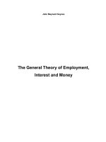
Example 1.1.3 Given a subset A ⊆ R, we define its indicator function χA : R → {0, 1} by

for x ∈ A,
 1
χA (x) =

0
for x ∈
/ A.

The indicator function is in some textbooks also called the characteristic function of the set A, and
denoted by 1A .
It follows from the above that A is a null set, if and only if χA is a null function.

Figure 2: The indicator function of Q ∩ [0, 1] is a null function, which is not Riemann integrable.

10
Download free eBooks at bookboon.com