DSpace at VNU: Regularization for the Inverse Problem of Finding the Purely Time-Dependent Volatility
Bạn đang xem bản rút gọn của tài liệu. Xem và tải ngay bản đầy đủ của tài liệu tại đây (503.34 KB, 18 trang )
Vietnam J. Math.
DOI 10.1007/s10013-015-0164-9
Regularization for the Inverse Problem of Finding
the Purely Time-Dependent Volatility
Dang Duc Trong1 · Dinh Ngoc Thanh1 ·
Nguyen Nhu Lan2
Received: 29 January 2014 / Accepted: 10 April 2015
© Vietnam Academy of Science and Technology (VAST) and Springer Science+Business Media Singapore
2015
Abstract We consider the inverse problem of finding the volatility σ ∈ Lρ (0, T ) such that
t
UBS (X, K, r, t, 0 σ 2 (τ )dτ ) = u(t), 0 ≤ t ≤ T , where UBS is the Black–Scholes formula
and u(t) is the observable fair price of an European call option. The problem is ill-posed.
Using the residual method, we shall regularize the problem. An explicit error estimate is
given.
Keywords Calibration · Volatility · Ill-posed · Regularization
Mathematics Subject Classification (2010) 35R30 · 65J20 · 91B24
1 Introduction
In the classical stochastic finance theory, the stock price X is assumed to satisfy an Ito
process (see [19, p. 13])
d X = μX dt + σ X dW,
where μ is the stock drift, σ = σ (t, X ) is the stock volatility, W is a Wiener process. Denote
by C(X, K, r, t, X ) the fair price of an European call option, where X is the current price of
the stock, K is the strike price, r is the continuously compounded interest rate, t is time. As
Nguyen Nhu Lan
1
Department of Mathematics and Computer Science, Ho Chi Minh City University of Science,
Vietnam National University, 227 Nguyen Van Cu, District 5, Ho Chi Minh City, Vietnam
2
Tay Do University, Can Tho, Vietnam
D.D. Trong et al.
shown by the Black–Scholes theory [21, p. 49], if the stock price X satisfies an Ito process
then the fair price C satisfies the (generalized) Black–Scholes equation
1
∂ 2C
∂C
∂C
+ X 2 σ 2 (t, X )
= 0.
+ rX
∂t
∂X
2
∂X 2
In the latter equation, the quantity σ (t, X ) plays a crucial role in option pricing. The volatility is used to measure the uncertainty of the future return of the stocks [20, p. 377]. If the
function is known, we can calculate the option price C(X, K, r, t, X ). The problem is called
the direct problem of option pricing.
However, the volatility σ (t, X ) is a market parameter and not directly observable. Hence,
it is also called the implied (or implicit) volatility. In the primitive Black–Scholes model,
the volatilities are assumed to be constants. However, in practice, the observation shows
that they are not constant over time. Therefore, the market is concerned with the problem of
identifying of non-constant volatility [20, p. 741]. We have the problem of calibrating the
implied volatility σ (t, X ) from the fair price of the option. It is called the inverse problem
of option pricing. The problem is ill-posed and studied in many papers [2–15, 18, 19, 24].
Among these papers, the method of integral equations (Green function) is used in [2–4, 19].
The mollification method is used in [12]. In other papers [7, 15, 18], the authors use the
Tikhonov method (or minimization method) to regularize the problem.
In the present paper, we deal with the case σ = σ (t). We put a(t) = σ 2 (t) and call it the
volatility function (see [14]). In this case, the dynamic of stock prices satisfies a generalized
geometric Brownian motion
d X = μX dt + σ (t)X dW.
We also note that similar purely t-dependent models can be seen in many papers. For
example, the value of an annually callable bond satisfies the Hull–White model
dr = (α(t) − β(t))r(t) + σ (t)dW.
If the stock prices are modeled by the generalized geometric Brownian motion then the
solution of the partial differential equation of C can be represented through the Black–
Scholes function [17, pp. 71–72]
XΦ(d1 ) − Ke−rt Φ(d2 ), s > 0,
s = 0,
(X − Ke−rt )+ ,
UBS (X, K, r, t, s) =
where ν = ln
X
K
and
ν + rt + 2s
,
√
s
√
1
Φ(z) = √
2π
Now, we can give a precise form of the inverse problem.
d1 =
d2 = d1 −
s,
z
−∞
e−x
2 /2
dx.
Calibration Problem Let u(t) be the known fair price of the market. We consider the
problem of finding the unknown volatility function a(t) from u(t) satisfying
t
UBS X, K, r, t,
a(τ )dτ
= u(t),
0 ≤ t ≤ T.
0
If we put for short
t
N0 (a)(t) = UBS X, K, r, t,
a(τ )dτ
0
then N0 is an operator N0 : a → N0 (a).
(1)
Regularization for the Inverse Problem of Finding the Purely...
The case of purely t-dependent volatility σ = σ (t) is studied only in a few papers as
[10, 14, 15, 23], especially, in [14, 23]. Since the problem is ill-posed, these papers studied
the regularization of the problem in many common spaces C[0, T ], L2 (0, T ), Lp (0, T )
(p ≥ 1). We will discuss the details later. From now on, we shall denote by uex the fair
price data, which is a function in the range of the operator N0 . Since N0 (a)(t) is increasing
with respect to t, the operator N0 is not surjective on the set of positive functions W =
C + [0, T ] ⊂ C[0, T ] or W = Lλ,+ (0, T ) = {v ∈ Lλ (0, T ) : v(x) ≥ 0 for x ∈ (0, T )}. Let
V be a normed space such that N0 (W ) ⊂ V . The problem of finding conditions of a datum
u ∈ V such that u ∈ N0 (W ) is called the problem of solvability. Moreover, in practical
situations, the exact datum uex is the result of a measurement. Hence, we often do not have
the exact value of the datum uex . We only get a noise uε such that
uε − uex
W
≤ ε.
The noise uε is often not in N0 (W ), i.e., the problem N0 (a) = uε possibly has no solution.
Therefore, the unsolvability often happens for real data. Even if uε ∈ N0 (W ), corresponding solutions might have large error (see the next section). Hence, the problem of stability
seems to be more important than the one of solvability. In the present paper, we only
consider the regularization for the problem.
We recall the definition of a regularization scheme in the present context. Since our
problem is nonlinear, we choose the classical definition in [22, Ch. 2, p. 43]. In fact, let
(U , · U ) and (Y , · Y ) be two normed spaces and A is an operator from U into Y with
A−1 : A(U ) → U not continuous. Let wex ∈ A(U ) be the exact datum, vex ∈ U be the
corresponding exact solution satisfying A(vex ) = wex and let wε ∈ Y be an inexact (but
real) datum of wex . From wε ∈ Y , we have to find a “stable solution” vε ∈ U (called a
regularization solution) for the problem. To this end, we consider some problems.
Let δ1 > 0 and O be a neighborhood of wex (in the topology of Y ). The first problem
is the one of convergence analysis (or consistency problem) which is of finding an operator
R : O × (0, δ1 ] → U , called a regularization scheme such that there exists a positive
function δ = δ(ε), limε→0+ δ(ε) = 0, satisfying
R(wε , δ(ε)) − vex
U
≤ε
for all wε ∈ O, wex − wε Y ≤ δ(ε).
As shown in [22, pp. 44–45], the latter property is fulfilled if two following properties
hold
(i)
(ii)
(continuous property) for each δ ∈ (0, δ1 ], R(·, δ) is continuous on O.
(inverse property) R(Av, δ) → v as δ → 0+ for every Av ∈ O.
The second problem is the one of convergence rate which is of establishing error estimate
between the regularization solution and the exact solution. As known, the problem is not
easy. Readers can see [16, 23] for some nontrivial estimates.
We turn to discuss our problem. In [14], the authors studied three versions: the C-space
case with U = Y = C[0, T ], the Lp -case with U = Lp (0, T ), Y = Lq (0, T ), and the L2 space case with U = Y = L2 (0, T ). As shown in the paper, in all cases, the problems are
ill-posed in the Hadamard sense [1, p. 17]. A regularization for the case U = Y = C[0, T ]
was not established in [14]. In [23], using an a priori information, the authors constructed a
regularization scheme for the continuous case. Moreover, they also considered the problem
D.D. Trong et al.
1
ε
of convergence rate for the C-space case and obtained the rate O ln
optimal in the sense that there exists a C0 > 0 satisfying
˜
R(w,
δ(ε)) − vex
sup
{w: wex −w Y <ε}
≥ C0 ln
U
1
ε
−1
. The rate is
−1
for every regularization R˜ and every function δ(ε) > 0 which has the property
limε→0+ δ(ε) = 0.
In the Lp -case, the authors of [14] considered only convergence analysis of regularization problem. Moreover, the regularization is descriptive. Hence, to get the consistency
result, a priori information in the solution was used. The authors studied the outer operator
N (S)(t) = UBS (X, K, r, t, S(t)) with S in the set
˜ 1 ) ≤ S(t
˜ 2 ) ≤ κ, t1 , t2 ∈ [0, T ], t1 < t2 .
Dκ+ := S˜ ∈ L∞ (0, T ) : 0 ≤ S(t
For a datum uδ ∈ Lq (0, T ), uδ (t) ≥ 0 (0 ≤ t ≤ T ), the authors found a minimizer S δ ∈ Dκ+
of the extremal problem
˜ − uδ
N (S)
Lq (0,T )
subject to S˜ ∈ Dκ+ .
→ min,
If N (S) = u and uδn → u in Lq (0, T ) then the authors proved that S δn → S in Lp (0, T )
as n → ∞. The problem of convergence rate was not studied in this case.
Finally, in the L2 -case, N0 is an operator in the Hilbert space L2 (0, T ). In [14], using the
Tikhonov method, the authors constructed the regularization solution aαδ as a minimizer of
the extremal problem
N0 (a)
˜ − uδ
2
L2 (0,T )
+ α a˜ − a ∗
2
L2 (0,T )
→ min,
subject to a˜ ∈ D(N0 ),
where a ∗ ∈ D(N0 ) is a fixed initial guess datum and
D(N0 ) := a˜ ∈ L2 (0, T ) : ess inf a˜ ≥ c0 > 0 .
0≤t≤T
The latter condition is crucial in the L2 -results of [14]. It was mentioned there “constraints
of the form a(t) ≥ 0 or 0 ≤ a(t) ≤ c < ∞ a.e. on [0, T ] are not able to stabilize the
solution process sufficiently”. Let L > 0 and G : L2 (0, T ) → L2 (0, T ) be the Fr´echet
derivative of N0 at a ∈ D(N0 ) such that
L
a˜ − a 2L2 (0,T ) .
2
From the√general theory of the Tikhonov regularization, to obtain the rate convergence of
order O( ε), we need [14, Proposition 5.3] the source condition
N0 (a)
˜ − N0 (a) − G(a˜ − a)
L2 (0,T )
≤
there exists a function w ∈ L2 (0, T ) satisfying a − a ∗ = G∗ w
and the closeness condition w
condition implies the condition
a − a ∗ ∈ H 1 (0, T ),
where m(t) =
∂UBS (X,K,r,t,S(t))
,
∂s
L2 (0,T )
<
1
L.
In the context of our problem, the source
a(T ) − a ∗ (T ) = 0,
(a − a ∗ )
∈ L2 (0, T ),
m
and the closeness condition has the form
(a − a ∗ )
m
<
L2 (0,T )
1
.
L
Regularization for the Inverse Problem of Finding the Purely...
Since the function a is unknown, it is not easy to find an initial guess datum a ∗ such that
a(T ) − a ∗ (T ) = 0 and that the other conditions hold.
In the present paper, we shall consider the problem of consistency and the problem of
convergence rate for the case U = Lλ (0, T ), Y = Lp (0, T ) (1 ≤ λ ≤ p < ∞). We note
that, in this case, Lp (0, T ) (p = 2) is not a Hilbert space, hence the standard Tikhonov
method (as in [14, 15]) could not be applied easily to solve the problem. Moreover, we also
−γ
give explicitly error estimates of order O ln 1ε
(γ > 0, see Corollary 1) in which we
do not use the strict conditions as σ (t) ≥ c0 > 0, the source condition and the closeness
condition. In the present paper, we do not obtain an optimal result for rate convergence. But,
from the optimal result in [23], the logarithmic rate in the present work is reasonable. We
will study the optimal rate convergence in a future work.
The remaining part of the paper is divided into five sections. In Section 2, we decompose
the problem into two problems called the outer and the inner ones, give some properties of
Black–Scholes formula and prove the instability of the inverse problems. Section 3 gives the
existence and the regularization of the outer problem. The regularization of whole problem
and rate of convergence are presented in Section 4. In Section 5, we give some numerical
experiments. Finally, we give conclusion of our paper in Section 6.
2 Preliminary Results
2.1 Some Properties of the Black–Scholes Formula
The following properties are presented in [23], but for convenience, we recall it here without
proofs. Since X, K, r are market observable constants, we can denote (for short)
k(t, s) = UBS (X, K, r, t, s).
The function UBS is defined in the domain X > 0, K > 0, r ≥ 0, t ≥ 0, s > 0. By direct
calculation, one has (see its proof, e.g., in [14])
(ν + rt)2
X
ν + rt
s
∂UBS
exp −
= √
−
−
∂s
2s
2
8
2 2π s
>0
and
lim UBS (X, K, r, t, s) = X,
s→+∞
lim UBS (X, K, r, t, s) = (X − Ke−rt )+ .
s→0+
From the latter limit, we shall put k(t, 0) = UBS (X, K, r, t, 0) := (X −Ke−rt )+ . We easily
get (see [23] for proofs)
Lemma 1 For t, s1 , s2 , s ≥ 0,
k(t, s1 ) < k(t, s2 ) if and only if 0 ≤ s1 < s2 . Hence, k(t, s1 ) = k(t, s2 ) if and only if
s1 = s2 .
b) (X − Ke−rt )+ ≤ k(t, s) < X.
c) If an α satisfies (X − Ke−rt )+ ≤ α < X then there exists uniquely a ξ(t) ≥ 0 such that
a)
k(t, ξ(t)) = α.
D.D. Trong et al.
Now, we consider the problem of finding a function S (Lebesgue) measurable on [0, T ]
such that k(t, S ) = ψ. The solution will be denoted by S = S(ψ).
From Lemma 1, we have
Proposition 1 Put
D = {v ∈ L∞ (0, T ) : (X − Ke−rt )+ ≤ v(t) < X a.e.}.
Let ψ : [0, T ] → R be a measurable function. The problem k(t, S ) = ψ has a unique
measurable solution S = S(ψ)(t) if and only if ψ ∈ D.
2.2 The Ill-posedness of the Calibration Problem
We shall consider the ill-posedness of N0 as an operator from Lλ (0, T ) to Lp (0, T ). Let
t
a0 ∈ Lλ (0, T ), u0 ∈ Lp (0, T ) satisfy N0 (a0 ) = u0 . Then k t, 0 a0 (τ )dτ = u0 (t). We
put un (t) = k t,
t
0 an (τ )dτ
where an (t) = a0 (t) + hn (t) and
hn (t) =
0, 0 ≤ t ≤ T − n1 ,
n3 , T − n1 ≤ t ≤ T .
For each t ∈ [0, T ), one has limn→∞ un (t) = u0 (t). From Lemma 1, one has 0 ≤ un (t) <
X. Using the Lebesgue dominated convergence theorem, one has
lim
n→∞
un − u0
p
= 0,
and
lim
n→∞
an − a0
λ
= hn
λ
= n2/λ = ∞.
This follows that the calibration problem is unstable at u0 . Hence, it is ill-posed.
2.3 The Outer and the Inner Problems
As mentioned in Introduction, the functions a(t), u(t), which satisfy the equation N0 (a) =
u, are called the exact solution and the exact data, respectively. Hence, we also denote
a = aex , u = uex . As shown in [14, 23], the problem can be divided into two problems.
The outer problem is
From a function u ∈ Y , we find a function S(u) : [0, T ] → [0, ∞) such that
k(t, S(u)(t)) = u(t)
and the inner problem is
From the solution of the outer problem S(u)(t), we find the (positive) volatility function
t
a(t) such that 0 a(τ )dτ = S(u)(t).
3 The Outer Problem
In the section, we shall construct a regularization scheme for the outer problem. The section
is divided into four subsections. In Section 3.1, we shall give a definition of the approximation R(w, δ) and compare with other regularization methods in [14, 23]. In the two
Sections 3.2, 3.3, we shall prove the consistency of our approximation. In fact, in Section 3.2, we shall prove that R(w, δ) satisfies the property (i), i.e., continuous with respect
to w, in the definition of regularization scheme in Introduction. The inverse property (ii)
is investigated in Section 3.3. Finally, in Section 3.4, we shall consider the problem of
convergence rate.
Regularization for the Inverse Problem of Finding the Purely...
3.1 Definition of Regularization Scheme for the Outer Problem
Let v ∈ Lλ,+ (0, T ) = {v ∈ Lλ (0, T ) : v ≥ 0}. We put
J (v)(t) = k(t, v(t)).
Let D be as in Proposition 1. As shown in Lemma 1, J : Lλ,+ (0, T ) → D ⊂ Lp (0, T ) is
injective. As noted in Section 1, for δ > 0, we shall construct R(·, δ) : D → Lλ,+ (0, T )
such that limδ→0+ R(J (v), δ) = v. In the section, we shall use the method of residuals
[1, p. 31] to regularize the outer problem. Hence, our regularization for (CP) can be called
a modified method of residuals. Precisely, let δ > 0 and let w ∈ D. Put
Bw,δ = {v˜ ∈ Lλ,+ (0, T ) ∩ L∞ (0, T ) : w − J (v)
˜
∞
≤ δ}.
From w, we construct a (minimizer) function R(w, δ) := ϕ such that ϕ ∈ Bw,δ and
ϕ(t) ≤ v(t)
˜
for every t ∈ [0, T ], v˜ ∈ Bw,δ .
(2)
The definition defines uniquely the function ϕ. We shall prove the existence of the minimizer. Before going to details of the construction, we have some comments. In [14],
the authors gave a result of convergence analysis for the outer problem in Lp -spaces. In
fact, with the datum w, they used the approximation R(w) as minimizer of the problem
J (v) − w Lq (0,T ) −→ min subject to
κ
= {v ∈ L∞ (0, T ) : 0 ≤ v(t1 ) ≤ v(t2 ) ≤ κ for 0 ≤ t1 ≤ t2 ≤ T }.
v ∈ D+
The algorithm depends on the constant κ which is an available a priori information.
As mentioned, the regularization is descriptive. Similarly, in [23], we used the formula
R(w, δ) = min{κ, max{S(w), δ}}. From the mathematical point of view, it might be better
if we have not to use the a priori constant κ. This is the reason of our algorithm.
Now, we give the closed-form of R(w, δ). Put
wδ+ (t) = max{(X − Ke−rt )+ , w(t) − δ}.
The definition of wδ+ implies wδ+ ∈ D. From Proposition 1, we can get the function S(wδ+ )
such that k(t, S(wδ+ )) = wδ+ . We shall prove that R(w, δ) = S(wδ+ ) in the following result
Lemma 2 Let δ > 0 and let w ∈ D. Then
i) S(wδ+ ) ∈ Bw,δ , S(wδ+ )(t) ≤ v˜ for every t ∈ [0, T ] and v˜ ∈ Bw,δ . Hence the function
S(wδ+ ) satisfies (2);
ii) Therefore, S(wδ+1 )(t) ≥ S(wδ+ )(t) for all t ∈ (0, T ) and 0 < δ1 < δ.
Proof We first prove S wδ+ ∈ Bw,δ . For every t ∈ [0, T ], we have 0 ≤ w(t) − wδ+ (t) ≤ δ
and
J (S(wδ+ ))(t) = k(t, S(wδ+ )(t)) = wδ+ (t).
+
So, w − J (S(wδ )) ∞ ≤ δ. It follows that S(wδ+ ) ∈ Bw,δ .
Now, we prove S(wδ+ )(t) ≤ v˜ for every v˜ ∈ Bw,δ . We have k(t, v(t))
˜
≥ w(t) − δ for all
t ∈ (0, T ). Lemma 1 implies k(t, v(t))
˜
≥ (X − Ke−rt )+ . Using both inequalities gives
k(t, v(t))
˜
≥ wδ+ (t) = k(t, S(wδ+ )(t))
˜ for all
for every t ∈ (0, T ). By the monotonicity of k(t, ·), we get 0 ≤ S(wδ+ )(t) ≤ v(t)
0 ≤ t ≤ T . This implies that S(wδ+ ) is a solution of (2).
Finally, we verify Part ii). In fact, we have
w − J (S(wδ+1 ))
∞
≤ δ1 .
D.D. Trong et al.
But 0 < δ1 ≤ δ, hence S(wδ+1 ) ∈ Bw,δ . From Part (i) of the lemma, we have S(wδ+ )(t) ≤
S(wδ+1 )(t) which gives the last desired inequality. This completes the proof of Lemma 2.
3.2 The Continuity of R(w, δ)
For a fixed δ, to prove the continuity of R(w, δ) with respect to w ∈ D, we state and prove
some lemmas.
Lemma 3 Let
√
2(X + K)
s ≥ m := max 2|ν|, 2|ν + rT |, 1 + max
,1 .
√
2π
Then there exists a positive number 0 < δ0 < 1 such that if the inequality k(t, s) ≤ X − δ
holds for a δ ∈ (0, δ0 ), then
2
1
8 ln
δ
m ≤ s ≤ Kδ ≡ 1 +
2
.
Proof We can rewrite the inequality k(t, s) ≤ X − δ as
X
√
2π
∞
e−t
2 /2
d1
∞
K
dt + √
2π
e−t
−d2
2 /2
dt ≥ δ.
Put β0 = max{|ν|, |ν + rT |}. We have for s ≥ m2 ≥ 4β02
√
√
β0
1
s
s
−√ ≥
− .
2
2
2
s
This implies
√
√
√
1
1
s
s
− , −d2 = −d1 + s ≥
− .
d1 ≥
2
2
2
2
So, we have
X+K ∞
2
e−t /2 dt ≥ δ.
√
√
s 1
2π
2 −2
Putting z =
√
s
2
− 12 , we have
∞
2 /2
dt =
z
It follows that
or
For
∞
e−z /2
−
z
2
e−t
2
z
X+K
X + K e−z /2
≥ √
√
z
2π
2π
∞
2
√
√
e−t /2
e−z /2
dt
≤
.
z
t2
2(X+K)
√
,1
2π
e−t
2 /8
8 ln
dt ≥ δ
≥ δ.
√
s−1)2 /8
, we shall get e−(
s ≤ 1+
2 /2
z
2(X + K)e−( s−1)
√
√
2π ( s − 1)
s ≥ m ≥ 1 + max
2
1
δ
≥ δ. This implies
2
.
By choosing δ0 > 0 small enough, we shall get the desired inequality for all 0 < δ ≤ δ0 .
This completes the proof of Lemma 3.
Regularization for the Inverse Problem of Finding the Purely...
Lemma 4 Let α, L satisfy 0 < α < L. For every s1 , s2 ∈ [0, L], one has
|s1 − s2 | ≤ α + M(α, L, t)|k(t, s1 ) − k(t, s2 )|,
where
√
(ν + rt)
s
2 2π s
(ν + rt)2
exp
+
+
α≤s≤L
X
2s
2
8
M(α, L, t) = max
and ν = ln
X
K
.
Proof We consider three cases.
Case 1 0 ≤ s1 , s2 ≤ α
|s1 − s2 | ≤ α ≤ α + M(α, L, t)|k(t, s1 ) − k(t, s2 )|.
Case 2 α ≤ s1 , s2 ≤ L.
We have k(t, s1 ) − k(t, s2 ) =
∂k
∂s (t, c)(s1
− s2 ), where
α ≤ min{s1 , s2 } ≤ c ≤ max{s1 , s2 } ≤ L.
Hence, 0 ≤
−1
∂k
∂s (c)
≤ M(α, L, t). This gives
|s1 − s2 | ≤ α + M(α, L, t)|k(t, s1 ) − k(t, s2 )|.
Case 3 0 ≤ s1 ≤ α ≤ s2 ≤ L.
One has
|s1 − s2 | = α − s1 + s2 − α
≤ α + M(α, L, t)|k(t, s2 ) − k(t, α)|.
But, from Lemma 1, one has k(t, s1 ) ≤ k(t, α) ≤ k(t, s2 ). This implies that |k(t, α) −
k(t, s2 )| ≤ |k(t, s1 ) − k(t, s2 )|. Hence,
|s1 − s2 | ≤ α + M(α, L, t)|k(t, s1 ) − k(t, s2 )|.
This completes the proof of Lemma 4.
Proposition 2 Let α be as in Lemma 4 and let δ > 0. For two functions u, w ∈ D one has
|S(u+
δ )(t)| ≤ Kδ = 1 +
2
8 ln 1δ
,
+
|S(u+
δ )(t) − S(wδ )(t)| ≤ α + M(α, Kδ , t)|u(t) − w(t)|
and
+
S(u+
δ ) − S(wδ )
λ
≤ αT 1/λ + max M(α, Kδ , t)T
0≤t≤T
p−λ
p
u−w
p.
As a consequence, R(·, δ) : D → Lλ (0, T ) is continuous. Here, we recall that D ⊂
Lp (0, T ) is defined in Proposition 1.
Proof For u, v ∈ Lp (0, T ) and t ∈ (0, T ) fixed, we give the estimate of
+
|R(u, δ)(t) − R(v, δ)(t)| = |S(u+
δ )(t) − S(vδ )(t)|.
D.D. Trong et al.
+
+
+
One has k(t, S(u+
δ )(t)) − k(t, S(vδ )(t)) = uδ (t) − vδ (t). For δ small enough, we obtain
+
+
0 ≤ uδ (t), vδ (t) ≤ X − δ. From Lemma 3, we shall get
0 ≤ S(u+
δ )(t),
S(vδ+ )(t) ≤ Kδ = 1 +
8 ln
1
δ
2
.
Using Lemma 3, one has
+
+
+
|S(u+
δ )(t) − S(vδ )(t)| ≤ α + M(α, Kδ , t)|uδ (t) − vδ (t)|.
+
On the other hand, |u+
δ (t) − vδ (t)| ≤ |u(t) − v(t)|. Hence,
+
|S(u+
δ )(t) − S(vδ )(t)| ≤ α + M(α, Kδ , t)|u(t) − v(t)|.
Now, we prove the continuity of R(·, δ). One has
+
|S(u+
δ ) − S(wδ )(t)| ≤ α + M(α, Kδ , t)|u(t) − w(t)|.
This implies
R(u, δ) − R(w, δ)
λ
≤ αT
1
λ
+ max M(α, Kδ , t)T
p−λ
p
u−w
0≤t≤T
p.
So, for wn ∈ D ⊂ Lp (0, T ) such that limn→∞ wn −w p = 0, we get after letting n → ∞,
α → 0 that lim supn→∞ R(wn , δ) − R(w, δ) λ = 0. It follows that R(·, δ) is continuous
at w ∈ D. This completes the proof of Proposition 2.
3.3 The Inverse Property of R(w, δ)
We shall prove that R(w, δ) is a regularization scheme. In fact, we prove
Proposition 3 Let vex ∈ Lλ,+ (0, T ). Then R(J (vex ), δ)(t) ↑ vex (t) as δ ↓ 0 and
lim R(J (vex ), δ) − vex
δ→0
λ
= 0,
where we recall that J (v)(t) = k(t, v(t)).
Proof Putting wex = J (vex ), we get wex ∈ D and vex = S(wex ). From the definition
+
+
of R, we have R(wex , δ) = S(wex,δ
). For 0 < δ1 < δ, Lemma 2 implies S(wex,δ
)(t) ≥
1
+
+
S(wex,δ )(t) for all t ∈ (0, T ). Hence, limδ↓0 S(wex,δ ) exists for every t ∈ (0, T ). Putting
+
+
), we claim that ψ = vex . In fact, wex − J (S(wex,δ
)) ∞ ≤ δ, by
ψ(t) = limδ↓0 S(wex,δ
Lemma 2. Let δ → 0, we get wex − J (ψ) ∞ = 0. This implies k(t, vex (t)) = k(t, ψ(t)).
Using Lemma 1, we get vex = ψ. Now, the Lebesgue monotone convergence theorem
implies
lim R(J (vex ), δ) − vex
δ→0
λ
This completes the proof of Proposition 3.
+
= lim S(wex,δ
) − vex
δ→0
λ
= 0.
Regularization for the Inverse Problem of Finding the Purely...
3.4 Error Estimates
We have
Proposition 4 Let L, ε, δ, α > 0 and let vex ∈ Lλ,+ (0, T ), wex = J (vex ). Let wε ∈ D be
such that wε − wex p ≤ ε. Then
1/λ
R(wε , δ) − vex
λ
≤ 2αT 1/λ +
{vex (t)>L}
+δ max M(α, L, t)T
|vex (t)|λ dt
p−λ
p
0≤t≤T
+ ε max M(α, Kδ , t)T
p−λ
p
0≤t≤T
.
So, if we choose δ
=
δ(ε), α
=
α(δ), L
=
L(δ) such that
limε→0 ε max0≤t≤T M(α, Kδ , t) = 0, limδ→0 α(δ) = 0, limδ→0 L(δ) = ∞, and
limδ→0 δM(α(δ), L(δ), t) = 0 for t ∈ (0, T ) then
lim R(wε , δ(ε)) − vex
λ
ε→0
= 0.
Proof We have
1/λ
R(J (vex ), δ) − vex
λ
≤
{vex (t)>L}
+
|vex (t)|λ dt
{0≤vex (t)≤L}
+
|S(wex )(t) − S(wex,δ
)(t)|λ dt
1/λ
.
+
)(t) ≤ vex (t) ≤ L. Hence, Proposition 2 gives
If 0 ≤ vex (t) ≤ L then 0 ≤ S(wex,δ
+
)| ≤ α + δM(α, L, t).
|S(wex )(t) − S(wex,δ
So,
{0≤vex (t)≤L}
+
|S(wex )(t) − S(wex,δ
)(t)|λ dt
1/λ
≤ αT 1/λ + δ max M λ (α, L, t)T
0≤t≤T
This implies
1/λ
R(J (vex ), δ) − vex
λ
≤
{vex (t)>L}
|vex (t)|λ dt
+αT 1/λ + δ max M(α, L, t)T
p−λ
p
0≤t≤T
.
On the other hand,
R(w, δ) − R(J (vex ), δ)
λ
+
= S(wδ+ ) − S(wex,δ
)
≤ αT
1/λ
λ
+
+ max M(α, Kδ , t) wδ+ − wex,δ
0≤t≤T
≤ αT 1/λ + max M(α, Kδ , t)εT
0≤t≤T
p−λ
p
.
λ
p−λ
p
.
D.D. Trong et al.
The above estimates give
1/λ
R(w, δ) − vex
λ
≤ 2αT 1/λ +
|vex (t)|λ dt
{vex (t)>L}
+δ max M(α, L, t)T
p−λ
p
0≤t≤T
+ ε max M(α, Kδ , t)T
p−λ
p
0≤t≤T
.
This completes the proof of Proposition 4.
We need an estimate for M(α, L, t). In fact, we have
Lemma 5 Put ν0 = max{|ν|, |ν + rt|}, K1 =
√
2 2π
X
exp
√
0 ≤ M(α, L, t) ≤ K1 L exp
ν0
2
. Then
ν0
L
+
.
2α
8
√
2
+ (ν+rt)
+
Proof We have M(α, L, t) = maxα≤s≤L 2 X2πs exp (ν+rt)
2s
2
t ≤ T , one has |ν + rt| ≤ max{|ν|, |ν + rT |} = ν0 . Hence,
√
ν02
2 2π L
ν0
L
0 ≤ M(α, L, t) ≤
exp
+
+
.
X
2α
2
8
s
8
. But, for 0 ≤
This completes the proof of Lemma 5.
Theorem 1 Let the assumptions of Proposition 4 hold. Let 0 < ρ < 1/2, δ = ε ρ . Put
V (L) = {vex > L} = {t ∈ (0, T ) : vex (t) > L}. Then there exist a constant C3 > 0 and
L = L(ε) > 0 such that limε→0 L(ε) = ∞ and
R(wε , δ) − vex
where
β(ε) =
⎧
⎪
⎪
⎨
⎪
⎪
⎩
Proof We choose α =
ν2
C3
+
ln 1ε
C3
ln 1ε
V (L(ε)) |vex (t)|
≤ β(ε),
λ dt
1/λ
if V (L(ε)) = ∅,
if V (L(ε)) = ∅.
C1
ln
λ
1
ε
, L = C2 ln
1
ε
, where the constants C1 , C2 > 0 satisfy
ν2
0 < 2C01 + 2r < 1, 2C01 + C82 < r. Using Proposition 4 and Lemma 5, we can compute
directly to get the desired estimate. This completes the proof of Theorem 1.
Corollary 1 Let the assumptions in Theorem 1 hold. If there exist μ, K2 > 0 such that
2
0 < λμ < 1 and 0 ≤ vex (t) ≤ (T K
−t)μ , then there exists a constant C4 > 0 such that
R(wε , δ) − vex
λ
C4
≤
ln
Proof The assumption on vex implies that L ≤
|vex (t)|λ dt ≤
vex (t)≥L
T
T−
K2
L
1/μ
1−λμ
λ
K2
(T −t)μ
1
ε
.
when vex (t) ≥ L. So, we have
K2λ
K2λ
dt =
λμ
(T − t)
−λμ + 1
K2
L
−λμ+1
.
Regularization for the Inverse Problem of Finding the Purely...
Direct computation gives the desired conclusion.
4 The Inner Problem
As mentioned, the inner problem is the one of recovering a derivative from its integral.
Precisely, we consider the problem of recovering the function aex (t) from the approximate
value Sε (t) = R(uε , δ(ε)) of Sex := S(uex )(t). The problem is ill-posed and many textbooks presented well-known regularization schemes. Here, we give only a simple version
t
of recovering the function aex (t). We recall that Sex (t) = 0 aex (τ )dτ . We first have
Lemma 6 Let 0 < h < 2h < T and let θ ∈ [0, h]. For f ∈ Lλ (0, T ), put
f (t + θ)
f (t − θ)
fθ (t) =
and ωf (h) = sup0≤θ≤h fθ − f
λ.
for 0 ≤ t ≤ T − h,
for T − h ≤ t ≤ T ,
Then limh→0+ ωf (h) = 0.
Proof Let ε > 0. Since C 1 [0, T ] is dense in Lλ (0, T ), there exists a continuous function
g ∈ C[0, T ] such that f − g λ ≤ 6ε . We note that
gθ − fθ
λ
λ
T −h
=
T
|g(t + θ) − f (t + θ)|λ dt +
T −h
0
T −h+θ
=
|g(t) − f (t)|λ dt +
θ
≤ 2 g−f
T −θ
|g(t − θ) − f (t − θ)|λ dt
|g(t) − f (t)|λ dt
T −h−θ
λ
λ.
Since λ ≥ 1, we have
gθ − f θ
λ
≤2 g−f
λ
+ g − gθ
λ.
Using the latter inequality, we have
f − fθ
λ
≤ f −g
λ
+ gθ − f θ
λ
≤ 3 f − g λ + g − gθ λ
1
≤ ε + ωg (h).
2
Since limh→0 ωg (h) = 0, we can find an h0 > 0 such that f − fθ
0 ≤ θ ≤ h ≤ h0 . This completes the proof of Lemma 6.
λ
≤ ε for every
Theorem 2 Let α0 ∈ (0, 1], 1 ≤ λ ≤ p and let the assumptions of Theorem 1 hold. In
addition, we assume that aex ∈ Lλ (0, T ). For h ∈ (0, T ) such that 0 < h < 2h < T , put
aεh (t) =
Sε (t+h)−Sε (t)
,
h
Sε (t)−Sε (t−h)
,
h
0 ≤ t ≤ T − h,
T − h < t ≤ T.
Then
aεh(ε) − aex
λ
≤ 31−1/λ 4T
p−λ
p
1/λ
(β(ε))(1−α0 )λ + 2ωaλex (β(ε))α0
,
where β(ε) is as in Theorem 1 and h(ε) = (β(ε))α0 . Moreover, if aex is a H¨older function
satisfying
|aex (t1 ) − aex (t2 )| ≤ K2 |t1 − t2 |γ
for t1 , t2 ∈ [0, T ],
D.D. Trong et al.
where 0 < γ ≤ 1, then we can choose α0 =
aεh(ε) − aex
λ
1
γ +1
≤ 31−1/λ 4T
to get
p−λ
p
1/λ
+ 2K2λ T
γ
(β(ε)) γ +1 .
If, in addition, we have the assumptions of Corollary 1 then
⎞ γ (1−λμ)
⎛
λ(1+γ )
1
h(ε)
⎠
⎝
.
aε − aex λ ≤ O
ln 1ε
Proof We have for 0 ≤ t ≤ T − h
|aεh (t) − aex (t)| ≤
1
(|Sε (t + h) − Sex (t + h)| + |Sε (t) − Sex (t)|)
h
1
+
|aex (t + hθ ) − aex (t)|dθ.
0
a+b+c λ
3
Using the inequality
T −h
0
≤
a λ +bλ +cλ
3
for a, b, c ≥ 0, λ ≥ 1, we get
|aεh (t) − aex (t)|λ dt ≤ I1 + I2 + I3 ,
where
3λ−1
hλ
3λ−1
I2 =
hλ
T −h
I1 =
|Sε (t + h) − Sex (t + h)|λ dt ≤
0
T −h
|Sε (t) − Sex (t)|λ dt ≤
0
T −h
I3 = 3λ−1
0
1
0
p−λ
p
p−λ
p
β λ (ε),
β λ (ε),
λ
|aex (t + hθ ) − aex (t)|dθ
dt ≤ 3λ−1 ωλ (h).
0
The estimates of I1 , I2 , I3 imply that
T −h
3λ−1
T
hλ
3λ−1
T
hλ
⎛
|aεh (t) − aex (t)|λ dt ≤ 3
λ−1 ⎝ 2T
p−λ
p
⎞
β λ (ε)
hλ
+ ωaλex (h)⎠ .
Similarly, for T − h < t ≤ T , we have
|aεh (t) − aex (t)| ≤
1
(|Sε (t) − Sex (t)| + |Sε (t − h) − Sex (t − h)|)
h
1
+ |Sex (t) − Sex (t − h) − haex (t)|.
h
It follows that
⎛
T
T −h
|aεh (t) − aex (t)|λ dt
≤3
We get in view of the above inequalities
T
0
|aεh (t) − aex (t)|λ dt ≤ 3
λ−1 ⎝ 2T
⎛
λ−1 ⎝ 4T
p−λ
p
⎞
β λ (ε)
hλ
p−λ
p
+ ωaλex (h)⎠ .
⎞
β λ (ε)
hλ
+ 2ωaλex (h)⎠ .
Regularization for the Inverse Problem of Finding the Purely...
By choosing h = h(ε) = (β(ε))α0 , we get
T
0
|aεh(ε) (t) − aex (t)|λ dt ≤ 3λ−1 4T
p−λ
p
(β(ε))(1−α0 )λ + 2ωaλex (β(ε))α0 ) .
Since aex is in Lλ (0, T ), Lemma 6 gives
lim ωaex (h) = 0.
h↓0
Noting that β(ε) → 0 as ε → 0, we get the desired result.
Moreover, if aex is a H¨older function as in the statement of the theorem then
|aex (t1 ) − aex (t2 )| ≤ K2 |t1 − t2 |γ ≤ K2 hγ ,
In this case, we have |(aex )θ (t) − aex (t)| ≤ K2
T
0
|θ |γ .
t1 , t2 ∈ [0, T ], |t1 − t2 | ≤ h.
It follows that
|(aex )θ (t) − aex (t)|λ dt ≤ K2λ T |θ |λγ .
Therefore,
ωaλex (h) ≤ sup
T
0≤θ≤h 0
So, if α0 =
1
1+γ
1
, h = (β(ε)) γ +1 then
T
0
|aθ (t) − a(t)|λ dt ≤ K2λ T hλγ .
|aεh(ε) (t) − aex (t)|λ dt ≤ 3λ−1 4T
p−λ
p
+ 2K2λ T
λγ
(β(ε)) γ +1 .
This implies
aεh(ε) − aex
λ
≤ 31−1/λ 4T
p−λ
p
1/λ
+ 2K2λ T
γ
(β(ε)) γ +1 .
Now, if we have the assumptions of Corollary 1, then we can choose β(ε) =
ln
C4
1−λμ
λ
1
ε
to
get the final result. This completes the proof of Theorem 2.
Table 1 Error between exact solution and approximate solution
ε = 10−2
ti
ε = 10−3
Error
ti
ε = 10−4
Error
ti
Error
0
0.02703
0
0.00752
0
0.00778
0.25000
0.03922
0.16667
0.04076
0.12500
0.02793
0.50000
0.06152
0.33333
0.03171
0.25000
0.02713
0.75000
0.03585
0.50000
0.03505
0.37500
0.02725
0.66667
0.04647
0.50000
0.02914
0.83333
0.03926
0.62500
0.02785
0.75000
0.02820
0.87500
0.03222
D.D. Trong et al.
5 Numerical Results
From the results of the previous sections, we have many ways to establish a computation
program. Here, we give a rough algorithm. The given data are K, X, r, T , the noise level ε,
and the noise fair option price u(t). Since u ∈ D (see Proposition 1), we can replace u by
min{u, X}. The algorithm is divided into three steps.
Step 1 We can choose h = h(ε) = β(ε) ∼ O
1
ln
1
ε
as in Theorems 1 and 2. We divide
the interval [0, T ] into n subintervals by ti = (i − 1)T /n, i = 1, . . . , n + 1, where
T
.
n := β(ε)
Step 2 We construct the function R(u, δ)(t) for t = ti , 1 ≤ i ≤ n + 1. Let δ = δ(ε) =
ε ρ be as in Theorem 1. We can find Si := R(u, δ)(ti ) by solving the equation
k(ti , x) = max{(X − Kerti )+ , u(ti ) − δ} (i = 1, . . . , n + 1).
Step 3 We denote
ai =
Si+1 − Si
n
= (Si+1 − Si )
ti+1 − ti
T
for i = 1, . . . , n.
The output is an approximation of the implied volatility a(t) at ti = (i − 1)T /n,
i = 1, . . . , n + 1, i.e., (a(t1 ), . . . , a(tn+1 )) ≈ (a1 , . . . , an+1 ).
For example, we choose T = 1, X = 100, K = 101, r = 0.05 and a volatility function
a(t) = 0.2 +
0.02
.
(1 − t)0.1
We use blsprice (Price, Strike, Rate, Time, Volatility) in MATLAB R2013a to calculate
u(ti ). Testing with ε = 10−2 , 10−3 , 10−4 and error at points ti is as Table 1. In Figs. 1 and
2, we plot the exact solution and the approximate solution. In left panels, the graph of exact
outer solution is blue and the graph of approximate outer solution is green. Right panels are
graphs of exact (red) and approximate (blue) volatility functions.
(a) Outer solution
Fig. 1 ε = 10−3
(b) Volatility function
Regularization for the Inverse Problem of Finding the Purely...
(a) Outer solution
(b) Volatility function
Fig. 2 ε = 10−4
6 Conclusion
The regularization problem of finding a purely time-dependent volatility is considered in
a lot of papers [14–16, 23]. Our paper is devoted to the Lp -case of the problem. In [14],
the authors considered the case and established the convergence analysis for a descriptive
regularization with p = 2. But the regularization needed an available a priori constant,
and the rate of convergence was not considered. Now, in our paper, we construct a regularization scheme in which we do not use the a priori constant. We also give an analysis for
convergence rate of our regularization and some numerical experiments.
Acknowledgments The authors are grateful to three anonymous referees for their precious suggestions
leading to the improvement version of our paper.
References
1. Baumeister, J.: Stable solution of inverse problems. Friedr. Vieweg & Son (1987)
2. Bouchouev, I., Isakov, V.: The inverse problem of option pricing. Inverse Probl. 13, L11–L17 (1997)
3. Bouchouev, I., Isakov, V.: Uniqueness, stability and numerical methods for the inverse problem that
arises in financial markets. Inverse Probl. 15, R95–R116 (1999)
4. Bouchouev, I., Isakov, V., Valdivia, N.: Recovery of volatility coefficient by linearization. Quant. Financ.
2, 257–263 (2002)
5. Chargory-Corona, J., Ibarra-Valdez, C.: A note on Black–Scholes implied volatility. Phys. A 370, 681–
688 (2006)
6. Cr´epey, S.: Calibration of the local volatility in a generalized Black–Scholes model using Tikhonov
regularization. SIAM J. Math. Anal. 34, 1183–1206 (2003)
7. De Cezaro, A., Scherzer, O., Zubelli, J.P.: Convex regularization of local volatility models from option
prices: convergence analysis and rates. Nonlinear Anal. 75, 2398–2415 (2012)
8. Deng, Z.-C., Yu, J.-N., Yang, L.: An inverse problem of determining the implied volatility in option
pricing. J. Math. Anal. Appl. 340, 16–31 (2008)
9. Egger, H., Engl, H.W.: Tikhonov regularization applied to the inverse problem of option pricing:
convergence analysis and rates. Inverse Probl. 21, 1027–1045 (2005)
10. Egger, H., Hein, T., Hofmann, B.: On decoupling of volatility smile and term structure in inverse option
pricing. Inverse Probl. 22, 1247–1259 (2006)
11. Engl, H.W., Zou, J.: A new approach to convergence rate analysis of Tikhonov regularization for
parameter identification in heat conduction. Inverse Probl. 16, 1907–1923 (2000)
12. Guo, L.: The mollification analysis of Stochastic volatility. Actuar. Res. Clear. House 1, 409–419 (1998)
D.D. Trong et al.
13. Hein, T.: Some analysis of Tikhonov regularization for the inverse problem of option pricing in the
price-dependent case. Z. Anal. Anwend. 24, 593–609 (2005)
14. Hein, T., Hofmann, B.: On the nature of ill-posedness of an inverse problem arising in option pricing.
Inverse Probl. 19, 1319–1338 (2003)
15. Hofmann, B., Kr¨amer, R.: On maximum entropy regularization for a specific inverse problem of option
pricing. J. Inverse Ill-Posed Probl. 13, 41–63 (2005)
16. Kr¨amer, R., Math´e, P.: Modulus of continuity of Nemytskii operators with application to the problem of
option pricing. J. Inverse Ill-Posed Probl. 16, 435–461 (2008)
17. Kwok, Y.-K.: Mathematical models of financial derivatives. Springer, Berlin–Heidelberg (1998)
18. Lishang, J., Youshan, T.: Identifying the volatility of underlying assets from option prices. Inverse Probl.
17, 137–155 (2001)
19. Lu, L., Yi, L.: Recovery implied volatility of underlying asset from European option price. J. Inverse
Ill-Posed Probl. 17, 499–509 (2009)
20. McDonald, R.L.: Derivatives markets. Addison Wesley (2006)
21. Roberts, A.J.: Elementary calculus of financial mathematics. SIAM, Philadelphia (2009)
´
22. Tikhonov, A., Ars´enine, V.: M´ethodes de r´esolution de probl`emes mal pos´es. Edition
Mir (1974)
23. Trong, D.D., Thanh, D.N., Lan, N.N., Uyen, P.H.: Calibration of the purely T-independent Black–Scholes
implied volatility. Appl. Anal. 93, 859–874 (2014)
24. Zang, K., Wang, S.: A computational scheme for uncertain volatility model in option pricing. Appl.
Numer. Math. 59, 1754–1767 (2009)