DSpace at VNU: An efficient ant colony optimization algorithm for multiple graph alignment
Bạn đang xem bản rút gọn của tài liệu. Xem và tải ngay bản đầy đủ của tài liệu tại đây (283.47 KB, 6 trang )
An Efficient Ant Colony Optimization Algorithm
for Multiple Graph Alignment
Tran Ngoc Ha
Do Duc Dong, Hoang Xuan Huan
Thai Nguyen University of Education,
Vietnam National University - Hanoi,
,
Abstract - The Multiple Graph Alignment (MGA) is a new
method to analyze the structure of biological molecules. This
method allows detect functional similarities in the structure of
biological systems. This article introduces an ant colony
optimization algorithm combined with local search for
optimal align multi-graph analysis of protein structures.
Experiment results showed that the new algorithm
outperformed the other heuristic approach and existing
evolutionary computing.
evolutionary algorithm called GAVEO. Experiments show
that it is more efficient than the greedy algorithm.
For NP-hard problems, there were many natural
simulation approaches to find approximate solutions. In
particular, the experiments showed that the ant colony
optimization (ACO) method is better than evolutionary
algorithms in many typical problems [3, 4, 7]. This article
introduces an ant colony optimization algorithm
incorporating local search to aligning the multi-graph
called ACO-MGA. The simulation results show that ACOMGA algorithm is more outstanding effective than the
GAVEO and Greedy algorithms.
Keyword -Multiple Graph Alignment, label, Ant Colony
Optimization, Local Search, Pheromone update rule
I. INTRODUCTION
The multiple graph alignment techniques [14] are a
useful tool to analyze the similarity of DNA sequences or
proteins, thereby we can detect the similarity of different
molecules based on genetics. However, the functional
similarities among the genes and proteins are closely
related to the structure rather than sequential features [5.13]
so it is necessary to develop new research approaches.
The rest of this article is organized as follows: Section
2 mathematic defines the MGA problem and introduces the
schema of ACO method. New algorithm is introduced in
Section 3, the experiment results which comparing the new
algorithm with the GAVEO and Greedy algorithm are
presented in Section 4. The conclusions are presented in the
last section.
There have been different proposed approaches to
explore the structure similarities (see [2, 8-13, 16-18]), that
mainly due to correct graphs matching technique and get
the meaningful results when studying the functional
evolution of heterogeneous molecules. However, these
methods are difficult to discover biological meaningful
patterns that are stored approximately.
II. MULTIPLE GRAPH ALIGNMENT PROBLEM
AND RELATED WORKS
A. Multiple graph alignment problem
Weskamp et al. [15] proposed using the MGA problem
to study protein characteristics, where graphs are used to
approximately describe the binding pockets. This approach
is extended to analysis structure of biological molecules
which include chemical compounds and protein binding
sites by Fober et al [5]. Mathematical definition of MGA
problem is as follows (more details see [5]).
Weskamp et al [15] firstly introduced the concept of
multigraph alignment (MGA) in 2007; they used it to
analyze protein active sites, and proposed a heuristic
algorithm to find greed-based solutions. In this approach,
each binding pocket is modeled by a connected graph G(V,
E) and the MGA problem is defined as follows. Given a set
of connected graphs G = {G1(V1, E1), ..., Gn(Vn, En)}, each
vertex is labeled in a given label set and the weighted
edges; in each graph, there are four operations: deleting a
node, inserting a node, changing a label of a node and
changing the weight of an edge. Task of the MGA problem
is aligning the nodes of the graphs in the set G to optimize
a predefined objective function.
Multigraph
Multigraph
is
a
set
of
graphs
G
=
{G1(V1,E1),…,Gn(Vn,En)}, where the graphs Gi(Vi,Ei) are
connected graphs, node is labeled under a given set L, the
weighted edges represent the distance between the vertices.
In the model of protein binding sites, the labels of the nodes
can be: hydrogen-bond donor, acceptor, mixed
donor/acceptor, hydrophobic aliphatic and aromatic. In
each graphs, there are edit operations which is mathematic
defined as follow:
MGA is the NP-hard problem (see [5.15]), the
heuristic algorithms is only suitable for small size
problems, so it is not suitable for real applications. Fober et
Definition 1. On the graph G(V, E) of multigraph G
there are edit operations:
al [5] have extended the use of this problem for the
structural analysis of biomolecules and have proposed an
978-1-4673-2088-7/13/$31.00 ©2013 IEEE
386
i)
ii)
iii)
Insertion or deletion of a node: A node v ∈ V and
all relationships with it (edges) can be deleted or
inserted
Change of the label of a node: The label ݈ሺݒሻ of a
node ܸ ∈ ݒcan be changed by another label in
set L.
Change of the weight of an edge: The weight w(e)
of an edge e ∈ E can be changed depending on the
different forms.
n
s ( A) = ∑ ns ( a i ) +
i =1
∑
es( a i , a j )
(1)
1≤ i < j ≤ n
Where ns is the assessment score of the suitability of
the corresponding column and calculated by the expression
(2):
nsm
a
nsmm
ns M = ∑
a i 1≤ j < k ≤ m nsdummy
m
nsdummy
i
1
Multiple Graph Alignments
Give multigraph G ={G1(V1,E1),…,Gn(Vn,En)}, for each
vertex sets Vi , we add to it a dummy node (denoted ⊥) that
is not connected to the other nodes, an alignment of G is
defined as follows.
l(a ij )=l(aki )
l(a ij ) ≠ l(aki )
(2)
a ij = ⊥ , aki ≠⊥
a ij ≠⊥ , aki =⊥
and es evaluate the compatibility of the edge length and
is calculated by the expression (3):
Definition 2. (Multigraph Alignment).
Set { ⊆ܣV1 ∪ ሼ⊥ሽ} × … × {Vm ∪ ሼ⊥ሽ} is an alignment of
multigraph G if and only if it verifies two conditions:
esmm
(aki ,akj ) ∈ Ek , (ali ,alj ) ∉ El
a1i a1j
(aki ,akj ) ∉ Ek , (ali ,alj ) ∈ El
esmm
es M , M = ∑
d klij ≤ ε
(3)
ai a j 1≤ k
es
ij
d
>
ε
mm kl
1. For all i=1,…,n and for ܸ ∈ ݒ , there exists exactly
one a = (a1,…,an) ∈ ܣsuch that ݒൌ ܽ
2. For each a = (a1,…,an) ∈ ܣ, there exists at least
one 1 ≤ i ≤ n such that ܽ ് ⊥
In the expression (3) ݀ ൌ หݓ൫ܽ ൯ െ ݓ൫ܽ ൯ห. Five
parameters (nsm, nsmm, nsdummy, esm, esmm) are reused as
[15]: nsm = 1.0; nsmm = -5.0; nsdummy = -2.5; esm = 0.2; esmm
=-0.1.
Fig. 1 shows an alignment of four graphs, where
dummy nodes are presented by square, labeled nodes are
presented by circular. Noting that in each graph, there is
only one dummy node, but for ease of visualization, in the
first and the fourth graph there are two dummy nodes, that
means the nodes in the corresponding row are aligned with
dummy nodes in these graphs.
The solution of MGA problem is an alignment that
maximizing scoring function ݏሺܣሻ.
This problem is NP-hard (see [5.15]), the complexity of
algorithms is very large, for example, if you use an
exhaustive method, the complexity is O(ሺܸ݉ܽݔሻ! ) with
Vmax is the number of vertices of the graph that there is
maximum node and m is the number of graphs. Weskamp
et al. [15] introduced the greedy algorithm; it transforms
the comparing of multiple graphs become the problem of
comparing two graphs to find a solution that is good
enough to solve the problem in a short time. Fober et al [5]
proposed genetic algorithms called GAVEO significantly
improve performance compared with the greedy algorithm,
although it runs in a longer time.
Fig. 1: A multiple graph alignment of the four graphs, the node labels are
indicated by the letters assigned to the nodes (presented by circles) and
dummy nodes are indicated by squares.
B. Ant Colony Optimization method
To assess the quality of an alignment, we use the
scoring function for the edit distance. This function is
defined based on the set of edit operations mentioned above
to match the pairwise graphs followed the selected
alignment.
ACO method had been proposed by Dorigo in 1991
(see [4]). Until now, it had been developed into many
variations to solve hard combinatorial optimization
problems. In these algorithms, the under-examined problem
is transformed into the path finding problem on a
construction graph G= (V,E,Ω, η,T), where V is a set of
vertices, E is a set of edges, Ω is a set of constraints for
solution building, η and T is the vectors that denotes
heuristic information and reinforcement learning
information for solution finding (their elements can be on
the vertices or on the edges).
For ease of presentation, in the rest of the article we
keep the notation convention G ={G1(V1,E1),…,Gn(Vn,En)}
to refer to the multigraph in which the graph Gi has
additional dummy node Vi for all i=1,…,n.
The scoring function for alignment quality
Define 3(Scoring function)
In each iteration, each ant in the m ant colony will
build the solution on the Construction graph from a starting
set C0 and randomly sequential develop based on
reinforcement learning information at pheromone trail and
For each alignment matrix A of multigraph G, the
scoring function s(A) is defined as (1):
387
heuristic information follow random walk procedure
satisfy the constraints Ω. Then, those solutions are
evaluated and used for updating the pheromone trails as
reinforcement learning information that helps ant colony
constructs solutions in the next loops, more details see [4].
This procedure is specified in Fig. 2.
specially, the dummy nodes allow many lines passed
through it. The set of these paths can be seen as an only
path as the concept of the common ACO algorithm with
indicates that this line starts from a node of G1, passes
through the next graphs, when reaching to the first or the
last layer, "walking" to the other node on the same layer
and return back until through every node exactly once time.
Procedure of ACO algorithms;
Begin
Initialize; // initialize pheromone trail matrix and u ants
Repeat
Construct solutions;
// each ant constructs its own
solution
Improve solutions by local search // if it’s necessary
Update trail;
Until End condition;
End;
Random Walk Procedure to build an alignment
In each iteration, each ant will perform iterative
process to buil the vectors a = (a1,…,an) for an alignment A
as follows:
Ants randomly select a real node on the construction
graph and based on the heuristic information and the
pheromone trail to randomly walk to build a solution. For
ease of envisioning, we assume that this real node is in G1
(denoted as a1), ants will randomly walk across the layers to
Gn as follows. If ants have built vectors
(a1,…,ai) where aq is the vertex j of Gi then selected node k
in Gi +1 with probability given by Equation (4)
Fig. 2. Specification of an ACO algorithm
To apply ACO method, there are three factors that need
to be resolved: 1) the construction graph and sequential
developed procedures according to given constrains, 2)
heuristic information, 3) pheromone update rule. Below, we
introduce an ACO algorithm for the MGA problem called
as ACO-MGA
ఛೕ,ೖ
כቂఎೕ,ೖ
ሺሻቃ
α
Pkij =
III. ACO-MGA ALGORITHM
β
α
ఛ כቂఎೕ,ೞ
ሺሻቃ
శభ ೕ,ೞ
∑ೞചೃ_ೇ
β
(4)
where R_Vi is the number of remaining un-aligned
nodes on Vi included dummy node, ߬,
is intensity of
pheromone trail of the edge connected vertex j of Gi with
vertex k of Gi+1 , and ߟ,
ሺܽሻ is heuristic information
calculated by Eq (5).
Considering the alignment problem for multi-graph G
={G1(V1,E1),…,Gn(Vn,En), after the addition of the dummy
node to the vertices set of the graph Gi as mentioned above,
the Construction Graph and the solution building procedure
as follows.
ேሺ,ሻ
ሺܽሻ ൌ ቊ
ߟ,
Construction Graph
th
Construction Graph consists of n layer, the i layer is
the graph Gi of G, the vertices of the upper layer connect to
all nodes of the lower one. Fig. 3 shows the construction
graph, where the edges of each graph in each layer aren’t
showed, the circles are real node and dummy nodes are
represented by a square.
ߟ
݇ ݅݁݀݊ ݈ܽ݁ݎ ܽ ݏ
݇ ݅ݕ݉݉ݑ݀ ݏ
(5)
where NL(k,a) is the number of vertexs in {a1,…ai}
that its label is like the label l(k) of vertex k, ߟ 0 is
given enough small value.
After vector a is developed to a=(a1,…an), the real
vertices in a is removed from the construction graph to
continue repeating the alignment procedure of ants until
every vertex has been aligned. The alignment process of
ants is illustrated in Fig. 4, where the dummy nodes are
numbered -1, the other nodes are numbered 0, 1, 2,...
Noting that if the real node which is original selected is
not on the G1, it is on Gm, the above procedures can be
divided into two processes aligning from Gm to Gn and
aligning backwards from Gm to G1
Fig. 3. The construction graph of n graphs alignment where each graph
contains 2 or 3 nodes
An alignment of the graph in defined 2 above is a path
from G1 through all the layers to Gn layer such that each
line passes through a node of each layer and each node of
construction graph there is exactly one line passed through,
388
IV. EXPERIMENT RESULTS
Experiments to compare the ACO-MGA with Greedy
algorithm [15] and the evolution algorithm called GAVEO
[5] on the solution quality and runtime:
1) Run algorithms with the same data sets and a
predefined number of loops to compare the effect and
runtime.
2) Run algorithms with the same data sets with the
same predefined time to compare scoring of the alignment.
The experiments are performed on a computer with:
CPU Dual Core 2.2 Ghz, RAM DDR3 3GB running
Windows XP SP3. We run each of the three algorithms 10
times and compare the average results. The parameters had
been set as follows:
•
•
•
Fig. 4. Ant builds the solution
Pheromone Update Rule
After the ants have found the solution, the solutions of
iteration are evaluated and selected the best solution to
perform local search to improve quality then perform
pheromone trail updating.
SMMAS Pheromone Update Rule is applied as in [2] and
[6], detail as follow:
߬ ՚ ሺ1 െ ߩሻ߬ ∆
(6)
ߩ߬௫ ሺ݅, ݆ሻܾ߳݁݊݅ݐݑ݈ݏ ݐݏ
where: ∆ ൌ ൜
(7)
ߩ߬
݁ݏ݅ݓݎ݄݁ݐ
τmax and τmin is predefined parameter.
The number of ants in each loop is 20
ρ=0.6, ߙ ൌ ߚ ൌ 1
τmax = 1.0 và τmin = τmax/(n2*Vmax2), where n is the
number of graph, Vmax is the number of node of
the graph that has the most node.
Because there is no real data, we use Graph Generator
program to generate data as in [5] where each graph has 20
or 50 vertices and the number of graph alternately is 4, 8,
16 and 32.
A. Effect and Runtime comparisons
Table 1 and table 2 below are the results of comparing
the method about score and runtime. Table 1 is the result of
the alignment of the graphs has average 20 vertices and
table 2 results of the alignment of graphs with an average
of 50 vertices. The best score are shown in bold.
Local search
Table 1. Comparison of the score and runtime with the data sets
including 4, 8, 16 and 32 graphs, and the average number of the vertices of
each set is 20 nodes
Method/Number of
4
8
16
32
graphs
Local search procedure is applied to the best solution
by principles better then stopped. In this procedure, the pair
of the same label vertices in each graph Gi which is
randomly selected will be swapped in the its alignment
vector to improve the suitability of the weights of the
relevant edges. If after swapped, scoring function is
increasable, the getting solution will replace the best
solution and stop the search procedure of iteration to update
the pheromone.
Greedy
GAVEO
ACO-MGA
A permutation of the two node labeled A is illustrated
in Fig. 5, where alignment vectors are column vectors; the
letters are the label of the corresponding components.
Score
-40
-35
-570
-1055
Time
0.6
2.3
6
17
Score
-20
65
45
1132
Time
Score
249
123.8
501
696.1
1087.7
1479.7
2484.1
7288.5
Time
33.6
231.5
481.2
1266
Table 2. Comparison of the score and runtime with the data sets including
4, 8, 16 and 32 graphs, and the average number of the vertices of each set
is 50 nodes
Method/Number of
4
8
16
32
graphs
-1144
-4704
-31004
-155508
Score
Greedy
4.8
11.3
49
210.8
Time
-101
-75
-10872
-33698
Score
GAVEO
1164
2739.1
6921.3
16340.8
Time
Score
684.9
3337.6
1273.1
-18642.9
ACO-MGA
763.4
6523.5
12670.5
28859.8
Time
Fig. 5. A permutation of the two same label nodes in Local Search
procedure
Comment. The experimental results show that:
• In the two cases the graphs have average 20 vertices
or 50 vertices, the runtime of Greedy algorithms is
very little than the other two algorithms. However,
the results of this algorithm are very low in
comparison to GAVEO and ACO-MGA.
ACO-MGA algorithm performs as specified in Fig. 2
for the case of apply local search procedure.
389
TABLE 8. Comparison of results of ACO-MGA algorithm and GAVEO
algorithm with data sets consist of 4,8,16 and 32 graphs, with the average
number of vertices of each graph is 50 vertices and runtime is 600s
Method/Number of
4
8
16
32
graphs
GAVEO
-107
-77
-5282
-96123
Score
ACO-MGA Score
672.9
2898.4
744.8
-16945.8
• The ACO-MGA algorithm results better algorithm
GAVEO more. With the graphs have average 20
vertices, the runtime of ACO-MGA is faster than
GAVEO but when the number of vertices in the
graphs increases, the runtime of GAVEO is faster in
case the number of graph is over 4. However, the
experiments in the next section shows in the same
running time, the ACO-MGA still give much better
score than GAVEO.
The comparison of score of ACO-MGA algorithm and
GAVEO algorithm on data sets consist of 32 graphs with
the average number of vertices of each graph is 20 vertices
when increasing time from 50s to 200s is as fig.6.
B. Comparing evolution algorithm and ACO-MGA
algorithm in the same runtime
Since Greedy algorithm has short runtime, but it has
low score, in this article we only conducted experiments to
compare the performance of evolutionary algorithms and
the ACO-MGA algorithm with the same runtime. The
experiments performed on the same data set and the same
runtime to compare the score of two algorithms.
First experiment, running on the data sets consist of 8,
16 and 32 graphs, each graph has average of 20 vertices
and runtime alternately is 50s, 150s and 200s. Experimental
results are shown in Table 3, Table 4 and Table 5.
The second experiment, run on data sets consist of 4, 8,
16 and 32 graphs, each graph has average of 50 nodes and
runtime alternately is 200s, 300s and 600s. The results of
this experiment are presented in Tables 6, 7 and 8. The
better results shown in bold.
Fig. 6. Comparison of results of ACO-MGA algorithm and GAVEO
algorithm with data sets consist of 32 graphs, with the average number of
vertices of each graph is 20 vertices and runtime is 50,150 and 200s
Comment. The above results showed that in the same
runtime, the new algorithm gives much better results than
GAVEO
TABLE 3. Comparison of results of ACO-MGA algorithm and GAVEO
algorithm with data sets consist of 8, 16 and 32 graphs, with the average
number of vertices of each graph is 20 vertices and runtime is 50s
Method/Number of
8
16
32
graphs
57
46
-1327
GAVEO
Score
ACO-MGA
Score
689.1
2004.1
6511.2
V. CONCLUSION
MGA problem is a new approach to analysis the
structure of biological molecules, so far there have been
two commonly algorithms solved it. Greedy algorithm is a
heuristic algorithm, so it is outstanding in runtime but not
effective.
TABLE 4. Comparison of results of ACO-MGA algorithm and GAVEO
algorithm with data sets consist of 8, 16 and 32 graphs, with the average
number of vertices of each graph is 20 vertices and runtime is 150s
Method/Number of
8
16
32
graphs
GAVEO
75
35
953
Score
ACO-MGA
Score
689.7
2180.9
7166.1
Our new algorithms called ACO-MGA has much
better results than GAVEO when run on the same data set
and the same runtime. When the number of vertices of the
graph increases, the duration of local search in ACO-MGA
also increases, so the runtime of ACO-MGA is longer than
GAVEO in some cases. In the future can improve the local
search technique to reduce the running time and increase
the efficiency of the algorithm.
TABLE 5. Comparison of results of ACO-MGA algorithm and GAVEO
algorithm with data sets consist of 8, 16 and 32 graphs, with the average
number of vertices of each graph is 20 vertices and runtime is 200s
Method/Number of
8
16
32
graphs
74
-38
1254
GAVEO
Score
ACO-MGA
Score
689.9
2261.6
10059.6
ACKNOWLEDGEMENT
TABLE 6. Comparison of results of ACO-MGA algorithm and GAVEO
algorithm with data sets consist of 8, 16 and 32 graphs, with the average
number of vertices of each graph is 50 vertices and runtime is 200s
Method/Number of
4
8
16
32
graphs
Score
-107
-98
-16341
-150400
GAVEO
ACO-MGA Score
674.1
2698.9
-99.2
-30583.6
This work is partially supported by Vietnams National
Foundation for Science and Technology Development
(NAFOSTED): Project 102.01-2011.21.
REFERENCES
TABLE 7. Comparison of results of ACO-MGA algorithm and GAVEO
algorithm with data sets consist of 4,8,16 and 32 graphs, with the average
number of vertices of each graph is 50 vertices and runtime is 300s
Method/Number of
4
8
16
32
graphs
-103
57
-6977
-124198
GAVEO
Score
ACO-MGA Score
737.7
2744.3
637.6
-25648.3
[1] D. Conte, P. Foggia, C. Sansone, and M. Vento (2004),
Thirty Years of Graph Matching in Pattern
Recognition,”Int’l J. Pattern Recognition and Artificial
Intelligence, vol. 18, no. 3, pp. 265-298,.
[2] O. Dror, H. Benyamini, R. Nussinov, and H. Wolfson
(2003), MASS: Multiple Structural Alignment by
Secondary Structures. Bioinformatics, Vol. 19 No.1, 95104.
390
[3] D. Do Duc, H. Q. Dinh, and H. Hoang Xuan, (2008)
On the Pheromone Update Rules of Ant Colony
Optimization Approaches for the Job Shop Scheduling
Problem. 11th Pacific Rim International Conference on
Multi-Agents, PRIMA 2008, Hanoi, Vietnam (LNCS),
pp. 153-160, December 15-16
[4] M. Dorigo, and T. Stutzle, Ant Colony Optimization.
The MIT Press, Cambridge, Masachusetts (2004)
[5] T. Fober, M. Mernberger, G. Klebe and E. Hullermeier
(2009), Evolutionary Construction of Multiple Graph
Alignments for the Structural Analysis of Biomolecules,
Bioinformatics vol. 25, No.16, 2110-2117.
[6] J. F. Gibrat, T. Madej and S. H. Bryant (1996),
Surprising similarities in structurecomparison, Current
Opinion in Structural Biology, Vol. 6, No. 3, 377-385.
[7] H. Hoang Xuan and D. Do Duc (2010), On The
pheromone trails
in ACO algorithm and new
perspective, Proc. of Vietnam workshop on selected
topics in information technologies, 5-6 August 2009,
scientific and technology publishers, 284-290 (in
Vietnamese)
[8] K. Kinoshita and H. Nakamura, (2005), Identication of
the Ligand Binding Sites on the Molecular Surface of
Proteins. Protein Science, Vol. 14, No. 3, 711-718.
[9] N. Leibowitz, R. Nussinov, and H. Wolfson (2001),
MUSTA-A General, Efcient, Automated Method for
Multiple Structure Alignment and Detection of Common
Motifs: Application to Proteins, Journal of
Computational Biology, Vol. 8, No. 2, 93-121.
[10] D. Shasha, J. Wang, and R. Giugno (2002),
Algorithmics and Applications of Tree and Graph
Searching, Proc. 21th ACM SIGMOD-SIGACTSIGART Symposium on Principles of Database
Systems, ACM Press New York, USA, 39-52.
[11] M. Shatsky, R. Nussinov and H. Wolfson (2004), A
Method for Simultaneous Alignment of Multiple Protein
Structures,
Proteins
Structure
Function
and
Bioinformatics, Vol. 56, No. 1, 143-156.
[12] M. Shatsky, A. Shulman-Peleg, R. Nussinov, and H. J.
Wolfson (2006), The multiple common point set
problem and its application to molecule binding pattern
detection, Journal of Computational Biology, Vol. 13,
No. 2, 407-428.
[13] R. Spriggs, P. Artymiuk, P. andWillett (2003),
Searching for Patterns of Amino Acids in 3D Protein
Structures. J. of Chem. Inform. and Comp. Sciences,
Vol. 43, No. 2, 412-421.
[14] J. D.Thompson, D. G. Higgins and T. J. Gibson (1994).
Clustal W: improving the sensitivity of progressive
multiple sequence alignment through sequence
weighting, position-specic gap penalties and weight
matrix choice. Nucleic Acids Research, Vol. 22, 46734680.
[15] N. Weskamp, E. Hullermeier, D. Kuhn and G. Klebe
(2007), Multiple Graph Alignment for the Structural
Analysis of Protein Active Sites, IEEE/ACM Trans.
Comput. Biol. Bioinform. vol.4 No.2, 2007, 310-20.
[16] X. Yan, P. Yu and J. Han (2005), Substructure
Similarity Search in Graph Databases. Proc. of ACM
SIGMOD Int. Conf. on Management of Data, New
York, 766-777.
[17] X. Yan, F. Zhu, J. Han, and P. Yu (2006), Searching
Substructures with Superimposed Distance. Proc. of
International Conference on Data Engineering, 88-88.
[18] S. Zhang, M. Hu, and J. Yang (2007). Treepi: A novel
graph indexing method, Proc. of 23th International
Conference on Data Engineering, 966-975
391