DSpace at VNU: Stable scalable control of soliton propagation in broadband nonlinear optical waveguides

Eur. Phys. J. D (2017) 71: 30
DOI: 10.1140/epjd/e2016-70387-x

THE EUROPEAN
PHYSICAL JOURNAL D

Regular Article

Stable scalable control of soliton propagation in broadband
nonlinear optical waveguides
Avner Peleg1,a , Quan M. Nguyen2 , and Toan T. Huynh3,4
1
2
3
4

Department
Department
Department
Department

of
of
of
of

Exact Sciences, Afeka College of Engineering, 69988 Tel Aviv, Israel
Mathematics, International University, Vietnam National University-HCMC, Ho Chi Minh City, Vietnam
Mathematics, University of Medicine and Pharmacy-HCMC, Ho Chi Minh City, Vietnam
Mathematics, University of Science, Vietnam National University-HCMC, Ho Chi Minh City, Vietnam

Received 14 June 2016 / Received in final form 23 October 2016
Published online 14 February 2017 – c EDP Sciences, Societ`
a Italiana di Fisica, Springer-Verlag 2017
Abstract. We develop a method for achieving scalable transmission stabilization and switching of N colliding soliton sequences in optical waveguides with broadband delayed Raman response and narrowband
nonlinear gain-loss. We show that dynamics of soliton amplitudes in N -sequence transmission is described
by a generalized N -dimensional predator-prey model. Stability and bifurcation analysis for the predatorprey model are used to obtain simple conditions on the physical parameters for robust transmission stabilization as well as on-off and off-on switching of M out of N soliton sequences. Numerical simulations for
single-waveguide transmission with a system of N coupled nonlinear Schr¨
odinger equations with 2 ≤ N ≤ 4
show excellent agreement with the predator-prey model’s predictions and stable propagation over significantly larger distances compared with other broadband nonlinear single-waveguide systems. Moreover,
stable on-off and off-on switching of multiple soliton sequences and stable multiple transmission switching
events are demonstrated by the simulations. We discuss the reasons for the robustness and scalability
of transmission stabilization and switching in waveguides with broadband delayed Raman response and
narrowband nonlinear gain-loss, and explain their advantages compared with other broadband nonlinear
waveguides.

1 Introduction
The rates of information transmission through broadband optical waveguide links can be significantly increased
by transmitting many pulse sequences through the same
waveguide [1–5]. This is achieved by the wavelengthdivision-multiplexed (WDM) method, where each pulse
sequence is characterized by the central frequency of its
pulses, and is therefore called a frequency channel1 . Applications of these WDM or multichannel systems include
fiber optics transmission lines [2–5], data transfer between
computer processors through silicon waveguides [6–8], and
multiwavelength lasers [9–12]. Since pulses from different frequency channels propagate with different group velocities, interchannel pulse collisions are very frequent,
and can therefore lead to error generation and severe
transmission degradation [1–5,13,14]. On the other hand,
the significant collision-induced effects can be used for
controlling the propagation, for tuning of optical pulse
a

e-mail:
For this reason, we use the equivalent terms multichannel
transmission, multisequence transmission, and WDM transmission to describe the simultaneous propagation of multiple
pulse sequences with different central frequencies through the
same optical waveguide.
1

parameters, such as amplitude, frequency, and phase, and
for transmission switching, i.e., the turning on or off of
transmission of one or more of the pulse sequences [15–20].
A major advantage of multichannel waveguide systems
compared with single-channel systems is that the former
can simultaneously handle a large number of pulses using relatively low pulse energies. One of the most important challenges in multichannel transmission concerns the
realization of stable scalable control of the transmission,
which holds for an arbitrary number of frequency channels. In the current study we address this challenge, by
showing that stable scalable transmission control can be
achieved in multichannel optical waveguide systems with
frequency dependent linear gain-loss, broadband delayed
Raman response, and narrowband nonlinear gain-loss.
Interchannel crosstalk, which is the commonly used
name for the energy exchange in interchannel collisions,
is one of the main processes affecting pulse propagation in broadband waveguide systems. Two important
crosstalk-inducing mechanisms are due to broadband delayed Raman response and broadband nonlinear gain-loss.
Raman-induced interchannel crosstalk is an important
impairment in WDM transmission lines employing silica
glass fibers [21–29], but is also beneficially employed for
amplification [30,31]. Interchannel crosstalk due to cubic


Page 2 of 18

loss was shown to be a major factor in error generation
in multichannel silicon nanowaveguide transmission [32].
Additionally, crosstalk induced by quintic loss can lead to
transmission degradation and loss of transmission scalability in multichannel optical waveguides due to the impact
of three-pulse interaction on the crosstalk [17,33]. On the
other hand, nonlinear gain-loss crosstalk can be used for
achieving energy equalization, transmission stabilization,
and transmission switching [16–19].
In several earlier studies [15–20], we provided a partial
solution to the key problem of achieving stable transmission control in multichannel nonlinear waveguide systems,
considering solitons as an example for the optical pulses.
Our approach was based on showing that the dynamics
of soliton amplitudes in N -sequence transmission can be
described by Lotka-Volterra (LV) models for N species,
where the specific form of the LV model depends on the nature of the dissipative processes in the waveguide. Stability and bifurcation analysis for the steady states of the LV
models was used to guide a clever choice of the physical parameters, which in turn leads to transmission stabilization,
i.e., the amplitudes of all propagating solitons approach
desired predetermined values [15–20]. Furthermore, on-off
and off-on transmission switching were demonstrated in
two-channel waveguide systems with broadband nonlinear
gain-loss [18,19]. The design of waveguide setups for transmission switching was also guided by stability and bifurcation analysis for the steady states of the LV models [18,19].
The results of references [15–20] provide the first steps
toward employing crosstalk induced by delayed Raman
response or by nonlinear gain-loss for transmission control, stabilization, and switching. However, these results
are still quite limited, since they do not enable scalable
transmission stabilization and switching for N pulse sequences with a general N value in a single optical waveguide. To explain this, we first note that in waveguides
with broadband delayed Raman response, such as optical
fibers, and in waveguides with broadband cubic loss, such
as silicon waveguides, some or all of the soliton sequences

propagate in the presence of net linear gain [15,16,20].
This leads to transmission destabilization at intermediate
distances due to radiative instability and growth of small
amplitude waves. As a result, the distances along which
stable propagation is observed in these single-waveguide
multichannel systems are relatively small even for small
values of the Raman and cubic loss coefficients [16,20].
The radiative instability observed in optical fibers and silicon waveguides can be mitigated by employing waveguides with linear loss, cubic gain, and quintic loss, i.e.,
waveguides with a Ginzburg-Landau (GL) gain-loss profile [17–19]. However, the latter waveguides suffer from another serious limitation because of the broadband nature
of the waveguides nonlinear gain-loss. More specifically,
due to the presence of broadband quintic loss, three-pulse
interaction gives an important contribution to collisioninduced amplitude shifts [17,33]. The complex nature of
three-pulse interaction in generic three-soliton collisions in
this case (see Ref. [33]) leads to a major difficulty in extending the LV model for amplitude dynamics from N = 2

Eur. Phys. J. D (2017) 71: 30

to a general N value in waveguides with broadband nonlinear gain-loss. In the absence of a general N -dimensional
LV model, it is unclear how to design setups for stable
transmission stabilization and switching in N -sequence
systems with N > 2. For this reason, transmission stabilization and switching in waveguides with broadband
nonlinear gain-loss were so far limited to two-sequence
systems [17–19].
In view of the limitations of the waveguides studied in references [15–20], it is important to look for new
routes for realizing scalable transmission stabilization and
switching, which work for N -sequence transmission with a
general N value. In the current paper we take on this task,
by studying propagation of N soliton sequences in nonlinear waveguides with frequency dependent linear gainloss, broadband delayed Raman response, and narrowband
nonlinear gain-loss. Due to the narrowband nature of the
nonlinear gain-loss, it affects only single-pulse propagation

and intrasequence interaction, but does not affect intersequence soliton collisions. We show that the combination of
Raman-induced amplitude shifts in intersequence soliton
collisions and single-pulse amplitude shifts due to gainloss with properly chosen physical parameter values can be
used to realize robust scalable transmission stabilization
and switching. For this purpose, we first obtain the generalized N -dimensional predator-prey model for amplitude
dynamics in an N -sequence system. We then use stability
and bifurcation analysis for the predator-prey model to
obtain simple conditions on the values of the physical parameters, which lead to robust transmission stabilization
as well as on-off and off-on switching of M out of N soliton
sequences. The validity of the predator-prey model’s predictions is checked by carrying out numerical simulations
with the full propagation model, which consists of a system of N perturbed coupled nonlinear Schr¨
odinger (NLS)
equations. Our numerical simulations with 2 ≤ N ≤ 4 soliton sequences show excellent agreement with the predatorprey model’s predictions and stable propagation over significantly larger distances compared with other broadband
nonlinear single-waveguide systems. Moreover, stable onoff and off-on switching of multiple soliton sequences and
stable multiple transmission switching events are demonstrated by the simulations. We discuss the reasons for
the robustness and scalability of transmission stabilization and switching in waveguides with broadband delayed
Raman response and narrowband nonlinear gain-loss, and
explain their advantages compared with other broadband
nonlinear waveguides.
The rest of the paper is organized as follows. In Section 2, we present the coupled-NLS model for propagation
of N pulse sequences through waveguides with frequency
dependent linear gain-loss, broadband delayed Raman response, and narrowband nonlinear gain-loss. In addition,
we present the corresponding generalized N -dimensional
predator-prey model for amplitude dynamics. In Section 3,
we carry out stability and bifurcation analysis for the
steady states of the predator-prey model, and use the results to derive conditions on the values of the physical parameters for achieving scalable transmission stabilization


Eur. Phys. J. D (2017) 71: 30

Page 3 of 18

and switching. In Section 4, we present the results of
numerical simulations with the coupled-NLS model for
transmission stabilization, single switching events, and
multiple transmission switching. We also analyze these results in comparison with the predictions of the predatorprey model. In Section 5, we discuss the underlying
reasons for the robustness and scalability of transmission
stabilization and switching in waveguides with broadband
delayed Raman response and narrowband nonlinear gainloss. Section 6 is reserved for conclusions.

with nonlinear gain-loss: (1) waveguides with a GL gainloss profile; (2) waveguides with linear gain-loss and cubic
loss. The expression for L |ψj |2 for waveguides with a
GL gain-loss profile is
L1 |ψj |2 =

We consider N sequences of optical pulses, each characterized by pulse frequency, propagating in an optical waveguide in the presence of second-order dispersion, Kerr nonlinearity, frequency dependent linear gain-loss, broadband
delayed Raman response, and narrowband nonlinear gainloss. We assume that the net linear gain-loss is the difference between amplifier gain and waveguide loss and that
the frequency differences between all sequences are much
larger than the spectral width of the pulses. Under these
assumptions, the propagation is described by the following
system of N perturbed coupled-NLS equations:
∂z ψj + ∂t2 ψj + 2|ψj |2 ψj + 4

N

(1 − δjk )|ψk |2 ψj

k=1
2

= igj ψj /2 + iL(|ψj | )ψj −
N

−

R

2
R ψj ∂t |ψj |

(1 − δjk ) ψj ∂t |ψk |2 + ψk ∂t (ψj ψk∗ ) , (1)

k=1

where ψj is proportional to the envelope of the electric field of the jth sequence, 1 ≤ j ≤ N , z is propagation distance, and t is time. In equation (1), gj is
the linear gain-loss coefficient for the jth sequence, R
is the Raman coefficient, and L |ψj |2 is a polynomial
of |ψj |2 , describing the waveguide’s nonlinear gain-loss
profile. The values of the gj coefficients are determined
by the N -dimensional predator-prey model for amplitude
dynamics, by looking for steady-state transmission with
equal amplitudes for all sequences. The second term on
the left-hand side of equation (1) is due to second-order
dispersion, while the third and fourth terms represent
intrasequence and intersequence interaction due to Kerr
nonlinearity. The first term on the right-hand side of equation (1) is due to linear gain-loss, the second corresponds
to intrasequence interaction due to nonlinear gain-loss, the
third describes Raman-induced intrasequence interaction,
while the fourth and fifth describe Raman-induced intersequence interaction. Since we consider waveguides with
broadband delayed Raman response and narrowband nonlinear gain-loss, Raman-induced intersequence interaction

is taken into account, while intersequence interaction due
to nonlinear gain-loss is neglected. The polynomial L in
equation (1) can be quite general. In the current paper,
we consider two central examples for waveguide systems

−

4
5 |ψj | ,

(2)

(1)

where 3 and 5 are the cubic gain and quintic loss coefficients. The expression for L |ψj |2 for waveguides with
linear gain-loss and cubic loss is
L2 |ψj |2 = −

2 Coupled-NLS and predator-prey models
2.1 A coupled-NLS model for pulse propagation

(1)
2
3 |ψj |

(2)
2
3 |ψj |

,

(3)

(2)

where 3 is the cubic loss coefficient. We emphasize, however, that our approach can be employed to treat a general form of the polynomial L. Note that since some of the
perturbation terms in the propagation model (1) are nonlinear gain or loss terms, the model can also be regarded
as a coupled system of GL equations.
The dimensional and dimensionless physical quantities
are related by the standard scaling laws for NLS solitons [1]. Exactly the same scaling relations were used
in our previous works on soliton propagation in broadband nonlinear waveguide systems [16–20]. In these scaling relations, the dimensionless distance z in equation (1)
is z = X/(2LD ), where X is the dimensional distance,
LD = τ02 /|β˜2 | is the dimensional dispersion length, τ0 is
the soliton width, and β˜2 is the second-order dispersion
coefficient. The dimensionless retarded time is t = τ /τ0 ,
where τ is the retarded time. The solitons spectral width
is ν0 = 1/ π 2 τ0 and the frequency difference between
√
adjacent channels is Δν = (πΔβν0 )/2. ψj = Ej / P0 ,
where Ej is proportional to the electric field of the jth
pulse sequence and P0 is the peak power. The dimensionless second order dispersion coefficient is d = −1 =
β˜2 / γP0 τ02 , where γ is the Kerr nonlinearity coefficient.
The dimensional linear gain-loss coefficient for the jth se(l)
quence ρ1j is related to the dimensionless coefficient via
(l)

gj

(l)

(1)
(2)
3 , 3 , and 5 are
(1)
(2)
gain ρ3 , cubic loss ρ3 ,
(1)
(2)
(2)
2ρ3 /γ, 3 = 2ρ3 /γ,

= 2ρ1j /(γP0 ). The coefficients

related to the dimensional cubic
(1)
and quintic loss ρ5 , by 3 =
and 5 = 2ρ5 P0 /γ, respectively [19]. The dimensionless
Raman coefficient is R = 2τR /τ0 , where τR is a dimensional time constant, characterizing the waveguide’s delayed Raman response [1,34]. The time constant τR can
be determined from the slope of the Raman gain curve of
the waveguide [1,34].
We note that for waveguides with linear gain-loss and
cubic loss, some or all of the pulse sequences propagate in
the presence of net linear gain. This leads to transmission
destabilization due to radiation emission. The radiative
instability can be partially mitigated by employing frequency dependent linear gain-loss g(ω, z). In this case, the
first term on the right hand side of equation (1) is replaced
by iF −1 g(ω, z)ψˆj /2, where ψˆ is the Fourier transform
of ψ with respect to time, and F −1 stands for the inverse
Fourier transform. The form of g(ω, z) is chosen such that

Page 4 of 18

Eur. Phys. J. D (2017) 71: 30

0.1

the pulse sequences, the solitons undergo a large number of fast intersequence collisions. The energy exchange
in the collisions, induced by broadband delayed Raman
response, can lead to significant amplitude shifts and to
transmission degradation. On the other hand, the combination of Raman-induced amplitude shifts in intersequence collisions and single-pulse amplitude shifts due to
frequency dependent linear gain-loss and narrowband nonlinear gain-loss with properly chosen coefficients can be
used to realize robust scalable transmission stabilization
and switching. In the current paper, we demonstrate that
such stable scalable transmission control can indeed be
achieved, even with the simple nonlinear gain-loss profiles (2) and (3).

0
−0.1

g(ω, 0)

−0.2
−0.3
−0.4
−0.5
−0.6
−40

−20

0

ω

20

40

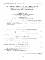
Fig. 1. An example for the frequency dependent linear gainloss function g(ω, z) of equation (4) at z = 0 in a three-channel
system.

existence of steady-state transmission with equal amplitudes for all sequences is retained, while radiation emission
effects are minimized. More specifically, g(ω, z) is equal to
a value gj , required to balance amplitude shifts due to nonlinear gain-loss and Raman crosstalk, inside a frequency
interval of width W centered about the frequency of the
jth-channel solitons at distance z, βj (z), and is equal to
a negative value gL elsewhere2 . Thus, g(ω, z) is given by:
⎧
g if βj (z) − W/2 < ω ≤ βj (z) + W/2
⎪
⎨ j
for 1 ≤ j ≤ N,
g(ω, z) =
⎪
⎩
gL elsewhere,
(4)
where gL < 0. The width W in equation (4) satisfies 1 <
W ≤ Δβ, where Δβ = βj+1 (0) − βj (0) for 1 ≤ j ≤ N − 1.

The values of the gj coefficients are determined by the generalized predator-prey model for collision-induced amplitude dynamics, such that amplitude shifts due to Raman
crosstalk and nonlinear gain-loss are compensated for by
the linear gain-loss. The values of gL and W are determined by carrying out numerical simulations with equations (1), (3), and (4), while looking for the set, which
yields the longest stable propagation distance2 . Figure 1
shows a typical example for the frequency dependent linear gain-loss function g(ω, z) at z = 0 for a three-channel
system with g1 = 0.0195, g2 = 0.0267, g3 = 0.0339,
gL = −0.5, β1 (0) = −15, β2 (0) = 0, β3 (0) = 15, and
W = 10. These parameter values are used in the numerical simulations, whose results are shown in Figure 7 at
the end of Section 4.
The optical pulses in the jth sequence are fundamental solitons of the unperturbed NLS equation with central frequency βj . The envelopes of these solitons are
given by ψsj (t, z) = ηj exp(iχj )sech(xj ), where xj =
ηj (t − yj − 2βj z), χj = αj + βj (t − yj ) + ηj2 − βj2 z,
and ηj , yj , and αj are the soliton amplitude, position,
and phase. Due to the large frequency differences between
2

Note that a similar approach for mitigation of radiative instability was employed in reference [20] for soliton propagation
in the presence of delayed Raman response in the absence of
nonlinear gain-loss.

2.2 A generalized N-dimensional predator-prey model
for amplitude dynamics
The design of waveguide setups for transmission stabilization and switching is based on the derivation of LV
models for dynamics of soliton amplitudes. For this purpose, we consider propagation of N soliton sequences in
a waveguide loop, and assume that the frequency spacing Δβ between the sequences is a large constant, i.e.,
Δβ = |βj+1 (z) − βj (z)|
1 for 1 ≤ j ≤ N − 1. Similar to
references [15,16], we can show that amplitude dynamics
of the N sequences is approximately described by a generalized N -dimensional predator-prey model. The derivation of the predator-prey model is based on the following
assumptions:

(1) The temporal separation T between adjacent solitons
in each sequence satisfies: T
1. In addition, the
amplitudes are equal for all solitons from the same
sequence, but are not necessarily equal for solitons
from different sequences. This setup corresponds, for
example, to phase-shift-keyed soliton transmission.
(2) As T
1, intrasequence interaction is exponentially
small and is neglected.
(3) Delayed Raman response and gain-loss are assumed to
be weak perturbations. As a result, high-order effects
due to radiation emission are neglected, in accordance
with single-collision analysis.
Since the pulse sequences are periodic, the amplitudes of
all solitons in a given sequence undergo the same dynamics. Taking into account collision-induced amplitude shifts
due to broadband delayed Raman response and singlepulse amplitude changes induced by gain and loss, we obtain the following equation for amplitude dynamics of the
jth-sequence solitons (see Refs. [15,16] for similar derivations):
dηj
= ηj gj + F (ηj ) + C
dz

N

(k − j)f (|j − k|)ηk , (5)
k=1

where 1 ≤ j ≤ N , and C = 4 R Δβ/T . The function F (ηj )
on the right hand side of equation (5) is a polynomial in
ηj , whose form is determined by the form of L |ψj |2 .

For L1 and L2 given by equations (2) and (3), we obtain


Eur. Phys. J. D (2017) 71: 30

Page 5 of 18

(1)

(2)

F1 (ηj ) = 4 3 ηj2 /3 − 16 5 ηj4 /15 and F2 (ηj ) = −4 3 ηj2 /3,
respectively. The coefficients f (|j − k|) on the right hand
side of equation (5), which describe the strength of Raman
interaction between jth- and kth-sequence solitons, are
determined by the frequency dependence of the Raman
gain. For the widely used triangular approximation for the
Raman gain curve [1,21], in which the gain is a piecewise
linear function of the frequency, f (|j − k|) = 1 for 1 ≤ j ≤
N and 1 ≤ k ≤ N [15].
In order to demonstrate stable scalable control of soliton propagation, we look for an equilibrium state of the
(eq)
system (5) in the form ηj = η > 0 for 1 ≤ j ≤ N . Such
equilibrium state corresponds to steady-state transmission
with equal amplitudes for all sequences. This requirement
leads to:
N

gj = −F (η) − Cη

(k − j)f (|j − k|).

(6)

k=1

Consequently, equation (5) takes the form
dηj
= ηj F (ηj ) − F (η)
dz
N

(k − j)f (|j − k|)(ηk − η) ,

+C

(7)

k=1

which is a generalized predator-prey model for N
species [35,36]. Notice that (η, . . . , η) and (0, . . . , 0) are
equilibrium states of the model for any positive values of
(1)
(2)
3 , 3 , 5 , η, and C.
We point out that the derivation of an N -dimensional
predator-prey model with a general N value is enabled by
the narrow bandwidth of the waveguide’s nonlinear gainloss. Indeed, due to this property, the gain-loss does not
contribute to amplitude shifts in interchannel collisions,

and therefore, three-pulse interaction can be ignored. This
makes the extension of the predator-prey model from
N = 2 to a general N value straightforward. As a result, extending waveguide setup design from N = 2 to a
general N value for waveguides with broadband delayed
Raman response and narrowband nonlinear gain-loss is
also straightforward. This situation is very different from
the one encountered for waveguides with broadband nonlinear gain-loss. In the latter case, interchannel collisions
are strongly affected by the nonlinear gain-loss, and threepulse interaction gives an important contribution to the
collision-induced amplitude shift [17,33]. Due to the complex nature of three-pulse interaction in generic threesoliton collisions in waveguides with broadband nonlinear
gain or loss (see Ref. [33]), it is very difficult to extend
the LV model for amplitude dynamics from N = 2 to a
generic N value for these waveguides. In the absence of
an N -dimensional LV model, it is unclear how to design
setups for stable transmission stabilization and switching
in N -sequence systems with N > 2. As a result, transmission stabilization and switching in waveguides with broadband nonlinear gain-loss have been so far limited to twosequence systems [17–19].

3 Stability analysis for the predator-prey
model (7)
3.1 Introduction
Transmission stabilization and switching are guided by
stability analysis of the equilibrium states of the predatorprey model (7). In particular, in transmission stabilization, we require that the equilibrium state (η, . . . , η) is
asymptotically stable, so that soliton amplitude values
tend to η with increasing propagation distance for all sequences. Furthermore, transmission switching is based on
bifurcations of the equilibrium state (η, . . . , η). To explain
this, we denote by ηth the value of the decision level, distinguishing between on and off transmission states, and
consider transmission switching of M sequences, for example. In off-on switching of M sequences, the values of
one or more of the physical parameters are changed at the
switching distance zs , such that (η, . . . , η) turns from unstable to asymptotically stable. As a result, before switching, soliton amplitudes tend to values smaller than ηth in
M sequences and to values larger than ηth in N − M sequences, while after the switching, soliton amplitudes in
all N sequences tend to η, where η > ηth . This means

that transmission of M sequences is turned on at z > zs .
On-off switching of M sequences is realized by changing
the physical parameters at z = zs , such that (η, . . . , η)
turns from asymptotically stable to unstable, while another equilibrium state with M components smaller than
ηth is asymptotically stable. Therefore, before switching,
soliton amplitudes in all N sequences tend to η, where
η > ηth , while after the switching, soliton amplitudes
tend to values smaller than ηth in M sequences and to
values larger than ηth in N − M sequences. Thus, transmission of M sequences is turned off at z > zs in this
case. In both transmission stabilization and switching we
require that the equilibrium state at the origin is asymptotically stable. This requirement is necessary in order to
suppress radiative instability due to growth of small amplitude waves [17–19].
The setups of transmission switching that we develop
and study in the current paper are different from the
single-pulse switching setups that are commonly considered in nonlinear optics (see, e.g., Ref. [1] for a description
of the latter setups). We therefore point out the main differences between the two approaches to switching. First, in
the common approach, the amplitude value in the off state
is close to zero. In contrast, in our approach, the amplitude
value in the off state only needs to be smaller than ηth ,
although the possibility to extend the switching to very
small amplitude values does increase switching robustness.
Second, in the common approach, the switching is based
on a single collision or on a small number of collisions, and
as a result, it often requires high-energy pulses for its implementation. In contrast, in our approach, the switching
occurs as a result of the cumulative amplitude shift in a
large number of fast interchannel collisions. Therefore, in
this case pulse energies need not be high. Third and most
important, in the common approach, the switching is carried out on a single pulse or on a few pulses. In contrast,

Page 6 of 18

in our approach, the switching is carried out on all pulses
in the waveguide loop (or within a given waveguide span).
As a result, the switching can be implemented with an
arbitrary number of pulses. Because of this property, we
can refer to transmission switching in our approach as
channel switching. Since channel switching is carried out
for all pulses inside the waveguide loop (or inside a given
waveguide span), it can be much faster than conventional
single-pulse switching. More specifically, channel switching can be faster by a factor of M × K compared with
single-pulse switching, where M is the number of channels,
whose transmission is switched, and K is the number of
pulses per channel in the waveguide loop. For example, in
a 100-channel system with 104 pulses per channel, channel
switching can be faster by a factor of 106 compared with
single-pulse switching.
Our channel switching approach can be used in any
application, in which the same “processing” of all pulses
within the same channel is required, where here processing
can mean amplification, filtering, routing, signal processing, etc. A simple and widely known example for channel switching is provided by transmission recovery, i.e.,
the amplification of a sequence of pulses from small amplitudes values below ηth to a desired final value above
it. However, our channel switching approach can actually
be used in a much more general and sophisticated manner. More specifically, let pj represent the transmission
state of the jth channel, i.e., pj = 0 if the jth channel
is off and pj = 1 if the jth channel is on. Then, the N component vector (p1 , . . . , pj , . . . , pN ), where 1 ≤ j ≤ N ,
represents the transmission state of the entire N -channel
system. One can then use this N -component vector to encode information about the processing to be carried out on
different channels in the next “processing station” in the
transmission line. After this processing has been carried

out, the transmission state of the system can be switched
to a new state, (q1 , . . . , qj , . . . , qN ), which represents the
type of processing to be carried out in the next processing
station. Note that the channel switching approach is especially suitable for phase-shift-keyed transmission. Indeed,
in this case, the phase is used for encoding the information, and therefore, no information is lost by operating
with amplitude values smaller than ηth 3 .
3.2 Stability analysis for transmission stabilization
and off-on switching
Let us obtain the conditions on the values of the physical parameters for transmission stabilization and off-on

Eur. Phys. J. D (2017) 71: 30

switching. As explained above, in this case we require that
both (η, . . . , η) and the origin are asymptotically stable
equilibrium states of the predator-prey model (7).
We first analyze stability of the equilibrium state
(η, . . . , η) in a waveguide with a narrowband GL gain-loss
profile, where F (ηj ) = F1 (ηj ). For this purpose, we show
that
N

[ηj − η + η ln (η/ηj )] ,

VL (ηη ) =

(8)

j=1

where η = (η1 , . . . , ηj , . . . , ηN ), is a Lyapunov function for

equation (7)4 . Indeed, we observe that VL (ηη ) ≥ 0 for any
η with ηj > 0 for 1 ≤ j ≤ N , where equality holds only at
the equilibrium point. Furthermore, the derivative of VL
along trajectories of equation (7) satisfies:
N

dVL /dz = −(16 5/15)

(ηj + η)(ηj − η)2

j=1

×

ηj2

2

+ η − 5κ/4 ,

(9)

(1)

where κ = 3 / 5 and 5 = 0. For asymptotic stability,
we require dVL /dz < 0. This condition is satisfied in a
domain containing (η, . . . , η) if 0 < κ < 8η 2 /5. Thus,
VL (ηη ) is a Lyapunov function for equation (7), and the
equilibrium point (η, . . . , η) is asymptotically stable, if
0 < κ < 8η 2 /5 5 . When 0 < κ ≤ 4η 2 /5, (η, . . . , η) is globally asymptotically stable, since in this case, dVL /dz < 0

for any initial condition with nonzero amplitude values.
When 4η 2 /5 < κ < 8η 2 /5, dVL /dz < 0 for amplitude
1/2
values satisfying ηj > 5κ/4 − η 2
for 1 ≤ j ≤ N .
Thus, in this case the basin of attraction of (η, . . . , η) can
1/2
, ∞ for 1 ≤ j ≤ N .
be estimated by
5κ/4 − η 2
For instability, we require dVL /dz > 0 along trajectories
of (7). This inequality is satisfied in a domain containing
(η, . . . , η) if κ > 8η 2 /5. Therefore, (η, . . . , η) is unstable
for κ > 8η 2 /5 5 .
Consider now the stability properties of the origin
for F (ηj ) = F1 (ηj ). Linear stability analysis shows that
(0, . . . , 0) is asymptotically stable (a stable node) when
gj < 0 for 1 ≤ j ≤ N , i.e., when all pulse sequences propagate in the presence of net linear loss. To slightly simplify
the discussion, we now employ the widely accepted triangular approximation for the Raman gain curve [1,21]. In
this case, f (|j −k|) = 1 for 1 ≤ j ≤ N and 1 ≤ k ≤ N [15],
and therefore the net linear gain-loss coefficients take the
form

3

Channel switching can also be implemented in amplitudekeyed transmission. In this case, one should define a second
threshold level ηth2 , satisfying 0 < ηth2 < ηth . The larger decision level ηth is then used to determine the transmission state
of each channel for channel switching, while the smaller decision level ηth2 is used to determine the state of each time-slot
within a given channel. Thus, in this case, the on and off states
for the jth channel are determined by the conditions ηj > ηth

and ηth2 < ηj < ηth , respectively, where ηj is the common
amplitude value for pulses in occupied time slots in the jth
channel.

gj = −F1 (η) − CN (N + 1)η/2 + CN ηj.
4

(10)

It is possible to show that VL (ηη ) of equation (8) is a Lyapunov function for the predator-prey model (7) even for an
mth-order polynomial L with a negative coefficient for the
mth-order term and properly chosen values for the other polynomial coefficients.
5
Linear stability analysis shows that (η, . . . , η) is a stable
focus when 0 < κ < 8η 2 /5 and an unstable focus when κ >
8η 2 /5.


Eur. Phys. J. D (2017) 71: 30

Page 7 of 18

Since gj is increasing with increasing j, it is sufficient to
require gN < 0. Substituting equation (10) into this inequality, we find that the origin is asymptotically stable,
provided that
κ > 4η 2 /5 + 3CN (N − 1)/(8 5 η).

(11)

The same simple condition is obtained by showing that

2
VL (ηη ) = N
j=1 ηj is a Lyapunov function for equation (7).
Let us discuss the implications of stability analysis for
(η, . . . , η) and the origin for transmission stabilization and
off-on switching. Combining the requirements for asymptotic stability of both (η, . . . , η) and the origin, we expect
to observe stable long-distance propagation, for which soliton amplitudes in all sequences tend to their steady-state
value η, provided the physical parameters satisfy
4η 2 /5 + 3CN (N − 1)/(8 5 η) < κ < 8η 2 /5.

(12)

The same condition is required for realizing stable off-on
transmission switching. Using inequality (12), we find that
the smallest value of 5 , required for transmission stabilization and off-on switching, satisfies the simple condition
5

> 15CN (N − 1)/ 32η 3 .

(13)

As a result, the ratio R / 5 should be a small parameter
in N -sequence transmission with N
1. The independence of the stability condition for (η, . . . , η) on N and R
and the simple scaling properties of the stability condition
for the origin are essential ingredients in enabling robust
scalable transmission stabilization and switching.
Similar stability analysis can be carried out for waveguides with other forms of the nonlinear gain-loss F (ηj )4 .
Consider the central example of a waveguide with narrowband cubic loss, where F (ηj ) = F2 (ηj ). One can show that
in this case VL (ηη ), given by equation (8), is a Lyapunov

function for the predator-prey model (7), and that
dVL /dz = − 4

(2)
3 /3

N

(ηj + η)(ηj − η)2 < 0,

[F (ηj ) = F2 (ηj )] and spans with a GL gain-loss profile [F (ηj ) = F1 (ηj )]. In this case, the global stability of
(η, . . . , η) for spans with linear gain-loss and cubic loss can
be used to bring amplitude values close to η from small
initial amplitude values, while the local stability of the origin for spans with a GL gain-loss profile can be employed
to stabilize the propagation against radiation emission.
3.3 Stability analysis for on-off switching
We now describe stability analysis for on-off switching in
waveguides with a GL gain-loss profile, considering the
general case of switching off of M out of N soliton sequences. As explained in Section 3.1, in switching off of M
sequences, we require that (η, . . . , η) is unstable, the origin is asymptotically stable, and another equilibrium state
with M components smaller than ηth is also asymptotically stable. The requirement for instability of (η, . . . , η)
and asymptotic stability of the origin leads to the following condition on the physical parameter values:
κ > max 8η 2 /5, 4η 2/5 + 3CN (N − 1)/(8 5 η) .

In order to obtain guiding rules for choosing the onoff transmission switching setups, it is useful to consider
first the case of switching off of N − 1 out of N sequences.
Suppose that we switch off the sequences 1 ≤ k ≤ j − 1
and j + 1 ≤ k ≤ N . To realize such switching, we require
that (0, . . . , 0, ηsj , 0, . . . , 0) is a stable equilibrium point
of equation (7). The value of ηsj is determined by the

equation
4
2
ηsj
− 5κηsj
/4 − 15gj /(16 5 ) = 0.

for any trajectory with ηj > 0 for 1 ≤ j ≤ N . Thus,
(η, . . . , η) is globally asymptotically stable, regardless of
(2)
the values of η, R , 3 , and N . However, linear stability analysis shows that the origin is a saddle in this case,
i.e., it is unstable. This instability is related to the fact
that in waveguides with cubic loss, soliton sequences with
(2)
j values satisfying j > (N + 1)/2 − 4 3 η/(3CN ) propagate under net linear gain, and are thus subject to radiative instability. The instability of the origin for uniform
waveguides with cubic loss makes these waveguides unsuitable for long-distance transmission stabilization. On
the other hand, the global stability of (η, . . . , η) and its
independence on the physical parameters, make waveguide spans with narrowband cubic loss very suitable for
realizing robust scalable off-on switching in hybrid waveguides. To demonstrate this, consider a hybrid waveguide
consisting of spans with linear gain-loss and cubic loss

(16)

Since the origin is a stable equilibrium point, transmission
switching of N − 1 sequences can be realized by requiring
that equation (16) has two distinct roots on the positive
half of the ηj -axis (the largest of which corresponds to
ηsj ). This requirement is satisfied, provided6 :

(14)

j=1

(15)

5

> 12|gj |

5κ2 .

(17)

Assuming that g1 < g2 < · · · < gN < 0, we see that
the switching off of the N − 1 low-frequency sequences
1 ≤ j ≤ N − 1 is the least restrictive, since it can be
realized with smaller 5 values. For this reason, we choose
to adopt the switching setup, in which sequences 1 ≤ j ≤
N − 1 are switched off. Employing inequality (17) and the
triangular-approximation-based expression (10) for j =
N , we find that equation (16) has two distinct roots on
the positive half of the ηN -axis, provided that
κ > (8η/5) 5κ/4 − η 2 − 15CN (N − 1)/(32 5 η)

1/2

.
(18)
Therefore, the switching off of sequences 1 ≤ j ≤ N −1 can
be realized when conditions (15) and (18) are satisfied7 .

6

Here we use the fact that the origin is a stable node of
equation (7), so that gj < 0 for 1 ≤ j ≤ N .
7
These conditions should be augmented by the condition for
asymptotic stability of (0, . . . , 0, ηsN ).


Page 8 of 18

Eur. Phys. J. D (2017) 71: 30

We now turn to discuss the general case, where
transmission of M out of N sequences is switched off.
Based on the discussion in the previous paragraph, one
might expect that switching off of M sequences can
be most conveniently realized by turning off transmission of the low-frequency sequences, 1 ≤ j ≤ M . This
expectation is confirmed by numerical solution of the
predator-prey model (7) and the coupled-NLS model (1).
For this reason, we choose to employ switching off of
M sequences, in which transmission in the M lowest frequency channels is turned off. Thus, we require
that (0, . . . , 0, ηs(M+1) , . . . , ηsN ) is an asymptotically stable equilibrium point of equation (7). The values of
ηs(M+1) , . . . , ηsN are determined by the following system
of equations
4
2
ηsj
− 5κηsj
/4 − 15gj /(16 5 )

N

(k − j)f (|j − k|)ηsk = 0, (19)

− 15C/(16 5)

k=M+1

where M + 1 ≤ j ≤ N . Employing the triangular approximation for the Raman gain curve and using equation (10),
we can rewrite the system as:
4
2
−5κηsj
/4−15C/(16 5)
ηsj

N

(k−j)ηsk −η 4 +5κη 2 /4

k=M+1

+ 15CN [(N + 1)/2 − j]η/(16 5 ) = 0. (20)
Stability of (0, . . . , 0, ηs(M+1) , . . . , ηsN ) is determined by
calculating the eigenvalues of the Jacobian matrix J at
this point. The calculation yields Jjk = 0 for 1 ≤ j ≤ M
and j = k,
Jjj = −4

(1) 2

3 η /3

+ 16 5 η 4 /15
N

− C N (N + 1)η/2 −

kηsk
k=M+1

N

ηsk j for 1 ≤ j ≤ M, (21)

+ C Nη −

to check that either JMM < 0 or J11 < 0. To find the
other N −M eigenvalues of the Jacobian matrix, one needs
to calculate the determinant of the (N − M ) × (N − M )
matrix, whose elements are Jjk , where M + 1 ≤ j, k ≤ N .
The latter calculation can also be significantly simplified
by noting that for M + 1 ≤ j ≤ N , the diagonal elements are of order 5 , while the off-diagonal elements are
of order N R at most. Thus, the leading term in the ex−M
pression for the determinant is of order N
. The next
5
term in the expansion is the sum of N − M terms, each
−M−2
of which is of order N 2 2R N
at most. Therefore, the

5
next term in the expansion of the determinant is of or−M−2
der (N − M )N 2 2R N
at most. Comparing the first
5
and second terms, we see that the correction term can be
neglected, provided that 5
N 3/2 R . We observe that
the last condition is automatically satisfied by our on-off
transmission switching setup for N
1, since stability
of the origin requires 5 > N 2 R
N 3/2 R (see inequality (15)). It follows that the other N − M eigenvalues of
the Jacobian matrix are well approximated by the diagonal elements Jjj for M + 1 ≤ j ≤ N . Therefore, for
N
1, stability analysis of (0, . . . , 0, ηs(M+1) , . . . , ηsN )
only requires the calculation of N − M + 1 diagonal elements of the Jacobian matrix.
We point out that the preference for the turning off of
transmission of low-frequency sequences in on-off switching is a consequence of the nature of the Raman-induced
energy exchange in soliton collisions. Indeed, Raman
crosstalk leads to energy transfer from high-frequency
solitons to low-frequency ones [25,34,37–41]. To compensate for this energy loss or gain, high-frequency sequences
should be overamplified while low-frequency sequences
should be underamplified compared to mid-frequency sequences [15,20]. As a result, the magnitude of the net linear loss is largest for the low-frequency sequences, and
therefore, on-off switching is easiest to realize for these sequences. It follows that the presence of broadband delayed
Raman response introduces a preference for turning off the
transmission of the low-frequency sequences, and by this,
enables systematic scalable on-off switching in N -sequence
systems.

k=M+1

Jjk = C(k − j)ηsj for M + 1 ≤ j ≤ N and j = k,
(22)

4 Numerical simulations
with the coupled-NLS model

and
Jjj = gj + 4

(1) 2
3 ηsj

4
− 16 5 ηsj
/3

N

+C

(k − j)ηsk for M + 1 ≤ j ≤ N.

(23)

k=M+1

Note that the Raman triangular approximation was used
to slightly simplify the form of equations (21)–(23). Since

Jjk = 0 for 1 ≤ j ≤ M and j = k, the first M eigenvalues
of the Jacobian matrix are λj = Jjj , where the Jjj coefficients are given by equation (21). Furthermore, since Jjj is
either monotonically increasing or monotonically decreasing with increasing j, to establish stability, it is sufficient

The predator-prey model (7) is based on several simplifying assumptions, which might break down with increasing number of channels or at large propagation distances. In particular, equation (7) neglects the effects of
pulse distortion, radiation emission, and intrasequence interaction that are incorporated in the full coupled-NLS
model (1). These effects can lead to transmission destabilization and to the breakdown of the predator-prey
model description [16–20]. In addition, during transmission switching, soliton amplitudes can become small, and
as a result, the magnitude of the linear gain-loss term
in equation (1) might become comparable to the magnitude of the Kerr nonlinearity terms. This can in turn lead


Eur. Phys. J. D (2017) 71: 30

to the breakdown of the perturbation theory, which is the
basis for the derivation of the predator-prey model. It is
therefore essential to test the validity of the predator-prey
model’s predictions by carrying out numerical simulations
with the full coupled-NLS model (1).
The coupled-NLS system (1) is numerically integrated
using the split-step method with periodic boundary conditions [1]. Due to the usage of periodic boundary conditions, the simulations describe pulse propagation in a
closed waveguide loop. The initial condition for the simulations consists of N periodic sequences of 2K solitons
with amplitudes ηj (0), frequencies βj (0), and zero phases:
K−1

ψj (t, 0) =
k=−K

ηj (0) exp{iβj (0)[t − (k + 1/2)T − δj ]}
,

cosh{ηj (0)[t − (k + 1/2)T − δj ]}

(24)
where the frequency differences satisfy Δβ = βj+1 (0) −
βj (0)
1, for 1 ≤ j ≤ N − 1. The coefficients δj represent
the initial position shift of the jth sequence solitons relative to pulses located at (k+1/2)T for −K ≤ k ≤ K−1. To
maximize propagation distance in the presence of delayed
Raman response, we use δj = (j − 1)T /N for 1 ≤ j ≤ N .
As a concrete example, we present the results of numerical
simulations for the following set of physical parameters:
T = 15, Δβ = 15, and K = 1. In addition, we employ
the triangular approximation for the Raman gain curve,
so that the coefficients f (|j − k|) satisfy f (|j − k|) = 1 for
1 ≤ j, k ≤ N [15,20]. We emphasize, however, that similar results are obtained with other choices of the physical
parameter values, satisfying the stability conditions discussed in Section 3.
We first describe numerical simulations for transmission stabilization in waveguides with broadband delayed
Raman response and a narrowband GL gain-loss profile
L |ψj |2 = L1 |ψj |2 for N = 2, N = 3, and N = 4
sequences. We choose η = 1 so that the desired steady
state of the system is (1, . . . , 1). The Raman coefficient is
R = 0.0006, while the quintic loss coefficient is 5 = 0.1
for N = 2, 5 = 0.15 for N = 3, and 5 = 0.25 for
N = 4. In addition, we choose κ = 1.2 and initial ampli1/2
tudes satisfying ηj (0) > 5κ/4 − η 2
for 1 ≤ j ≤ N , so
that the initial amplitudes belong to the basin of attraction of (1, . . . , 1). The numerical simulations with equations (1) and (2) are carried out up to the final distances
zf1 = 36 110, zf2 = 21 320, and zf3 = 5350, for N = 2,
N = 3, and N = 4, respectively. At these distances,
the onset of transmission destabilization due to radiation

emission and pulse distortion is observed. The z dependence of soliton amplitudes obtained by the simulations
is shown in Figures 2a, 2c, and 2e together with the prediction of the predator-prey model (7). Figures 2b, 2d,
and 2f show the amplitude dynamics at short distances.
Figures 3a, 3c, and 3e show the pulse patterns |ψj (t, z)| at
a distance z = zr before the onset of transmission instability, where zr1 = 36 000 for N = 2, zr2 = 21 270 for N = 3,
and zr3 = 5300 for N = 4. Figures 3b, 3d, and 3f show
the pulse patterns |ψj (t, z)| at z = zf , i.e., at the onset
of transmission instability. As seen in Figure 2, the soli-

Page 9 of 18

ton amplitudes tend to the equilibrium value η = 1 with
increasing distance for N = 2, 3, and 4, i.e., the transmission is stable up to the distance z = zr in all three cases.
The approach to the equilibrium state takes place along
distances that are much shorter compared with the distances along which stable transmission is observed. Furthermore, the agreement between the predictions of the
predator-prey model and the coupled-NLS simulations is
excellent for 0 ≤ z ≤ zr . Additionally, as seen in Figures 3a, 3c, and 3e, the solitons retain their shape at z = zr
despite the large number of intersequence collisions. The
distances zr , along which stable propagation is observed,
are significantly larger compared with those observed in
other multisequence nonlinear waveguide systems. For example, the value zr1 = 36 000 for N = 2 is larger by a factor of 200 compared with the value obtained in waveguides
with linear gain and broadband cubic loss [16]. Moreover,
the stable propagation distances observed in the current
work for N = 2, N = 3, and N = 4 are larger by factors of
37.9, 34.3, and 10.6 compared with the distances obtained
in single-waveguide transmission in the presence of delayed
Raman response and in the absence of nonlinear gainloss [20]. The latter increase in the stable transmission
distances is quite remarkable, considering the fact that in
reference [20], intrasequence frequency-dependent linear
gain-loss was employed to further stabilize the transmission, whereas in the current work, the gain-loss experienced by each sequence is uniform. We also point out that

the results of our numerical simulations provide the first
example for stable long-distance propagation of N soliton
sequences with N > 2 in systems described by coupled
GL models.
We note that at the onset of transmission instability,
the pulse patterns become distorted, where the distortion
appears as fast oscillations of |ψj (t, z)| that are most pronounced at the solitons’ tails (see Figs. 3b, 3d, and 3f).
The degree of pulse distortion is different for different
pulse sequences. Indeed, for N = 2, the j = 1 sequence
is significantly distorted at z = zf1 , while no significant
distortion is observed for the j = 2 sequence. For N = 3,
the j = 1 sequence is significantly distorted, the j = 3
sequence is slightly distorted, while the j = 2 sequence
is still not distorted at z = zf2 . For N = 4, the j = 1
and j = 4 sequences are both significantly distorted at
z = zf3 , while no significant distortion is observed for the
j = 2 and j = 3 sequences at this distance.
The distortion of the pulse patterns and the associated transmission destabilization can be explained by
examination of the Fourier transforms of the pulse patterns ψˆj (ω, z) . Figure 4 shows the Fourier transforms
ψˆj (ω, z) at z = zr (before the onset of transmission instability) and at z = zf (at the onset of transmission instability). Figure 5 shows magnified versions of the graphs
in Figure 4 for small ψˆj (ω, z) values. It is seen that the
Fourier transforms of some of the pulse sequences develop
pronounced radiative sidebands at z = zf . Furthermore,
the frequencies at which the radiative sidebands attain
their maxima are related to the central frequencies βj (z)


Page 10 of 18

Eur. Phys. J. D (2017) 71: 30

(a)

1.3
1.2

1.2

1.1

1.1

ηj

η

j 1

1

0.9

0.9

0.8

0.8

0.7
0

5000 10000 15000 20000 25000 30000 35000

z

(c)

1.3

1.2

1.1

1.1

j 1

η 1
j

0.9

0.9

0.8

0.8
5000

10000

z

15000

20000

(e)

1.3

0.7
0

1.2

1.1

1.1

ηj

1

0.9

0.8

0.8
1000

2000

z 3000

4000

5000

z

60

80

100

30

40

50

30

40

50

(d)

10

20

z
(f)

1

0.9

0.7
0

40

1.3

1.2

j

20

1.3

η

η

0.7
0

1.2

0.7
0

(b)

1.3

0.7
0

10

20

z

Fig. 2. The z dependence of soliton amplitudes ηj during transmission stabilization in waveguides with broadband delayed
Raman response and narrowband GL gain-loss for two-sequence ((a) and (b)), three-sequence ((c) and (d)), and four-sequence
((e) and (f)) transmission. Graphs (b), (d), and (f) show magnified versions of the ηj (z) curves in graphs (a), (c), and (e)
at short distances. The red circles, green squares, blue up-pointing triangles, and magenta down-pointing triangles represent
η1 (z), η2 (z), η3 (z), and η4 (z), obtained by numerical simulations with equations (1) and (2). The solid brown, dashed gray,
dashed-dotted black, and solid-starred orange curves correspond to η1 (z), η2 (z), η3 (z), and η4 (z), obtained by the predator-prey
model (7).

of the soliton sequences or to the frequency spacing Δβ.

The latter observation indicates that the processes leading to radiative sideband generation are resonant in nature
(see also Refs. [20,42]).
Consider first the Fourier transforms of the pulse patterns for N = 2. As seen in Figures 4b and 5b, in this
case the j = 1 sequence develops radiative sidebands at
(11)
(12)
frequencies ωs
= 17.18 and ωs
= 34.76 at z = zf1 .
In contrast, no significant sidebands are observed for the
j = 2 sequence at this distance. These findings explain
the significant pulse pattern distortion of the j = 1 sequence and the absence of pulse pattern distortion for
the j = 2 sequence at z = zf1 . In addition, the radiative sideband frequencies satisfy the simple relations:
(11)
(12)
(11)
ωs − β2 (zr1 ) ∼ 29.3 ∼ 2Δβ and ωs
∼ 2ωs . For

N = 3, the j = 1 sequence develops significant sidebands
(11)
(12)
= 0.0 and ωs
= 44.4, the j = 3
at frequencies ωs
(31)
sequence develops a weak sideband at frequency ωs =
−31.42, and the j = 2 sequence does not have any significant sidebands at z = zf2 (see Figs. 4d and 5d). These
results coincide with the significant pulse pattern distortion of the j = 1 sequence, the weak pulse pattern distortion of the j = 3 sequence, and the absence of pulse
pattern distortion for the j = 2 sequence at z = zf2 . Additionally, the sideband frequencies satisfy the simple rela(11)

(12)
(31)
tions: ωs ∼ β3 (zr2 ), ωs ∼ 3Δβ, and ωs ∼ β1 (zr2 ).
For N = 4, the j = 1 and j = 4 sequences develop significant sidebands, while no significant sidebands are observed for the j = 2 and j = 3 sequences at z = zf3
(see Figs. 4f and 5f). These findings explain the significant


Eur. Phys. J. D (2017) 71: 30

Page 11 of 18
(b)

(a)
1

|ψj (t, zf1 = 36110)|

|ψj (t, zr1 = 36000)|

1
0.8
0.6
0.4
0.2
0
−15

−10

−5

0

t

5

10

0.8
0.6
0.4
0.2
0
−15

15

−10

−5

|ψj (t, zf2 = 21320)|

|ψj (t, zr2 = 21270)|

1
0.8
0.6
0.4

0.2
−10

−5

0

t

10

15

5

10

5

10

15

5

10

15

0.8

0.6
0.4
0.2
0
−15

15

−10

−5

(e)

0

t

(f)
1

|ψj (t, zf3 = 5350)|

|ψj (t, zr3 = 5300)|

5

1

1

0.8
0.6
0.4
0.2
0
−15

t

(d)

(c)

0
−15

0

−10

−5

0

t

5

10

15

0.8
0.6
0.4
0.2
0
−15

−10

−5

0

t

Fig. 3. The pulse patterns |ψj (t, z)| near the onset of transmission instability for the two-sequence ((a) and (b)), three-sequence
((c) and (d)), and four-sequence ((e) and (f)) transmission setups considered in Figure 2. Graphs (a), (c), and (e) show |ψj (t, z)|
before the onset of instability, while graphs (b), (d), and (f) show |ψj (t, z)| at the onset of instability. The solid red curve,
dashed-dotted green curve, blue crosses, and dashed magenta curve represent |ψj (t, z)| with j = 1, 2, 3, 4, obtained by numerical
solution of equations (1) and (2). The propagation distances are z = zr1 = 36 000 (a), z = zf1 = 36 110 (b), z = zr2 = 21 270
(c), z = zf2 = 21 320 (d), z = zr3 = 5300 (e), and z = zf3 = 5350 (f).

pulse pattern distortion of the j = 1 and j = 4 sequences
and the absence of significant pulse pattern distortion for
the j = 2 and j = 3 sequences at z = zf3 . The sideband
frequencies of the j = 1 sequence satisfy the relations:
(11)
(12)

(11)
ωs = 17.17 ∼ β3 (zr3 ), and ωs = 34.77 ∼ 2ωs . Note
(11)
(12)
that the values of ωs
and ωs
for N = 4 are very
close to the values found for N = 2. Finally, the sideband
frequencies of the j = 4 sequence satisfy the relations:
(41)
(42)
(11)
ωs = −27.65 ∼ β1 (zr3 ), and ωs = 34.35 ∼ 2ωs .
We now turn to describe numerical simulations for a
single transmission switching event in waveguides with
broadband delayed Raman response and a narrowband GL
gain-loss profile. As described in Section 3, on-off switching of M out of N pulse sequences at a distance z = zs
is realized by changing the value of one or more of the

physical parameters, such that the steady state (η, . . . , η)
turns from asymptotically stable to unstable, while another steady state at (0, . . . , 0, ηs(M+1) , . . . , ηsN ) is asymptotically stable. We denote the on-off switching setups by
A1-A2, where A1 and A2 denote the sets of physical parameters used at 0 ≤ z < zs and z ≥ zs , respectively.
Off-on switching of M out of N soliton sequences at
z = zs is realized by changing the physical parameter values such that (η, . . . , η) turns from unstable to asymptotically stable. As explained in Section 3, to achieve stable long-distance transmission after the switching, one
needs to require that the origin is an asymptotically stable steady state as well. Under this requirement, κ must
satisfy inequality (12), and as a result, the basin of attraction of (η, . . . , η) is limited to

5κ/4 − η 2

1/2

,∞


Page 12 of 18

Eur. Phys. J. D (2017) 71: 30
(b)

(a)

|ψˆj (ω, zf1 = 36110)|

|ψˆj (ω, zr1 = 36000)|

2.5
2

1.5
1

0.5
0
−40 −30 −20 −10

ω 10

0

20

30

40

2.5
2
1.5
1
0.5
0
−40 −30 −20 −10

50

0

2

30

20

30

20

30

40

50

1.5
1
0.5
−40 −30 −20 −10

0

ω 10

20

30

40

2
1.5
1
0.5
0

50

−40 −30 −20 −10

0

(e)

40

50

(f)

|ψˆj (ω, zf3 = 5350)|

2
1.5
1
0.5
0
−40 −30 −20 −10

ω 10

2.5

2.5

|ψˆj (ω, zr3 = 5300)|

20

2.5

2.5

0

ω 10
(d)

|ψˆj (ω, zf2 = 21320)|

|ψˆj (ω, zr2 = 21270)|

(c)

0

ω 10

20

30

40

50

2
1.5
1
0.5
0
−40 −30 −20 −10

0

ω 10

40

50

Fig. 4. The Fourier transforms of the pulse patterns ψˆj (ω, z) near the onset of transmission instability for the two-sequence
((a) and (b)), three-sequence ((c) and (d)), and four-sequence ((e) and (f)) transmission setups considered in Figures 2 and 3.
Graphs (a), (c), and (e) show ψˆj (ω, z) before the onset of instability, while graphs (b), (d), and (f) show ψˆj (ω, z) at the onset
of instability. The red circles, green squares, blue up-pointing triangles, and magenta down-pointing triangles represent ψˆj (ω, z)
with j = 1, 2, 3, 4, obtained by numerical solution of equations (1) and (2). The propagation distances are z = zr1 = 36 000 (a),
z = zf1 = 36 110 (b), z = zr2 = 21 270 (c), z = zf2 = 21 320 (d), z = zr3 = 5300 (e), and z = zf3 = 5350 (f).

for 1 ≤ j ≤ N . This leads to limitations on the turning
on of the M sequences, especially for M ≥ 2 and N ≥ 3.
To overcome this difficulty, we consider a hybrid waveguide consisting of a span with a GL gain-loss profile, a
span with linear gain-loss and cubic loss, and a second
span with a GL gain-loss profile. The introduction of the
intermediate waveguide span with linear gain-loss and cubic loss enables the turning on of the M sequences from
low amplitude values due to the global stability of the
steady state (η, . . . , η) for the corresponding predator-prey
model. However, due to the presence of linear gain and the
instability of the origin for the same predator-prey model,
propagation in the waveguide span with linear gain-loss
and cubic loss is unstable against emission of small amplitude waves. For this reason, we introduce the frequency

dependent linear gain-loss g(ω, z) of equation (4) when

simulating propagation in the second span. More importantly, propagation in the second span with a GL gain-loss
profile leads to mitigation of radiative instability due to
the presence of linear loss in all channels for this waveguide span. This enables stable long-distance propagation
of the N soliton sequences after the switching. We denote
the off-on switching setups by A2-B-A1, where A2, B, and
A1 denote the sets of physical parameters used in the first,
second, and third spans of the hybrid waveguide. The first
span is located at [0, zs1 ), the second at [zs1 , zs2 ), and the
third at [zs2 , zf ], where zf is the final propagation distance. Thus, off-on switching of the M soliton sequences
occurs at z ≥ zs1 , while final transmission stabilization
takes place at z ≥ zs2 .


Eur. Phys. J. D (2017) 71: 30
−6

(a)

|ψˆj (ω, zf1 = 36110)|

2.5
2
1.5
1
0.5
0
−50 −40 −30 −20 −10
−3

|ψˆj (ω, zr2 = 21270)|

6 x 10

0

ω

10

20

30

40

0
−40 −30 −20 −10

0

2
1
0

ω

10

20

30

40

30

20

30

40

50

0.1

0

50

−40 −30 −20 −10

|ψˆj (ω, zf3 = 5350)|

|ψˆj (ω, zr3 = 5300)|

0.6

0.02

0.01

ω

20

0.2

(e)

0

ω 10
(d)

3

0
−40 −30 −20 −10

0.1

(c)

4

0.03

0.2

50

5

0
−50 −40 −30 −20 −10

(b)

0.3

|ψˆj (ω, zf2 = 21320)|

|ψˆj (ω, zr1 = 36000)|

3 x 10

Page 13 of 18

10

20

30

40

ω 10

0

40

50

(f)

0.5
0.4
0.3
0.2
0.1
0
−40 −30 −20 −10

0

ω

10

20

30

40

Fig. 5. Magnified versions of the graphs in Figure 4 for small |ψˆj (ω, z)| values. The symbols and distances are the same as in
Figure 4.

We present here the results of numerical simulations
for on-off and off-on switching of two and three soliton
sequences in four-sequence transmission. As discussed in
the preceding paragraphs, on-off switching setups are denoted by A1-A2 and off-on switching setups are denoted
by A2-B-A1. The following values of the physical parameters are used. The Raman coefficient is R = 0.0006, which
is the same value used in transmission stabilization. The
other parameter values used in setup A1 in both on-off
and off-on switching are 5 = 0.1, κ = 1.2, and η = 1.
The parameter values used in setup A2 in on-off switching are 5 = 0.04, κ = 1.8, and η = 1.05 for M = 2
and 5 = 0.04, κ = 2, and η = 1.1 for M = 3. The
on-off switching distance is zs = 250 for both M = 2
and M = 3. The parameter values used in setup A2 in
off-on switching are 5 = 0.032, κ = 2.2, and η = 1.1
for M = 2 and 5 = 0.02, κ = 2.8, and η = 1.3 for
M = 3. The parameter values used in off-on switching in
(2)
setup B are 3 = 0.02 and η = 1 for both M = 2 and
M = 3. To suppress radiative instability during propa-

gation in waveguide spans with linear gain-loss and cubic
loss (setup B), the frequency dependent linear gain-loss
g(ω, z) of equation (4) with W = 10 and gL = −0.5 is
employed. The switching and final stabilization distances
in off-on transmission switching are zs1 = 30 and zs2 = 80
for M = 2, and zs1 = 30 and zs2 = 90 for M = 3. We point
out that similar results were obtained with other choices
of the physical parameter values, satisfying the stability
conditions discussed in Section 3.
The results of numerical simulations with equations (1)
and (2) for on-off switching of two and three soliton sequences in four-sequence transmission in setup A1-A2 are

shown in Figures 6a and 6b. The results of simulations
with equations (1)–(4) for off-on switching of two and
three sequences in four-sequence transmission in setup
A2-B-A1 are shown in Figures 6c and 6d. A comparison with the predictions of the predator-prey model (7) is
also presented. The agreement between the coupled-NLS
simulations and the LV model’s predictions is excellent
in all four cases. More specifically, in on-off transmission


Page 14 of 18

Eur. Phys. J. D (2017) 71: 30
(a)

1.4
1.2

1.2

1

1

0.8

ηj

η

0.8

j

0.6

0.6

0.4

0.4

0.2

0.2

0
0

100

200

z

(b)

1.4

300

400

0
0

500

100

200

(c)

300

400

500

600

800

1000

(d)

1.6

1.4

1.4

1.2

1.2

1

η

j 1

ηj

0.8
0.6

0.8
0.6

0.4

0.4

0.2

0.2

0

0

z

200

400

z

600

800

1000

0
0

200

400

z

Fig. 6. The z dependence of soliton amplitudes ηj during single transmission switching events in four-sequence transmission
in waveguides with broadband delayed Raman response and narrowband nonlinear gain-loss. (a) and (b) show on-off switching
of two and three soliton sequences in waveguides with a GL gain-loss profile in setup A1-A2, while (c) and (d) show off-on
switching of two and three sequences in hybrid waveguides in setup A2-B-A1. The red circles, green squares, blue up-pointing
triangles, and magenta down-pointing triangles represent η1 (z), η2 (z), η3 (z), and η4 (z), obtained by numerical simulations with

equations (1) and (2) in (a) and (b), and with equations (1)–(4) in (c) and (d). The solid brown, dashed gray, dashed-dotted
black, and solid-starred orange curves correspond to η1 (z), η2 (z), η3 (z), and η4 (z), obtained by the predator-prey model (7).

switching of M sequences with M = 2 and M = 3, the
amplitudes of the solitons in the M lowest frequency channels tend to zero, while the amplitudes of the solitons in
the N −M high frequency channels tend to new values ηsj ,
where M + 1 ≤ j ≤ N . The values of the new amplitudes
are ηs3 = 1.2499 and ηs4 = 1.2878 in on-off switching of
two sequences, and ηs4 = 1.3640 in on-off switching of
three sequences. As can be seen from Figures 6a and 6b,
these values are in excellent agreement with the predictions of the predator-prey model (7). In off-on switching
of M soliton sequences, the amplitudes of the solitons in
the M low frequency channels tend to zero for z < zs1 ,
while the amplitudes of the solitons in the N − M high
frequency channels increase with z for z < zs1 . After the
switching, i.e., for distances z ≥ zs1 , the amplitudes of the
solitons in the M low frequency channels increase to the
steady-state value of 1, while the amplitudes of the solitons in the N − M high frequency channels decrease and
tend to 1, in full agreement with the predator-prey model’s
predictions. Note that very good agreement between the
coupled-NLS and predator-prey models is observed even
when some of the soliton amplitudes are small, i.e., even
outside of the perturbative regime, where the predatorprey model is expected to hold. The results of the simulations presented in Figure 6 and similar results obtained
with other sets of the physical parameters demonstrate

that it is indeed possible to realize stable scalable on-off
and off-on transmission switching in the waveguide setups
considered in the current study. Furthermore, the simulations confirm that design of the switching setups can be
guided by stability and bifurcation analysis for the steady
states of the predator-prey model (7). We point out that

the off-on switching setups can also be employed in broadband transmission recovery, that is, in the simultaneous
amplification of multiple soliton sequences, which experienced significant energy decay, to a desired steady-state
amplitude value.
As discussed in Section 3, an important application
of the switching setups considered in our paper is for realizing efficient signal processing in multichannel transmission. In such application, the amplitude values ηj are
used to encode information about the type of signal processing to be carried out in the next processing station. As a result, the pulse sequences typically undergo
multiple switching events and it is important to show
that this can be realized in a stable manner. We therefore turn to discuss the results of numerical simulations
with the coupled-NLS model (1) for multiple switching
events. As a specific example, we consider multiple switching in a three-channel system in the hybrid waveguide
setup A1-(A2-B-A1)-. . . -(A2-B-A1), where (A2-B-A1) repeats six times. Thus, in this case the soliton sequences


Eur. Phys. J. D (2017) 71: 30

5 Discussion
Let us discuss the reasons for the robustness and scalability of transmission stabilization and switching in

(a)

1.6
1.4

ηj

1.2
1
0.8
0.6
0.4

0.2
0
0

1000

2000

z

3000

4000

5000

(b)
1

|ψj (t, zf = 5000)|

first experience transmission stabilization in waveguide
setup A1, and then undergo six successive off-on switching
events in waveguide setup A2-B-A1. The parameter values
are chosen such that during on switching, amplitude values in all sequences tend to 1, while during off switching,
transmission of a single sequence (the lowest-frequency sequence j = 1) is turned off. We emphasize, however, that
similar results are obtained with other numbers of channels and in other switching scenarios. For the example presented here, during on switching stabilization in waveguide
setup A1, R = 0.0006, 5 = 0.15, κ = 1.2, and η = 1 are
used, while during off switching in waveguide setup A2,
R = 0.0024, 5 = 0.024, κ = 2.2, and η = 1.15 are used.

Note that the higher value of R in waveguide setup A2 is
required for realizing a faster on-off transmission switching, that is, for decreasing the distance along which the
off switching takes place. Additionally, during on switch(2)
ing in waveguide setup B, R = 0.0006, 3 = 0.02, and
η = 1 are chosen. To suppress radiative instability during propagation in waveguide spans with linear gain-loss
and cubic loss (setup B), the frequency dependent linear gain-loss g(ω, z) of equation (4) with W = 10 and
gL = −0.5 is employed. In the simulations, transmission
of the j = 1 sequence is turned off in setup A2 at distances z3m+1 = 700(m + 1) for 0 ≤ m ≤ 5. Transmission of sequence j = 1 is turned on in waveguide setup
B at z3m+2 = 50 + 700(m + 1) for 0 ≤ m ≤ 5, and
transmission stabilization in setup A1 starts at z0 = 0
and at z3m = 100 + 700m for 1 ≤ m ≤ 6. The final
propagation distance is zf = 5000. Thus, the waveguide
spans are [0, 700), [700, 750), [750, 800), [800, 1400), . . . ,
[4200, 4250), [4250, 4300), and [4300, 5000].
The results of numerical simulations with equations (1)–(4) for multiple transmission switching events
are shown in Figure 7 along with the predictions of
the predator-prey model (7). The agreement between the
coupled-NLS simulations and the predator-prey model’s
predictions is excellent throughout the propagation. Furthermore, as seen in Figure 7b, no pulse distortion is observed at the final propagation distance zf . Note that the
minimal values of η1 (z), which are attained prior to the
start of the on switch, are η1 (z3m+2 ) = 0.33. As a result,
the value of the decision level ηth for distinguishing between on and off transmission states can be set as low
as ηth = 0.35, which is significantly lower than the value
ηth = 0.65 obtained in reference [18] for transmission in
a two-channel waveguide system with a broadband GL
gain-loss profile. The results presented in Figure 7 along
with results of numerical simulations with other sets of the
physical parameter values demonstrate that stable multiple transmission switching events can indeed be realized
over a wide range of amplitude values, using waveguides
with broadband delayed Raman response and narrowband

nonlinear gain-loss.

Page 15 of 18

0.8
0.6
0.4
0.2
0
−15

−10

−5

0

t

5

10

15

Fig. 7. (a) The z dependence of soliton amplitudes ηj in multiple transmission switching with three sequences (N = 3) in
hybrid waveguide setup A1-(A2-B-A1)-. . . -(A2-B-A1), where
(A2-B-A1) repeats six times. In this case, the soliton sequences
undergo transmission stabilization followed by six successive
off-on switching events. The red circles, green squares, and

blue up-pointing triangles represent η1 (z), η2 (z), and η3 (z),
obtained by numerical simulations with equations (1)–(4). The
solid brown, dashed gray, and dashed-dotted black curves correspond to η1 (z), η2 (z), and η3 (z), obtained by the predatorprey model (7). (b) The pulse patterns |ψj (t, z)| at the final
distance z = zf = 5000, as obtained by numerical solution
of equations (1)–(4). The solid red curve, dashed-dotted green
curve, and blue crosses represent |ψj (t, z)| with j = 1, 2, 3.

waveguides with broadband delayed Raman response and
narrowband nonlinear gain-loss. The scalability and robustness of transmission control can be attributed to the
following properties of these waveguides:
(1) The asymptotic stability of the steady state (η, . . . , η)
for waveguides with a GL gain-loss profile, which is
independent of N and R , is key to realizing scalable
transmission stabilization and switching.
(2) The presence of net linear loss in all frequency channels for waveguides with a GL gain-loss profile leads
to mitigation of radiative instability.
(3) Due to the narrow bandwidth of the nonlinear gainloss, three-pulse interaction does not contribute to
collision-induced amplitude shifts. As a result, the extension of the predator-prey model from N = 2 to a
general N value is straightforward. This also makes
the extension of waveguide setup design from N = 2


Page 16 of 18

to a general N value straightforward. In contrast,
in waveguides with broadband nonlinear gain-loss,
three-pulse interaction gives an important contribution to collision-induced amplitude shifts [17,33]. Due
to the complex nature of three-pulse interaction in
generic three-soliton collisions in waveguides with
broadband nonlinear gain or loss (see Ref. [33]), it

is very difficult to extend the LV model for amplitude dynamics from N = 2 to a generic N value in
these waveguides. In the absence of an N -dimensional
LV model, it is unclear how to design setups for stable transmission stabilization and switching in N sequence waveguide systems with broadband nonlinear gain-loss. As a result, transmission stabilization
and switching in waveguides with broadband nonlinear gain-loss have been so far limited to two-sequence
systems [17–19].
(4) The Raman-induced energy transfer in soliton collisions from high-frequency solitons to low-frequency
solitons is an important ingredient in the realization
of scalable on-off switching. Indeed, to compensate for
the Raman-induced energy loss or gain in the collisions, high-frequency sequences should be overamplified while low-frequency sequences should be underamplified compared to mid-frequency sequences.
As a result, the magnitude of the net linear loss is
largest for the low-frequency sequences, and therefore, on-off switching is easiest to realize for these
sequences. Thus, the presence of broadband delayed
Raman response introduces a preference for turning
off the transmission of the low-frequency sequences,
and by this enables systematic scalable on-off switching.
(5) The global asymptotic stability of the steady state
(η, . . . , η) for waveguide spans with linear gain-loss
and cubic loss, which is independent of all physical
parameters, is important for realizing robust scalable
off-on switching in hybrid waveguides.
These five waveguide properties are explained by stability and bifurcation analysis for the steady states of the
generalized N -dimensional predator-prey model for amplitude dynamics. Thus, the analysis of the predator-prey
model is essential to the design of waveguide setups leading to stable scalable control of soliton-based multichannel
transmission.
Note that waveguide setups with narrowband cubic
gain and quinitc loss or with narrowband cubic loss can
be realized by employing fast saturable absorbers with a
bandwidth ΔνGL satisfying: ν0
ΔνGL
Δν. That

is, in these waveguide systems, the bandwidth of the saturable absorber is larger than the spectral width of the
optical pulses but smaller than the frequency spacing between adjacent frequency channels. Waveguide systems
containing a fast saturable absorber with a finite spectral
width, which is much larger than the spectral width of the
optical pulses, have been studied extensively in the context
of mode-locked lasers; see, for example, references [43–45]
and references therein.

Eur. Phys. J. D (2017) 71: 30

6 Conclusions
We developed a method for achieving stable scalable control of propagation of multiple soliton sequences in broadband optical waveguide systems. The method is based
on employing nonlinear waveguides with broadband delayed Raman response, linear gain-loss, and narrowband
nonlinear gain-loss. We showed that the combination of
Raman-induced amplitude shifts in interchannel collisions
and single-pulse amplitude shifts due to linear and nonlinear gain-loss with properly chosen physical parameter
values can be used to realize robust scalable transmission stabilization and switching. For this purpose, we first
showed that the dynamics of soliton amplitudes in an
N -sequence transmission system can be described by a
generalized N -dimensional predator-prey model. We then
carried out stability and bifurcation analysis for the steady
states of the predator-prey model for two central cases of
the gain-loss: (1) a GL gain-loss profile; (2) linear gain-loss
and cubic loss. The stability and bifurcation analysis was
then used to develop waveguide setups that lead to robust transmission stabilization as well as on-off and off-on
switching of M out of N soliton sequences.
For waveguides with a GL gain-loss profile, we obtained the Lyapunov function VL (ηη ) for the predator-prey
model and used it to derive simple conditions for asymptotic stability and instability of the steady state with equal
amplitudes for all sequences (η, . . . , η). These conditions
are independent of the number of channels N and the

value of the Raman coefficient R , which is essential for
the realization of scalable transmission stabilization and
switching. We also found that the steady state at the origin is asymptotically stable, provided all the linear gainloss coefficients are negative. Combining the requirements
for asymptotic stability of both (η, . . . , η) and the origin,
we showed that the smallest value of the quintic loss coefficient 5 required for robust transmission stabilization
and off-on switching for N
1 scales as 5 ∼ N 2 R .
The realization of on-off switching requires stability analysis of steady states, for which M components are equal
to zero. We first gave a simple argument, showing that
switching off of M sequences is most conveniently realized
by turning off the transmission of the low-frequency sequences 1 ≤ j ≤ M . We therefore focused attention on
the steady state (0, . . . , 0, ηs(M+1) , . . . , ηsN ) and showed
that for N
1, stability of this steady state can be established by calculating only N − M + 1 diagonal elements
of the corresponding Jacobian matrix.
Stability analysis for the predator-prey model, describing amplitude dynamics in waveguides with linear gainloss and cubic loss, was carried out in a similar manner.
More specifically, we found that the same VL (ηη ) that was
used for the predator-prey model with a GL gain-loss profile is a Lyapunov function for the predator-prey model
with linear gain-loss and cubic loss4 . Moreover, we used
this Lyapunov function to show that (η, . . . , η) is globally
asymptotically stable, regardless of the values of all physical parameters. However, linear stability analysis showed
that the origin is unstable in this case. The latter instability eventually leads to growth of small amplitude waves,


Eur. Phys. J. D (2017) 71: 30

and thus makes waveguides with linear gain-loss and cubic loss unsuitable for long-distance transmission stabilization. On the other hand, the global asymptotic stability
of (η, . . . , η) means that waveguide spans with linear gainloss and cubic loss can be used in hybrid waveguides for
realizing robust off-on transmission switching.
The predictions of the generalized predator-prey model

for scalable transmission stabilization and switching were
tested by numerical simulations with a perturbed coupledNLS model, which takes into account broadband delayed
Raman response and a narrowband GL gain-loss profile.
The coupled-NLS simulations for transmission stabilization were carried out with 2 ≤ N ≤ 4 soliton sequences.
The simulations showed stable propagation and excellent
agreement with the predictions of the predator-prey model
over significantly larger distances compared with those obtained in earlier works with other waveguide setups. More
specifically, the stable propagation distances obtained for
two-, three-, and four-sequence transmission were larger
by factors of 37.9, 34.3, and 10.6, respectively, compared
with the distances obtained in single-waveguide transmission in the presence of delayed Raman response and in
the absence of nonlinear gain-loss [20]. Furthermore, the
distance along which stable transmission was observed in
a two-channel system was larger by a factor of 200 compared with the distance achieved in waveguides with linear
gain and broadband cubic loss [16]. The enhanced stability of N -channel transmission through waveguides with
broadband delayed Raman response and narrowband GL
gain-loss profile was explained in the Discussion.
We demonstrated single and multiple transmission
switching events of M out of N pulse sequences by carrying out numerical simulations with the coupled-NLS
model that was described in the preceding paragraph. As
examples, we presented the results of the simulations for
the following setups: (a) single on-off and off-on switching
events of two and three soliton sequences in four-sequence
transmission; (b) six switching events in a three-sequence
system, in which transmission of one soliton sequence was
switched off and then on six consecutive times. The results
of the coupled-NLS simulations were in excellent agreement with the predictions of the predator-prey model for
both single and multiple switching events. Furthermore,
the agreement was observed even when amplitude values
were small for some soliton sequences, i.e., even outside

of the regime where the predator-prey model’s description was expected to hold. Based on these results and results of simulations with other sets of the physical parameter values, we concluded that stable scalable transmission
switching can indeed be realized in waveguides with broadband delayed Raman response and narrowband nonlinear
gain-loss.

Author contribution statement
A.P. initiated the project, participated in the derivation
of the analytic results, and took part in the analysis of
the results of numerical simulations. Q.M.N. and T.T.H.
carried out the numerical simulations, participated in the

Page 17 of 18

derivation of the analytic results, and took part in the
analysis of the results of numerical simulations.
We are grateful to T.P. Tran for help with the numerical
code in the initial stages of this work. Q.M.N. and T.T.H. are
supported by the Vietnam National Foundation for Science
and Technology Development (NAFOSTED) under Grant No.
101.99-2015.29.

References
1. G.P. Agrawal, Nonlinear Fiber Optics (Academic, San
Diego, CA, 2001)
2. F. Forghieri, R.W. Tkach, A.R. Chraplyvy, in Optical Fiber
Telecommunications III, edited by I.P. Kaminow, T.L.
Koch (Academic, San Diego, CA, 1997), Chap. 8
3. L.F. Mollenauer, J.P. Gordon, Solitons in Optical Fibers:
Fundamentals and Applications (Academic, San Diego,
CA, 2006)
4. A.H. Gnauck, R.W. Tkach, A.R. Chraplyvy, T. Li, J.

Lightwave Technol. 26, 1032 (2008)
5. R.-J. Essiambre, G. Kramer, P.J. Winzer, G.J. Foschini,
B. Goebel, J. Lightwave Technol. 28, 662 (2010)
6. Q. Lin, O.J. Painter, G.P. Agrawal, Opt. Express 15, 16604
(2007)
7. R. Dekker, N. Usechak, M. F¨
orst, A. Driessen, J. Phys. D
40, R249 (2007)
8. M.A. Foster, A.C. Turner, M. Lipson, A.L. Gaeta, Opt.
Express 16, 1300 (2008)
9. J. Chow, G. Town, B. Eggleton, M. Ibsen, K. Sugden, I.
Bennion, IEEE Photon. Technol. Lett. 8, 60 (1996)
10. H. Shi, J. Finlay, G.A. Alphonse, J.C. Connolly, P.J.
Delfyett, IEEE Photon. Technol. Lett. 9, 1439 (1997)
11. H. Zhang, D.Y. Tang, X. Wu, L.M. Zhao, Opt. Express
17, 12692 (2009)
12. X.M. Liu, D.D. Han, Z.P. Sun, C. Zeng, H. Lu, D. Mao,
Y.D. Cui, F.Q. Wang, Sci. Rep. 3, 2718 (2013)
13. E. Iannone, F. Matera, A. Mecozzi, M. Settembre,
Nonlinear Optical Communication Networks (Wiley, New
York, 1998)
14. L.F. Mollenauer, P.V. Mamyshev, IEEE J. Quantum
Electron. 34, 2089 (1998)
15. Q.M. Nguyen, A. Peleg, Opt. Commun. 283, 3500 (2010)
16. A. Peleg, Q.M. Nguyen, Y. Chung, Phys. Rev. A 82,
053830 (2010)
17. A. Peleg, Y. Chung, Phys. Rev. A 85, 063828 (2012)
18. D. Chakraborty, A. Peleg, J.-H. Jung, Phys. Rev. A 88,
023845 (2013)
19. Q.M. Nguyen, A. Peleg, T.P. Tran, Phys. Rev. A 91,

013839 (2015)
20. A. Peleg, Q.M. Nguyen, T.P. Tran, Opt. Commun. 380,
41 (2016)
21. A.R. Chraplyvy, Electron. Lett. 20, 58 (1984)
22. F. Forghieri, R.W. Tkach, A.R. Chraplyvy, IEEE Photon.
Technol. Lett. 7, 101 (1995)
23. K.-P. Ho, J. Lightwave Technol. 18, 915 (2000)
24. T. Yamamoto, S. Norimatsu, J. Lightwave Technol. 21,
2229 (2003)
25. A. Peleg, Opt. Lett. 29, 1980 (2004)
26. A. Peleg, Phys. Lett. A 360, 533 (2007)
27. Y. Chung, A. Peleg, Phys. Rev. A 77, 063835 (2008)


Page 18 of 18
28. B. Bakhshi, L. Richardson, E.A. Golovchenko, in Proceedings of the Optical Fiber Communication Conference, San
Diego, CA, 2009, paper OThC4.
29. A. Peleg, Y. Chung, Opt. Commun. 285, 1429 (2012)
30. M.N. Islam, Raman Amplifiers for Telecommunications 1:
Physical Principles (Springer, New York, 2004)
31. C. Headley, G.P. Agrawal, Raman Amplification in Fiber
Optical Communication Systems (Elsevier, San Diego, CA,
2005)
32. Y. Okawachi, O. Kuzucu, M.A. Foster, R. Salem, A.C.
Turner-Foster, A. Biberman, N. Ophir, K. Bergman, M.
Lipson, A.L. Gaeta, IEEE Photon. Technol. Lett. 24, 185
(2012)
33. A. Peleg, Q.M. Nguyen, P. Glenn, Phys. Rev. E 89, 043201
(2014)
34. S. Chi, S. Wen, Opt. Lett. 14, 1216 (1989)

Eur. Phys. J. D (2017) 71: 30
35. A.J. Lotka, Elements of Physical Biology (Williams and
Wilkins, Baltimore, 1925)
36. V. Volterra, J. Cons. Int. Explor. Mer 3, 1 (1928)
37. B.A. Malomed, Phys. Rev. A 44, 1412 (1991)
38. S. Kumar, Opt. Lett. 23, 1450 (1998)
39. T.I. Lakoba, D.J. Kaup, Opt. Lett. 24, 808 (1999)
40. Y. Chung, A. Peleg, Nonlinearity 18, 1555 (2005)
41. Q.M. Nguyen, A. Peleg, J. Opt. Soc. Am. B 27, 1985
(2010)
42. D. Chakraborty, A. Peleg, Q.M. Nguyen, Opt. Commun.
371, 252 (2016)
43. H.A. Haus, J. Appl. Phys. 46, 3049 (1975)
44. J.D. Moores, Opt. Commun. 96, 65 (1993)
45. H.A. Haus, IEEE J. Sel. Top. Quantum Electron. 6, 1173
(2000)