DSpace at VNU: A super-resolution imaging method based on dense subpixel-accurate motion fields
Bạn đang xem bản rút gọn của tài liệu. Xem và tải ngay bản đầy đủ của tài liệu tại đây (735.28 KB, 11 trang )
Journal of VLSI Signal Processing 42, 79–89, 2006
c 2006 Springer Science + Business Media, Inc. Manufactured in The Netherlands.
DOI: 10.1007/s11265-005-4167-8
A Super-Resolution Imaging Method Based on Dense Subpixel-Accurate
Motion Fields
HA V. LE
Department of Electrical and Computer Engineering, Vietnam National University, Hanoi, 144 Xuan Thuy,
Vietnam
GUNA SEETHARAMAN
Department of Electrical and Computer Engineering, Air Force Institute of Technology, Wright-Patterson AFB,
OH 45433-7765
Received September 12, 2003; Revised January 29, 2004; Accepted March 22, 2004
Abstract. A super-resolution imaging method suitable for imaging objects moving in a dynamic scene is described.
The primary operations are performed over three threads: the computation of a dense inter-frame 2-D motion field
induced by the moving objects at a sub-pixel resolution in the first thread. Concurrently, each video image frame is
enlarged by the cascode of an ideal low-pass filter and a higher rate sampler, essentially stretching each image onto
a larger grid. Then, the main task is to synthesize a higher resolution image from the stretched image of the first
frame and that of the subsequent frames subject to a suitable motion compensation. A simple averaging process
and/or a simplified Kalman filter may be used to minimize the spatio-temporal noise, in the aggregation process.
The method is simple and can take advantage of common MPEG-4 encoding tools. A few experimental cases are
presented with a basic description of the key operations performed in the over all process.
Keywords:
1.
Super-resolution, motion compensation, optical flow
Introduction
The objective of super-resolution imaging is to synthesize a higher resolution image of objects from a
sequence of images whose spatial resolution is limited by the operational nature of the imaging process.
The synthesis is made possible by several factors that
effectively result in sub-pixel level displacements and
disparities between the images.
Research on super-resolution imaging has been extensive in recent years. Tsai and Huang were the first
trying to solve the problem. In [1], they proposed a frequency domain solution which uses the shifting property of the Fourier transform to recover the displacements between images. This as well as other frequency
domain methods like [2] have the advantages of being
simple and having low computational cost. However,
the only type of motion between images which can be
recovered from the Fourier shift is the global translation, therefore, the ability of these frequency domain
methods is quite limited.
Motion-compensated interpolation techniques
[3, 4] also compute displacements between images
before integrating them to reconstruct a high resolution
image. The difference between these methods and the
frequency domain methods mentioned above is that
they work in the spatial domain. Parametric models
are usually used to model the motions. The problem is,
most parametric models are established to represent
rigid motions such as camera movements, while in
80
Le and Seetharaman
the real world motions captured in image sequences
are often non-rigid, too complex to be described by
a parametric model. Model-based super-resolution
imaging techniques such as back-projection [5] also
face the same problem.
More powerful and robust methods such as the projection onto convex sets (POCS)-based methods [6],
which are based on set theories, and stochastic methods like maximum a posteriori (MAP)-based [7] and
Markov random field (MRF)-based [8] algorithms are
highly complex in term of computations, hence unfit
for applications which require real-time processing.
The objective of this research is a super-resolution
imaging technique which is simple and fast enough
to be used for camera surveillance systems requiring on-line processing. We chose the motioncompensated interpolation approach because of its
simplicity and low computational complexity. Current motion-compensated interpolation methods suffer from the complexity of object motions captured
in real-world image sequences, which makes it impossible to model the displacements with parametric models often used by these methods. To overcome that problem, we proposed a technique for
computing the flow fields between images. The technique is fairly simple with the use of linear affine approximations, yet it is able to recover the displacements
with a sub-pixel-level accuracy, thank to its multi-scale
piecewise approach. Our optical flow-based method
assumes that the cameras do not exhibit any looming
effect, and there is no specular reflection over the zones
covered by the objects of interest within each image.
We also assume there is no effect of motion blur in
the images. With the proliferation of cheap high-speed
CMOS cameras and fast video capturing hardware,
motion blur is no longer a serious problem in video
image processing as it used to be.
We focus our experimental study on digital video
images of objects moving steadily in the field of view
of a camera fitted with a wide-angle lens. These assumptions hold good for a class of video based security and surveillance systems. Typically, these systems
routinely perform MPEG analysis to produce a compressed video for storage and offline processing. In this
context, the MPEG subsystem can be exploited to facilitate super-resolution imaging through a piecewise
affine registration process which can easily be implemented with the MPEG-4 procedures. The method is
able to increase the effectiveness of camera security
and surveillance systems.
Figure 1. The schematic block diagram of the proposed superresolution imaging method.
2.
Super-Resolution Imaging Based on Motion
Compensation
The flow of computation in the proposed method is depicted in Fig. 1. Each moving object will be separated
from the background using standard image segmentation techniques. Also, a set of feature points, called
the points-of-interest, will be extracted. These points
include places were the local contrast patterns are well
defined, and/or exhibit a high degree of curvature, and
such geometric features. We track their motions in the
2-D context of a video image sequence. This requires
image registration, or some variant of point correspondence matching. The net displacement of the image of
an object between any two consecutive video frames
will be computed with sub-pixel accuracy. Then, a rigid
coordinate system is associated with the first image,
and any subsequent image is modeled as though its
coordinate system has undergone a piecewise affine
transformation. We recover the piecewise affine transform parameters between any video frame with respect
to the first video frame to a sub-pixel accuracy. Independently, all images will be enlarged to a higher
resolution using a bilinear interpolation [9] by a scale
factor. The enlarged image of each subsequent frame
is subject to an inverse affine transformation, to help
register it with the previous enlarged image. Given K
A Super-Resolution Imaging Method Based on Dense Subpixel
Figure 2. Graph of mean square errors between reconstructed
images and the original frame.
is performed to find the correspondences between
feature points in two consecutive image frames.
2. Piecewise flow approximation: a mesh of triangular
patches is created, whose vertices are the matched
feature points. For each triangular patch in the first
frame there is a corresponding one in the second
frame. The affine motion parameters between these
two patches can be determined by solving a set of
linear equations formed over the known correspondences of their vertices. Each set of these affine parameters define a smooth flow within a local patch.
3.1.
video frames, then, in principle, it will be feasible to
synthesize K−1 new versions of the scaled and interpolated and inverse-motion-compensated image at the
first frame instant. Thus, we have K high resolution
images to assimilate from.
We follow a framework proposed by Cho et al. [10]
for optical flow computation based on a piecewise
affine model. A surface moving in the 3-D space can be
modeled as a set of small planar surface patches so that
projected motion of each of those 3-D planar patches
in a 2-D plane between two consecutive image frames
can be described by an affine transform. Basically, this
is a mesh-based technique for motion estimation, using
2-D content-based meshes. The advantage of contentbased meshes over regular meshes is their ability to
reflect the content of the scene by closely matching
boundaries of the patches with boundaries of the scene
features [11], yet finding feature points and correspondences between features in different frames is a difficult
task. A multi-scale coarse-to-fine approach is utilized
in order to increase the robustness of the method as well
as the accuracy of the affine approximations. An adaptive filter is used to smooth the flow field such that the
flow appears continuous across the boundary between
adjacent patches, while the discontinuities at the motion boundaries can still be preserved. Many of these
techniques are already available in MPEG-4 tools.
3.
Optical Flow Computation
Our optical flow computation method includes the following phases:
1. Feature extraction and matching: in this phase the
feature points are extracted and feature matching
81
The Multi-Scale Approach
Affine motion is a feature of the parallel projection, yet
it is common even in applications using the perspective
imaging model to use a 2-D affine transform to approximate the 2-D velocity vector field produced by a small
planar surface patch moving rigidly in the 3-D space,
since the quadratic terms of the motion in such a case
are very small. A curved surface can be approximated
with a set of small planar surface patches, then the
motion of the curved surface can be described by a
piecewise set of affine transforms, one for each planar
patch, even if the surface is non-rigid, because a nonrigid surface can be approximated with a set of small
rigid patches. The more number of patches are used,
the more accurate the approximation is. Therefore, it is
obvious that we would like to create the mesh in each
image frame using as many feature points as possible.
The problem is, when the set of feature points in each
frame is too dense, finding correspondences between
points in two consecutive frames is very difficult,
especially when the displacements are relatively large.
Our solution for this problem is a multi-scale
scheme. It starts at a coarse level with only a few
feature points, so matching them is fairly simple. A
piecewise set of affine motion parameters, which gives
an approximation of the motion field, is computed from
these matching points. At the next finer scale, more feature points are extracted. Each of the feature points in
the first frame has a target in the second frame, which is
given by an affine transform estimated in the previous
iteration. To find a potential match for a feature point
in the first frame, the algorithm has to consider only
those feature points in the second frame, which are
close to its target point. This iterative process guarantees convergence, i.e. the errors of the piecewise affine
approximations get smaller after each iteration.
82
3.2.
Le and Seetharaman
Feature Point Extraction
3.3.
As we mentioned earlier, edge and corner points are
the most commonly-used features for motion estimation methods which require feature matching. It is due
to the availability of numerous advanced techniques
for edge and corner detection. Besides, it has been
known that most of the optical flow methods are bestconditioned at edges and edge corners. We follow the
suit by looking for points located at curved parts (corners) of edges. Edge points are identified first by using
Canny edge detection method. Canny edge detector
[12] applies a low-pass filter on the input image, then
performs non-maxima suppression along the gradient
direction at each potential edge point to produce thin
edges. Note that the scale of this operation is specified by the width σ e of the 2-D Gaussian function
used to create the low-pass filter. Using a Gaussian
with a smaller value of σ e means a finer scale, giving more edge points and less smooth edges. To find
the points located at highly-curved parts of the edges,
a curvature function introduced by Mokhtarian and
Mackworth [13] is considered. Their method allows
the curvature measurement along a 2-D curve (s) =
(x(s), y(s)), s is the arc length parameter, at different
scales by first convolving the curve
with an 1-D
Gaussian function g(s, σk ) =
the width of the Gaussian.
X (s, σk ) =
Y(s, σk ) =
+∞
−∞
+∞
−∞
σk
1
√
−s 2
2
e 2σk , where σ k is
2π
x(s1 )g(s − s1 , σk ) ds1
(1)
y(s1 )g(s − s1 , σk ) ds1
(2)
The curvature function κ(s, σ k ) is given by
κ(s, σk ) =
Xs (s, σk )Yss (s, σk ) − Xss (s, σk )Ys (s, σk )
[Xs (s, σk )2 + Ys (s, σk )2 ]3/2
(3)
The first and second derivatives of X (s, σk ) and
Y(s, σk ) can be obtained by convolving x(s) and y(s)
with the first and second derivatives of the Gaussian
function g(s, σ k ), respectively. The feature points to be
chosen are the local maxima of |κ(s, σk )| whose values
must also exceed a threshold value tk . At a finer scale,
a smaller value of σ k is used, resulting in more corner
points to be extracted.
Feature Point Matching
Finding the correspondences between feature points
in consecutive frames is the key step of our method.
We devised a matching technique in which the crosscorrelation, curvature, and displacement are used as
matching criteria. The first step is to find an initial estimate for the motion at every feature point in the first
frame. Some matching techniques such as that in [14]
have to considered all possible pairs, hence M × N pairs
needed to be examined, where M and N are the number
of feature points in the first and second frames, respectively. Some others assume the displacements are small
to limit the search for a match to a small neighborhood
of each point. By giving an initial estimate for the motion at each point, we are also able to reduce the number
of pairs to be examined without having to constrain the
motion to small displacements. Remember that we are
employing a multi-scale scheme, in which the initial
estimation of the flow field at one scale is given by the
piecewise affine transforms computed at the previous
level, as mentioned in 3.1. At the starting scale, a rough
estimation can be made by treating the points as if they
are under a rigid 2-D motion. It means the motion is a
combination of a rotation and a translation. Compute
the centers of gravity, C1 and C2 , the angles of the principal axes, α 1 and α 2 , of the two sets of feature points
in two frames. The motion at every feature point in
the first frame can be roughly estimated by a rotation
around C1 with the angle φ = α2 − α1 , followed by
a translation represented by the vector t = xC2 − xC1 ,
where xc1 and xc2 are the vectors representing the coordinations of C1 and C2 in their image frame.
Let it and jt+1 be two feature points in two frames t
and t+1, respectively. Let i t+1 be the estimated match
of it in frame t + 1, d(i , j) be the Euclidean distance
between i t+1 and j t+1 , c(i, j) be the cross-correlation
between it and jt+1 , 0 ≤ c(i, j) ≤ 1, and K(i, j) be
the difference between the curvature measures at it and
jt+1 . A matching score between it and jt+1 is defined as
follows
d(i , j) > dmax :
s(i, j) = 0
d(i , j) ≤ dmax :
s(i, j) = wc c(i, j) + sk (i, j) + sd (i, j),
(4)
where
sk (i, j) = wk (1 + κ(i, j))−1
sd (i, j) = wd (1 + d(i , j))−1
(5)
A Super-Resolution Imaging Method Based on Dense Subpixel
The quantity dmax specifies the maximal search distance from the estimated match point. w c , w k , and
w d are the weight values, determining the importance
of each of the matching criteria. The degree of importance of each of these criteria changes at different scales. At a finer scale, the edges produced by
Canny edge detector become less smooth, meaning the
curvature measures are less reliable. Thus, w k should
be reduced. On the other hand, wd should be increased, reflecting the assumption that the estimated
match becomes closer to the true match. For each
point it , its optimal match is a point jt+1 such that
s(i, j) is maximal and exceeds a threshold value ts . Finally, inter-pixel interpolation and correlation matching are used in order to achieve sub-pixel accuracy
in estimating the displacement of the corresponding
points.
3.4.
Affine Flow Computation
Consider a planar surface patch moving under rigid
motion in the 3-D space. In 2-D affine models, the
change of its projections in an image plane from frame
t to frame t + 1 is approximated by an affine transform
x t+1
y t+1
t
t
=
a
c
t+1
b
d
xt
yt
+
e
f
,
(6)
t+1
where (x , y ) and (x , y ) represent the coordinations of a moving point in frames t and t + 1, a, b,
c, d, e, and f are the affine transform parameters. Let
x be vector [x, y]T . The point represented by x is said
to be under an affine motion from t to t + 1. Then the
velocity vector v = [d x/dt, d x/dt]T of that point at
time t is given by
vt = xt+1 − xt
a−1 b
e
=
xt +
c d −1
f
= Axt + c
(7)
A and c are called the affine flow parameters.
Using the constrained Delaunay triangulation [15]
for each set of feature points, a mesh of triangular patches is generated to cover the moving part in
each image frame. A set of line segments, each of
which connects two adjacent feature points on a same
edge, is used to constrain the triangulation, so that
the generated mesh closely matches the true content
83
of the image. From (7), two linear equations of six
unknowns are formed for each pair of corresponding
feature points. Therefore, for each pair of matching
triangular patches, a total of six linear equations is
established from their corresponding vertices. Solving
these equations we obtain the affine motion parameters,
which define the affine flow within the small triangular
region.
3.5.
Evaluation of Optical Flow Computation
Technique
We conducted experiments with our optical flow
estimation technique using some common image
sequences created exclusively for testing optical flow
techniques and compared the results with those in [16,
17]. The image sequences used for the purpose of
error evaluation include the Translating Tree sequence
(Fig. 3), the Diverging Tree sequence (Fig. 4), and
the Yosemite sequence (Fig. 5). These are simulated
sequences for which the ground truth is provided.
As in [16, 17], an angular measure is used for error
measurement. Let v = [u v]T be the correct 2-D motion vector and ve be the estimated motion vector at a
point in the image plane. Let v˜ be a 3-D unit vector
created from a 2-D vector v:
v˜ =
[v 1]T
|[v 1]|
(8)
The angular error ψ e of the estimated motion vector ve
with respect to the correct motion vector v is defined
as follows:
ψe = arccos(˜v.˜ve )
(9)
Using this angular error measure, bias caused by the
amplification inherent in a relative measure of vector
differences can be avoided.
For the Translating Tree and Diverging Tree sequences, the performance of the piecewise affine approximation technique is comparable to most other
methods shown in [16] (Tables 1 and 2). The lack of
features led to large errors at some parts of the images
in these two sequences, especially near the center in
the Diverging Tree sequence where the velocities are
very small, increasing the average errors significantly,
even though the estimated flow fields are accurate for
most parts of the images.
The Yosemite sequence is a complex test. There are
diverging motions due to the movement of the camera
84
Le and Seetharaman
Figure 3. Top: two frames of the Translating Tree sequence. Middle: generated triangular meshes. Bottom: the correct flow (left) and the
estimated flow (right).
and translating motions of the clouds. While all the
techniques analyzed in [16] show significant increases
of errors in comparison with the results from the previous two sequences, the performance of our technique
remains consistent (Table 3). Only those methods of
Lucas and Kanade [18], Fleet and Jepson [19], and
Black and Anandan [17] are able to produce smaller
errors than ours on this sequence. And among them,
Lucas and Kanade’s and Fleet and Jepson’s methods
could manage to recover only about one third of the
flow field in average, while the piecewise affine approximation technique recovers nearly 90 percent of
the flow field.
To verify if the accuracies are indeed sub-pixel, we
use the distance error de = |v−ve |. For the Translating
Tree sequence, the mean distance error is 11.40% of a
pixel and the standard deviation of errors is 15.69% of a
pixel. The corresponding figures for the Diverging Tree
sequence are 17.08% and 23.96%, and for the Yosemite
sequence are 31.31% and 46.24%. It is obvious that the
flow errors at most points of the images are sub-pixel.
3.6.
Utilizing MPEG-4 Tools for Motion Estimation
MPEG-4 is an ISO/IEC standard (ISO/IEC 14496)
developed by the Moving Picture Experts Group
A Super-Resolution Imaging Method Based on Dense Subpixel
85
Figure 4. Top: two frames of the Diverging Tree sequence. Middle: generated triangular meshes. Bottom: the correct flow (left) and the
estimated flow (right).
(MPEG). Among many other things, it provides solutions in the form of tools and algorithms for contentbased coding and compression of natural images and
video. Mesh-based compression and motion estimation
are important parts of image and video compression
standards in MPEG-4 [20]. Some functions of our optical flow computation technique are already available
in MPEG-4, including:
• Mesh generation: MPEG-4 2-D meshing functions
can generate regular or content-based Delaunay
triangular meshes from a set of points. Methods
for selecting the feature points are not subject to
standardization. 2-D meshes are used for meshbased image compression with texture mapping on
meshes, as well as for motion estimation.
• Computation of piecewise affine motion fields:
MPEG-4 tools allow construction of continuous motion fields from 2-D triangular meshes tracked over
video frames.
MPEG-4 also has functions for standard 8 × 8 or
16 × 16 block-based motion estimation, and for global
motion estimation techniques. Overall, utilizing 2-D
content-based meshing and motion estimation functions of MPEG-4 helps ease the implementation tasks
86
Le and Seetharaman
Figure 5. Top: two frames of the Yosemite sequence. Middle: generated triangular meshes. Bottom: the correct flow (left) and the estimated
flow (right).
for our optical flow technique. On the other hand, our
technique makes improvements over MPEG-4’s meshbased piecewise affine motion estimation method,
thank to its multi-scale scheme.
4.
Super-Resolution Image Reconstruction
Given a low-resolution image frame bk (m, n), we can
reconstruct an image frame fk (x, y) with a higher
resolution as follows [9]:
fk (x, y) =
bk (m, n)
m,n
×
sin π (xλ−1 − m)
π (xλ−1 − m)
sin π (yλ−1 − n)
π (yλ−1 − n)
(10)
where sinθ θ is the ideal interpolation filter, and λ is the
desired resolution step-up factor. For example, if bk (m,
n) is a 50 × 50 image and λ = 4, then, fk (x, y) will be
of the size 200 × 200.
A Super-Resolution Imaging Method Based on Dense Subpixel
Table 1.
Performance of various optical flow techniques on the
Translating Tree sequence.
Average
errors
Standard
deviations
Horn and Schunck (original)
38.72◦
27.67◦
Horn and Schunck (modified)
2.02◦
2.27◦
100.0%
Lucas and Kanade (modified)
0.66◦
0.67◦
39.8%
Uras et al.
0.62◦
0.52◦
100.0%
Nagel
2.44◦
3.06◦
100.0%
Anandan
4.54◦
3.10◦
Singh
1.64◦
2.44◦
Heeger
8.10◦
12.30◦
77.9%
Waxman et al.
6.66◦
10.72◦
1.9%
Fleet and Jepson
0.32◦
0.38◦
74.5%
Piecewise affine
approximation
2.83◦
4.97◦
86.3%
Techniques
87
Table 3
Performance of various optical flow techniques on the
Yosemite sequence.
Average
errors
Standard
deviations
Horn and Schunck (original)
32.43◦
30.28◦
100.0%
Horn and Schunck (modified)
11.26◦
16.41◦
100.0%
4.10◦
9.58◦
35.1%
Uras et al.
10.44◦
15.00◦
100.0%
Nagel
11.71◦
10.59◦
100.0%
100.0%
Anandan
15.84◦
13.46◦
100.0%
100.0%
Singh
13.16◦
12.07◦
100.0%
Heeger
11.74◦
19.04◦
44.8%
Waxman et al.
20.32◦
20.60◦
7.4%
Fleet and Jepson
4.29◦
11.24◦
34.1%
Black and Anandan
4.46◦
4.21◦
100.0%
Piecewise affine
approximation
7.97◦
11.90◦
89.6%
Densities
100.0%
Techniques
Lucas and Kanade
Densities
Table 2.
Performance of various optical flow techniques on the
Diverging Tree sequence.
Average
errors
Standard
deviations
Horn and Schunck (original)
12.02◦
11.72◦
100.0%
Horn and Schunck (modified)
2.55◦
3.67◦
100.0%
Lucas and Kanade
1.94◦
2.06◦
48.2%
Uras et al.
4.64◦
3.48◦
100.0%
Nagel
2.94◦
3.23◦
100.0%
Anandan
7.64◦
4.96◦
100.0%
Singh
8.60◦
4.78◦
100.0%
Heeger
4.95◦
3.09◦
73.8%
11.23◦
8.42◦
4.9%
Fleet and Jepson
0.99◦
0.78◦
61.0%
Piecewise affine
approximation
9.86◦
10.96◦
77.2%
Techniques
Waxman et al.
Densities
Each point in the high-resolution grid corresponding to the first frame can be tracked along the video
sequence from the motion fields computed between
consecutive frames, and the super-resolution image is
updated sequentially:
x (1) = x, y (1) = y, f1(1) (x, y) = f1 (x, y)
(11)
x (k) = x (k−1) + u k x (k−1) , y (k−1) , y (k)
= y (k−1) + vk x (k−1) , y (k−1)
k − 1 (k−1)
1
fk(k) (x, y) =
fk−1 (x, y) + fk x (k) , y (k)
k
k
(12)
(13)
for k = 2, 3, 4 . . .. The values uk and v k represent
the dense velocity field between bk−1 and bk . This
sequential reconstruction technique is suitable for online processing, in which the super-resolution images
can be updated every time a new frame comes.
5.
Experimental Results
In the first experiment we used a sequence of 16 frames
capturing a slow-moving book (Fig. 6). Each frame was
down-sampled by a scale of four. High resolution images were reconstructed from the down-sampled ones,
using 2, 3, . . . 16 frames, respectively. The graph in
Fig. 2 shows errors between reconstructed images and
their corresponding original frame keep decreasing
when the number of low-resolution frames used for
reconstruction is increased, until the accumulated optical flow errors become significant. Even though this
is a simple case because the object surface is planar
and the motion is rigid, it nevertheless presented the
characteristics of this technique.
The second experiment was performed on images
taken from a real surveillance camera. In this experiment we tried to reconstruct high-resolution images
of faces of people captured by the camera (Fig. 7).
Results show obvious improvements of reconstructed
super-resolution images over original images.
For the time being, we are unable to conduct a
performance analysis of our super-resolution method
88
Le and Seetharaman
Figure 6. Top: parts of an original frame (left) and a down-sampled frame (right). Middle: parts of an image interpolated from a single frame
(left) and an image reconstructed from 2 frames (right). Bottom: parts of images reconstructed from 4 frames (left) and 16 frames (right).
Figure 7. Left: part of an original frame containing a human face. Center: part of an image interpolated from a single frame. Right: part of an
image reconstructed from 4 frames.
in comparison with others’, because: (1) There has
been no study on quantitative evaluation of the
performance of super-resolution techniques so far; and
(2) There are currently no common metrics to measure
the performance of super-resolution techniques (in
fact, most of the published works on this subject did
not perform any quantitative performance analysis at
all). The number of super-resolution techniques are so
large that a study on comparison of their performances
could provide enough contents for another paper.
6.
Conclusion
We have presented a method for reconstructing superresolution images from sequences of low-resolution
video frames, using motion compensation as the basis
for multi-frame data fusion. Motions between video
frames are computed with a multi-scale piecewise
affine model which allows accurate estimation of the
motion field even if the motion is non-rigid. The reconstruction is sequential—only the current frame, the
frame immediately before it and the last reconstructed
image are needed to reconstruct a new super-resolution
image. This makes it suitable for applications that require real-time operations like in surveillance systems.
References
1. R.Y. Tsai and T.S. Huang, “Multiframe Image Restoration
and Registration,” in Advances in Computer Vision and Image
Processing, R.Y. Tsai and T.S. Huang (Eds.), vol. 1, 1984, JAI
Press Inc. pp. 317–339.
2. S.P. Kim and W.-Y. Su, “Recursive High-Resolution Reconstruction of Blurred Multiframe Images,” IEEE Trans. on Image
Processing, vol. 2, no. 10, 1993, pp. 534–539.
3. A.M. Tekalp, M.K. Ozkan, and M.I. Sezan, “High Resolution
Image Reconstruction from Low Resolution Image Sequences,
and Space Varying Image Restoration,” in Proceedings of the
IEEE Conference on Acoustics, Speech, and Signal Processing,
San Francisco, CA, vol. 3, 1992, pp. 169–172.
A Super-Resolution Imaging Method Based on Dense Subpixel
4. M. Elad and Y. Hel-Or, “A Fast Super-Resolution Reconstruction Algorithm for Pure Translational Motion and Common
Space-Invariant Blur,” IEEE Trans. on Image Processing, vol.
10, no. 8, 2001, pp. 1187–1193.
5. M. Irani and S. Peleg, “Motion Analysis for Image Enhancement: Resolution, Occlusion and Transparency,” Journal of
Visual Communications and Image Representation, vol. 4,
1993, pp. 324–335.
6. A.J. Patti, M.I. Sezan, and A.M. Tekalp, “Superresolution
Video Reconstruction with Arbitrary Sampling Lattices and
Nonzero Aperture Time,” IEEE Trans. on Image Processing,
vol. 6, no. 8, 1997, pp. 1064–1076.
7. M. Elad and A. Feuer, “Restoration of a Single Superesolution
Image from Several Blurred, Noisy and Undersampled Measured Images,” IEEE Trans. on Image Processing, vol. 6, no.
12, 1997, pp. 1646–1658.
8. R.R. Schultz and R.L. Stevenson, “Extraction of HighResolution Frames from Video Sequences,” IEEE Trans. on
Image Processing, vol. 5, no. 6, 1996, pp. 996–1011.
9. E. Meijering, “A Chronology of Interpolation: From Ancient
Astronomy to Modern Signal and Image Processing,” In Proc.
of The IEEE, vol. 90, no. 3, 2002, pp. 319–344.
10. E.C. Cho, S.S. Iyengar, G. Seetharaman, R.J. Holyer, and
M. Lybanon, “Velocity Vectors for Features of Sequential
Oceanographic Images,” IEEE Transactions on Geoscience
and Remote Sensing, vol. 36, no. 3, 1998, pp. 985–998.
11. Y. Altunbasak and M. Tekalp, “Closed-Form ConnectivityPreserving Solutions for Motion Compensation Using 2-D
Meshes,” IEEE Transactions on Image Processing, vol. 6, no.
9, 1997, pp. 1255–1269.
12. J.F. Canny, “A Computational Approach to Edge Detection,” IEEE Transactions on Pattern Analysis and Machine
Intelligence, vol. 8, no. 6, 1986, pp. 679–698.
13. F. Mokhtarian and A.K. Mackworth, “A Theory of Multiscale, Curvature-Based Shape Representation for Planar
Curves,” IEEE Transactions on Pattern Analysis and Machine
Intelligence, vol. 14, no. 8, 1992, pp. 789–805.
14. R.N. Strickland and Z. Mao, “Computing Correspondences in
a Sequence of Non-Rigid Images,” Pattern Recognition, vol.
25, no. 9, 1992, pp. 901–912.
15. S. Guha, “An Optimal Mesh Computer Algorithm for
Constrained Delaunay Triangulation,” in Proceedings of the
International Parallel Processing Symposium, Cancun, Mexico,
1994, pp. 102–109.
16. J.L. Barron, D.J. Fleet, and S.S. Beauchemin, “Performance of
Optical Flow Techniques,” International Journal of Computer
Vision, vol. 12, no. 1, 1994, pp. 43–77.
17. M.J. Black and P. Anandan, “The Robust Estimation of
Multiple Motions: Parametric and Piecewise-Smooth Flow
Field,” Computer Vision and Image Understanding, vol. 63, no.
1, 1996, pp. 75–104.
18. B.D. Lucas and T. Kanade, “An Iterative Image Registration
Technique with an Application to Stereo Vision,” in Proceedings of the DARPA Image Understanding Workshop, 1981, pp.
121–130.
19. D.J. Fleet and A.D. Jepson, “Computation of Component Image
Velocity from Local Phase Information,” International Journal
of Computer Vision, vol. 5, no. 1, 1990, pp. 77–104.
20. P.M. Kuhn, Algorithms, Complexity Analysis and VLSI Architectures for Mpeg-4 Motion Estimation, Kluwer Academic
Publishers, Boston, MA, 1999.
89
Ha Vu Le is currently with the Robotics Laboratory, Department of
Electrical and Computer Engineering, Vietnam National University,
Hanoi. He received the B.S. degree in Computer Science from the
Hanoi University of Technology in 1993. He was employed at the
Institute of Information Technology, Vietnam, from 1993 to 1997,
as a researcher, working to develop software tools and applications
in the areas of Computer Graphics and Geographical Information
Systems. He received the M.S. degree from the California State
Polytechnic University, Pomona, in 2000, and the Ph.D. degree from
the University of Louisiana at Lafayette in 2003, both in Computer
Science. His research interests include Computer Vision, Robotics,
Image Processing, Computer Graphics, and Neural Networks.
Guna Seetharaman is currently with The Air Force Institute of
Technology, where he is an associate professor of computer engineering and computer science. He has been with the Center for
Advanced Computer Studies, University of Louisiana at Lafayette
since 1988. He was also a CNRS Visiting Professor at The Institute
for Electronics Fundamentals, University of Paris XI, His current
focus is on Three Dimensional Displays, Digital Light Processing,
Nano and Micro sensors for imaging applications. He has earned
his Ph.D. in electrical and computer engineering in 1988 from University of Miami FL; M.Tech in Electrical Engineeing (1982) from
Indian Institute of Technology, Chennai; and, B.E. Electronics and
Telecommunications from University of Madras, Guindy Campus.
He served as the Technical Program Chair, and The local organizations chair for The Sixth IEEE Workshop on Computer Architecture
for Machine Perception, New Orleans, May 2004; and Technical
Committee member and editor for The Second International DOEONR-NSF Workshop on Foundations of Decision and Information
Fusion, Washington DC, 1996. He served on the program committees of various International Conferences in the areas of Image
Processing and Computer Vision. His works have been widely cited
in industry and research. He is a member of Tau Beta Pi, Eta Kappa
Nu, ACM, and IEEE.