DSpace at VNU: Differential branching fraction and angular analysis of the B +→ K+μ+μ- decay
Bạn đang xem bản rút gọn của tài liệu. Xem và tải ngay bản đầy đủ của tài liệu tại đây (994.27 KB, 31 trang )
Published for SISSA by
Springer
Received: April 24,
Revised: July 11,
Accepted: August 4,
Published: August 29,
2013
2013
2013
2013
The LHCb collaboration
E-mail:
Abstract: The angular distribution and differential branching fraction of the decay
B 0 → K ∗0 µ+ µ− are studied using a data sample, collected by the LHCb experiment in
√
pp collisions at s = 7 TeV, corresponding to an integrated luminosity of 1.0 fb−1 . Several
angular observables are measured in bins of the dimuon invariant mass squared, q 2 . A first
measurement of the zero-crossing point of the forward-backward asymmetry of the dimuon
system is also presented. The zero-crossing point is measured to be q02 = 4.9 ± 0.9 GeV2 /c4 ,
where the uncertainty is the sum of statistical and systematic uncertainties. The results
are consistent with the Standard Model predictions.
Keywords: Rare decay, Hadron-Hadron Scattering, B physics, Flavour Changing Neutral
Currents, Flavor physics
ArXiv ePrint: 1304.6325
Open Access, Copyright CERN,
for the benefit of the LHCb collaboration
doi:10.1007/JHEP08(2013)131
JHEP08(2013)131
Differential branching fraction and angular analysis of
the decay B 0 → K ∗0µ+µ−
Contents
1
2 The LHCb detector
4
3 Selection of signal candidates
5
4 Exclusive and partially reconstructed backgrounds
5
5 Detector acceptance and selection biases
7
6 Differential branching fraction
6.1 Comparison with theory
6.2 Systematic uncertainty
8
8
11
7 Angular analysis
7.1 Statistical uncertainty on the angular observables
7.2 Angular distribution at large recoil
7.3 Systematic uncertainties in the angular analysis
7.3.1 Production, detection and direct CP asymmetries
7.3.2 Influence of S-wave interference on the angular distribution
11
12
13
16
17
18
8 Forward-backward asymmetry zero-crossing point
19
9 Conclusions
20
A Angular basis
21
B Angular distribution at large recoil
22
The LHCb collaboration
27
1
Introduction
The B 0 → K ∗0 µ+ µ− decay,1 where K ∗0 → K + π − , is a b → s flavour changing neutral
current process that is mediated by electroweak box and penguin type diagrams in the
Standard Model (SM). The angular distribution of the K + π − µ+ µ− system offers particular
sensitivity to contributions from new particles in extensions to the SM. The differential
branching fraction of the decay also provides information on the contribution from those
new particles but typically suffers from larger theoretical uncertainties due to hadronic
form factors.
1
Charge conjugation is implied throughout this paper unless stated otherwise.
–1–
JHEP08(2013)131
1 Introduction
d4 Γ
9
=
2
dq d cos θ d cos θK dφ
32π
I1s sin2 θK + I1c cos2 θK
+I2s sin2 θK cos 2θ + I2c cos2 θK cos 2θ
+I3 sin2 θK sin2 θ cos 2φ + I4 sin 2θK sin 2θ cos φ
+I5 sin 2θK sin θ cos φ + I6 sin2 θK cos θ
(1.1)
+I7 sin 2θK sin θ sin φ + I8 sin 2θK sin 2θ sin φ
+I9 sin2 θK sin2 θ sin 2φ
,
where the 11 coefficients, Ij , are bilinear combinations of K ∗0 decay amplitudes, Am , and
vary with q 2 . The superscripts s and c in the first two terms arise in ref. [1] and indicate
either a sin2 θK or cos2 θK dependence of the corresponding angular term. In the SM,
there are seven complex decay amplitudes, corresponding to different polarisation states
of the K ∗0 and chiralities of the dimuon system. In the angular coefficients, the decay
amplitudes appear in the combinations |Am |2 , Re(Am A∗n ) and Im(Am A∗n ). Combining
B 0 and B 0 decays, and assuming there are equal numbers of each, it is possible to build
angular observables that depend on the average of, or difference between, the distributions
for the B 0 and B 0 decay,
Sj = Ij + I¯j
dΓ
or Aj = Ij − I¯j
dq 2
dΓ
.
dq 2
(1.2)
These observables are referred to below as CP averages or CP asymmetries and are
normalised with respect to the combined differential decay rate, dΓ/dq 2 , of B 0 and B 0
decays. The observables S7 , S8 and S9 depend on combinations Im(Am A∗n ) and are suppressed by the small size of the strong phase difference between the decay amplitudes.
They are consequently expected to be close to zero across the full q 2 range not only in the
SM but also in most extensions. However, the corresponding CP asymmetries, A7 , A8 and
A9 , are not suppressed by the strong phases involved [2] and remain sensitive to the effects
of new particles.
–2–
JHEP08(2013)131
The angular distribution of the decay can be described by three angles (θ , θK and
φ) and by the invariant mass squared of the dimuon system (q 2 ). The B 0 → K ∗0 µ+ µ−
decay is self-tagging through the charge of the kaon and so there is some freedom in the
choice of the angular basis that is used to describe the decay. In this paper, the angle θ is
defined as the angle between the direction of the µ+ (µ− ) and the direction opposite that
of the B 0 (B 0 ) in the dimuon rest frame. The angle θK is defined as the angle between the
direction of the kaon and the direction of opposite that of the B 0 (B 0 ) in in the K ∗0 (K ∗0 )
rest frame. The angle φ is the angle between the plane containing the µ+ and µ− and the
plane containing the kaon and pion from the K ∗0 (K ∗0 ) in the B 0 (B 0 ) rest frame. The
basis is designed such that the angular definition for the B 0 decay is a CP transformation
of that for the B 0 decay. This basis differs from some that appear in the literature. A
graphical representation, and a more detailed description, of the angular basis is given in
appendix A.
Using the notation of ref. [1], the decay distribution of the B 0 corresponds to
φˆ =
φ+π
if φ < 0
φ
otherwise
(1.3)
to cancel terms in eq. 1.1 that have either a sin φ or a cos φ dependence. This provides a
simplified angular expression, which contains only FL , AFB , S3 and A9 ,
1
d4 Γ
9
=
2
2
ˆ
dΓ/dq dq d cos θ d cos θK dφ
16π
3
FL cos2 θK + (1 − FL )(1 − cos2 θK )
4
− FL cos2 θK (2 cos2 θ − 1)
1
+ (1 − FL )(1 − cos2 θK )(2 cos2 θ − 1)
4
+ S3 (1 − cos2 θK )(1 − cos2 θ ) cos 2φˆ
4
+ AFB (1 − cos2 θK ) cos θ
3
+ A9 (1 − cos2 θK )(1 − cos2 θ ) sin 2φˆ .
–3–
(1.4)
JHEP08(2013)131
If the B 0 and B 0 decays are combined using the angular basis in appendix A, the
resulting angular distribution is sensitive to only the CP averages of each of the angular
terms. Sensitivity to A7 , A8 and A9 is achieved by flipping the sign of φ (φ → −φ) for
the B 0 decay. This procedure results in a combined B 0 and B 0 angular distribution that
is sensitive to the CP averages S1 − S6 and the CP asymmetries of A7 , A8 and A9 .
In the limit that the dimuon mass is large compared to the mass of the muons, q 2
4m2µ , the CP average of I1c , I1s , I2c and I2s (S1c , S1s , S2c and S2s ) are related to the fraction of
longitudinal polarisation of the K ∗0 meson, FL (S1c = −S2c = FL and 43 S1s = 4S2s = 1 − FL ).
The angular term, I6 in eq. 1.1, which has a sin2 θK cos θ dependence, generates a forwardbackward asymmetry of the dimuon system, AFB [3] (AFB = 34 S6 ). The term S3 is related to
the asymmetry between the two sets of transverse K ∗0 amplitudes, referred to in literature
as A2T [4], where S3 = 12 (1 − FL ) A2T .
In the SM, AFB varies as a function of q 2 and is known to change sign. The q 2
dependence arises from the interplay between the different penguin and box diagrams that
contribute to the decay. The position of the zero-crossing point of AFB is a precision test
of the SM since, in the limit of large K ∗0 energy, its prediction is free from form-factor
uncertainties [3]. At large recoil, low values of q 2 , penguin diagrams involving a virtual
photon dominate. In this q 2 region, A2T is sensitive to the polarisation of the virtual photon
which, in the SM, is predominately left-handed, due to the nature of the charged-current
interaction. In many possible extensions of the SM however, the photon can be both leftor right-hand polarised, leading to large enhancements of A2T [4].
The one-dimensional cos θ and cos θK distributions have previously been studied by
the LHCb [5], BaBar [6], Belle [7] and CDF [8] experiments with much smaller data samples. The CDF experiment has also previously studied the φ angle. Even with the larger
dataset available in this analysis, it is not yet possible to fit the data for all 11 angular
terms. Instead, rather than examining the one dimensional projections as has been done
in previous analyses, the angle φ is transformed such that
This expression involves the same set of observables that can be extracted from fits to the
one-dimensional angular projections.
At large recoil it is also advantageous to reformulate eq. 1.4 in terms of the observables
3
Re
and ARe
T , where AFB = 4 (1 − FL ) AT . These so called “transverse” observables only
depend on a subset of the decay amplitudes (with transverse polarisation of the K ∗0 ) and
are expected to come with reduced form-factor uncertainties [4, 9]. A first measurement of
A2T was performed by the CDF experiment [8].
A2T
2
The LHCb detector
The LHCb detector [10] is a single-arm forward spectrometer, covering the pseudorapidity
range 2 < η < 5, that is designed to study b and c hadron decays. A dipole magnet with
a bending power of 4 Tm and a large area tracking detector provide momentum resolution
ranging from 0.4% for tracks with a momentum of 5 GeV/c to 0.6% for a momentum of
100 GeV/c. A silicon microstrip detector, located around the pp interaction region, provides
excellent separation of B meson decay vertices from the primary pp interaction and impact
parameter resolution of 20 µm for tracks with high transverse momentum (pT ). Two ringimaging Cherenkov (RICH) detectors [11] provide kaon-pion separation in the momentum
range 2 − 100 GeV/c. Muons are identified based on hits created in a system of multiwire
proportional chambers interleaved with layers of iron. The LHCb trigger [12] comprises a
hardware trigger and a two-stage software trigger that performs a full event reconstruction.
Samples of simulated events are used to estimate the contribution from specific sources
of exclusive backgrounds and the efficiency to trigger, reconstruct and select the B 0 →
K ∗0 µ+ µ− signal. The simulated pp interactions are generated using Pythia 6.4 [13] with
a specific LHCb configuration [14]. Decays of hadronic particles are then described by
EvtGen [15] in which final state radiation is generated using Photos [16]. Finally, the
Geant4 toolkit [17, 18] is used to simulate the detector response to the particles produced by Pythia/EvtGen, as described in ref. [19]. The simulated samples are corrected
for known differences between data and simulation in the B 0 momentum spectrum, the
detector impact parameter resolution, particle identification [11] and tracking system performance using control samples from the data.
–4–
JHEP08(2013)131
This paper presents a measurement of the differential branching fraction (dB/dq 2 ),
AFB , FL , S3 and A9 of the B 0 → K ∗0 µ+ µ− decay in six bins of q 2 . Measurements of
the transverse observables A2T and ARe
T are also presented. The analysis is based on a
−1
dataset, corresponding to 1.0 fb of integrated luminosity, collected by the LHCb detector
√
in s = 7 TeV pp collisions in 2011. Section 2 describes the experimental setup used in
the analyses. Section 3 describes the event selection. Section 4 discusses potential sources
of peaking background. Section 5 describes the treatment of the detector acceptance in
the analysis. Section 6 discusses the measurement of dB/dq 2 . The angular analysis of the
ˆ is described in section 7. Finally, a first measurement
decay, in terms of cos θ , cos θK and φ,
of the zero-crossing point of AFB is presented in section 8.
3
Selection of signal candidates
4
Exclusive and partially reconstructed backgrounds
Several sources of peaking background have been studied using samples of simulated events,
corrected to reflect the difference in particle identification (and misidentification) perfor-
–5–
JHEP08(2013)131
The B 0 → K ∗0 µ+ µ− candidates are selected from events that have been triggered by a
muon with pT > 1.5 GeV/c, in the hardware trigger. In the first stage of the software
trigger, candidates are selected if there is a reconstructed track in the event with high
impact parameter (> 125 µm) with respect to one of the primary pp interactions and
pT > 1.5 GeV/c. In the second stage of the software trigger, candidates are triggered on
the kinematic properties of the partially or fully reconstructed B 0 candidate [12].
Signal candidates are then required to pass a set of loose (pre-)selection requirements.
Candidates are selected for further analysis if: the B 0 decay vertex is separated from
the primary pp interaction; the B 0 candidate impact parameter is small, and the impact
parameters of the charged kaon, pion and muons are large, with respect to the primary pp
interaction; and the angle between the B 0 momentum vector and the vector between the
primary pp interaction and the B 0 decay vertex is small. Candidates are retained if their
K + π − invariant mass is in the range 792 < m(K + π − ) < 992 MeV/c2 .
A multivariate selection, using a boosted decision tree (BDT) [20] with the AdaBoost
algorithm [21], is applied to further reduce the level of combinatorial background. The
BDT is identical to that described in ref. [5]. It has been trained on a data sample,
corresponding to 36 pb−1 of integrated luminosity, collected by the LHCb experiment in
2010. A sample of B 0 → K ∗0 J/ψ (J/ψ → µ+ µ− ) candidates is used to represent the
B 0 → K ∗0 µ+ µ− signal in the BDT training. The decay B 0 → K ∗0 J/ψ is used throughout this analysis as a control channel. Candidates from the B 0 → K ∗0 µ+ µ− upper mass
sideband (5350 < m(K + π − µ+ µ− ) < 5600 MeV/c2 ) are used as a background sample.
Candidates with invariant masses below the nominal B 0 mass contain a significant contribution from partially reconstructed B decays and are not used in the BDT training
or in the subsequent analysis. They are removed by requiring that candidates have
m(K + π − µ+ µ− ) > 5150 MeV/c2 . The BDT uses predominantly geometric variables, including the variables used in the above pre-selection. It also includes information on the
quality of the B 0 vertex and the fit χ2 of the four tracks. Finally the BDT includes information from the RICH and muon systems on the likelihood that the kaon, pion and
muons are correctly identified. Care has been taken to ensure that the BDT does not
preferentially select regions of q 2 , K + π − µ+ µ− invariant mass or of the K + π − µ+ µ− angular distribution. The multivariate selection retains 78% of the signal and 12% of the
background that remains after the pre-selection.
Figure 1 shows the µ+ µ− versus K + π − µ+ µ− invariant mass of the selected candidates.
The B 0 → K ∗0 µ+ µ− signal, which peaks in K + π − µ+ µ− invariant mass, and populates the
full range of the dimuon invariant mass range, is clearly visible.
m(µ+µ−) [MeV/c2]
LHCb
104
4000
103
3000
102
1000
10
0
5200
5400
5600
1
+
m(K π−µ+µ−) [MeV/c2]
Figure 1. Distribution of µ+ µ− versus K + π − µ+ µ− invariant mass of selected B 0 → K ∗0 µ+ µ−
candidates. The vertical lines indicate a ±50 MeV/c2 signal mass window around the nominal
B 0 mass. The horizontal lines indicate the two veto regions that are used to remove J/ψ and
ψ(2S) → µ+ µ− decays. The B 0 → K ∗0 µ+ µ− signal is clearly visible outside of the J/ψ and
ψ(2S) → µ+ µ− windows.
mance between the data and simulation. Sources of background that are not reduced to a
negligible level by the pre- and multivariate-selections are described below.
The decays B 0 → K ∗0 J/ψ and B 0 → K ∗0 ψ(2S), where J/ψ and ψ(2S) → µ+ µ− ,
are removed by rejecting candidates with 2946 < m(µ+ µ− ) < 3176 MeV/c2 and 3586 <
m(µ+ µ− ) < 3766 MeV/c2 . These vetoes are extended downwards by 150 MeV/c2 in
m(µ+ µ− ) for B 0 → K ∗0 µ+ µ− candidates with masses 5150 < m(K + π − µ+ µ− ) <
5230 MeV/c2 to account for the radiative tails of the J/ψ and ψ(2S) mesons. They are
also extended upwards by 25 MeV/c2 for candidates with masses above the B 0 mass to account for the small percentage of J/ψ or ψ(2S) decays that are misreconstructed at higher
masses. The J/ψ and ψ(2S) vetoes are shown in figure 1.
The decay B 0 → K ∗0 J/ψ can also form a source of peaking background if the kaon or
pion is misidentified as a muon and swapped with one of the muons from the J/ψ decay.
This background is removed by rejecting candidates that have a K + µ− or π − µ+ invariant
mass (where the kaon or pion is assigned the muon mass) in the range 3036 < m(µ+ µ− ) <
3156 MeV/c2 if the kaon or pion can also be matched to hits in the muon stations. A similar
veto is applied for the decay B 0 → K ∗0 ψ(2S).
The decay Bs0 → φµ+ µ− , where φ → K + K − , is removed by rejecting candidates if the
mass is consistent with originating from a φ → K + K − decay and the pion is kaon-like
according to the RICH detectors. A similar veto is applied to remove Λ0b → Λ∗ (1520)µ+ µ−
(Λ∗ (1520) → pK − ) decays.
K +π−
–6–
JHEP08(2013)131
2000
5
Detector acceptance and selection biases
The geometrical acceptance of the detector, the trigger, the event reconstruction and selection can all bias the angular distribution of the selected candidates. At low q 2 there
are large distortions of the angular distribution at extreme values of cos θ (| cos θ | ∼ 1).
> 3 GeV/c to traverse the
These arise from the requirement that muons have momentum p ∼
LHCb muon system. Distortions are also visible in the cos θK angular distribution. They
arise from the momentum needed for a track to reach the tracking system downstream of
the dipole magnet, and from the impact parameter requirements in the pre-selection. The
acceptance in cos θK is asymmetric due to the momentum imbalance between the pion and
kaon from the K ∗0 decay in the laboratory frame (due to the boost).
Acceptance effects are accounted for, in a model-independent way by weighting candidates by the inverse of their efficiency determined from simulation. The event weighting
takes into account the variation of the acceptance in q 2 to give an unbiased estimate of
the observables over the q 2 bin. The candidate weights are normalised such that they have
mean 1.0. The resulting distribution of weights in each q 2 bin has a root-mean-square in
the range 0.2 − 0.4. Less than 2% of the candidates have weights larger than 2.0.
The weights are determined using a large sample of simulated three-body B 0 →
K ∗0 µ+ µ− phase-space decays. They are determined separately in fine bins of q 2 with
widths: 0.1 GeV2 /c4 for q 2 < 1 GeV2 /c4 ; 0.2 GeV2 /c4 in the range 1 < q 2 < 6 GeV2 /c4 ;
and 0.5 GeV2 /c4 for q 2 > 6 GeV2 /c4 . The width of the q 2 bins is motivated by the size
of the simulated sample and by the rate of variation of the acceptance in q 2 . Inside the
q 2 bins, the angular acceptance is assumed to factorise such that ε(cos θ , cos θK , φ) =
ε(cos θ )ε(cos θK )ε(φ). This factorisation is validated at the level of 5% in the phase-space
sample. The treatment of the event weights is discussed in more detail in section 7.1, when
determining the statistical uncertainty on the angular observables.
–7–
JHEP08(2013)131
There is also a source of background from the decay B + → K + µ+ µ− that appears in the
upper mass sideband and has a peaking structure in cos θK . This background arises when a
K ∗0 candidate is formed using a pion from the other B decay in the event, and is removed
by vetoing events that have a K + µ+ µ− invariant mass in the range 5230 < m(K + µ+ µ− ) <
5330 MeV/c2 . The fraction of combinatorial background candidates removed by this veto
is small.
After these selection requirements the dominant sources of peaking background are
expected to be from the decays B 0 → K ∗0 J/ψ (where the kaon or pion is misidentified
as a muon and a muon as a pion or kaon), Bs0 → φµ+ µ− and B 0s → K ∗0 µ+ µ− at the
levels of (0.3 ± 0.1)%, (1.2 ± 0.5)% and (1.0 ± 1.0)%, respectively. The rate of the decay
B 0s → K ∗0 µ+ µ− is estimated using the fragmentation fraction fs /fd [22] and assuming the
branching fraction of this decay is suppressed by the ratio of CKM elements |Vtd /Vts |2
with respect to B 0 → K ∗0 µ+ µ− . To estimate the systematic uncertainty arising from the
assumed B 0s → K ∗0 µ+ µ− signal, the expectation is varied by 100%. Finally, the probability
for a decay B 0 → K ∗0 µ+ µ− to be misidentified as B 0 → K ∗0 µ+ µ− is estimated to be
(0.85 ± 0.02)% using simulated events.
Event weights are also used to account for the fraction of background candidates
that were removed in the lower mass (m(K + π − µ+ µ− ) < 5230 MeV/c2 ) and upper mass
(m(K + π − µ+ µ− ) > 5330 MeV/c2 ) sidebands by the J/ψ and ψ(2S) vetoes described in
section 4 (and shown in figure 1). In each q 2 bin, a linear extrapolation in q 2 is used to
estimate this fraction and the resulting event weights.
6
Differential branching fraction
εK ∗0 J/ψ
Nsig
dB
1
=
× B(B 0 → K ∗0 J/ψ ) × B(J/ψ → µ+ µ− ) .
2
2
dq 2
qmax
− qmin NK ∗0 J/ψ εK ∗0 µ+ µ−
(6.1)
The branching fractions B(B 0 → K ∗0 J/ψ ) and B(J/ψ → µ+ µ− ) are (1.31 ± 0.03 ± 0.08) ×
10−3 [25] and (5.93 ± 0.06) × 10−2 [24], respectively.
The efficiency ratio, εK ∗0 J/ψ /εK ∗0 µ+ µ− , depends on the unknown angular distribution
of the B 0 → K ∗0 µ+ µ− decay. To avoid making any assumption on the angular distribution,
the event-by-event weights described in section 5 are used to estimate the average efficiency
of the B 0 → K ∗0 J/ψ candidates and the signal candidates in each q 2 bin.
6.1
Comparison with theory
The resulting differential branching fraction of the decay B 0 → K ∗0 µ+ µ− is shown in
figure 3 and in table 1. The bands shown in figure 3 indicate the theoretical prediction for
–8–
JHEP08(2013)131
The angular and differential branching fraction analyses are performed in six bins of q 2 ,
which are the same as those used in ref. [7]. The K + π − µ+ µ− invariant mass distribution
of candidates in these q 2 bins is shown in figure 2.
The number of signal candidates in each of the q 2 bins is estimated by performing an
extended unbinned maximum likelihood fit to the K + π − µ+ µ− invariant mass distribution.
The signal shape is taken from a fit to the B 0 → K ∗0 J/ψ control sample and is parameterised by the sum of two Crystal Ball [23] functions that differ only by the width of the
Gaussian component. The combinatorial background is described by an exponential distribution. The decay B 0s → K ∗0 µ+ µ− , which forms a peaking background, is assumed to have
a shape identical to that of the B 0 → K ∗0 µ+ µ− signal, but shifted in mass by the Bs0 − B 0
mass difference [24]. Contributions from the decays Bs0 → φµ+ µ− and B 0 → K ∗0 J/ψ (where
the µ− is swapped with the π − ) are also included. The shapes of these backgrounds are
taken from samples of simulated events. The sizes of the B 0s → K ∗0 µ+ µ− , Bs0 → φµ+ µ−
and B 0 → K ∗0 J/ψ backgrounds are fixed with respect to the fitted B 0 → K ∗0 µ+ µ− signal yield according to the ratios described in section 4. These backgrounds are varied to
evaluate the corresponding systematic uncertainty. The resulting signal yields are given in
table 1. In the full 0.1 < q 2 < 19.0 GeV2 /c4 range, the fit yields 883 ± 34 signal decays.
The differential branching fraction of the decay B 0 → K ∗0 µ+ µ− , in each q 2 bin, is
estimated by normalising the B 0 → K ∗0 µ+ µ− yield, Nsig , to the total event yield of the
B 0 → K ∗0 J/ψ control sample, NK ∗0 J/ψ , and correcting for the relative efficiency between
the two decays, εK ∗0 J/ψ /εK ∗0 µ+ µ− ,
0.1 < q2 < 2 GeV2/ c 4
40
Signal
Combinatorial bkg
Data
5200
5400
Candidates / ( 10 MeV/c 2 )
2
2
4.3 < q < 8.68 GeV / c
4
40
20
5400
14.18 < q2 < 16 GeV2/ c 4
40
20
5400
5400
5600
m(K+π−µ+µ−) [MeV/c2]
LHCb
10.09 < q2 < 12.86 GeV2/ c 4
40
20
5200
5400
5600
m(K+π−µ+µ−) [MeV/c2]
60
LHCb
16 < q2 < 19 GeV2/ c 4
40
20
0
5600
m(K+π−µ+µ−) [MeV/c2]
5200
60
0
5600
LHCb
5200
20
m(K+π−µ+µ−) [MeV/c2]
60
0
2 < q2 < 4.3 GeV2/ c 4
40
0
5600
LHCb
5200
LHCb
m(K+π−µ+µ−) [MeV/c2]
60
0
60
5200
5400
5600
m(K+π−µ+µ−) [MeV/c2]
Figure 2. Invariant mass distributions of K + π − µ+ µ− candidates in the six q 2 bins used in the
analysis. The candidates have been weighted to account for the detector acceptance (see text). Contributions from exclusive (peaking) backgrounds are negligible after applying the vetoes described
in section 4.
the differential branching fraction. The calculation of the bands is described in ref. [26].2
In the low q 2 region, the calculations are based on QCD factorisation and soft collinear
effective theory (SCET) [28], which profit from having a heavy B 0 meson and an energetic
K ∗0 meson. In the soft-recoil, high q 2 region, an operator product expansion in inverse
b-quark mass (1/mb ) and 1/ q 2 is used to estimate the long-distance contributions from
quark loops [29, 30]. No theory prediction is included in the region close to the narrow
cc resonances (the J/ψ and ψ(2S)) where the assumptions from QCD factorisation, SCET
2
A consistent set of SM predictions, averaged over each q 2 bin, have recently also been provided by the
authors of ref. [27].
–9–
JHEP08(2013)131
Candidates / ( 10 MeV/c 2 )
Peaking bkg
20
0
Candidates / ( 10 MeV/c 2 )
Candidates / ( 10 MeV/c 2 )
LHCb
Candidates / ( 10 MeV/c 2 )
Candidates / ( 10 MeV/c 2 )
60
q 2 ( GeV2 /c4 )
Nsig
dB/dq 2 (10−7 GeV−2 c4 )
0.10 − 2.00
140 ± 13
0.60 ± 0.06 ± 0.05 ± 0.04 +0.00
−0.05
4.30 − 8.68
271 ± 19
0.49 ± 0.04 ± 0.04 ± 0.03 +0.00
−0.04
14.18 − 16.00
115 ± 12
2.00 − 4.30
10.09 − 12.86
16.00 − 19.00
168 ± 15
116 ± 13
197 ± 17
0.30 ± 0.03 ± 0.03 ± 0.02 +0.00
−0.02
0.43 ± 0.04 ± 0.04 ± 0.03 +0.00
−0.03
0.56 ± 0.06 ± 0.04 ± 0.04 +0.00
−0.05
0.41 ± 0.04 ± 0.04 ± 0.03 +0.00
−0.03
0.34 ± 0.03 ± 0.04 ± 0.02 +0.00
−0.03
dB/dq2 [10-7 × c 4 GeV-2]
Table 1. Signal yield (Nsig ) and differential branching fraction (dB/dq 2 ) of the B 0 → K ∗0 µ+ µ−
decay in the six q 2 bins used in this analysis. Results are also presented in the 1 < q 2 < 6 GeV2 /c4
range where theoretical uncertainties are best controlled. The first and second uncertainties are
statistical and systematic. The third uncertainty comes from the uncertainty on the B 0 → K ∗0 J/ψ
and J/ψ → µ+ µ− branching fractions. The final uncertainty on dB/dq 2 comes from an estimate of
the pollution from non-K ∗0 B 0 → K + π − µ+ µ− decays in the 792 < m(K + π − ) < 992 MeV/c2 mass
window (see section 7.3.2).
1.5
Theory
LHCb
Binned
LHCb
1
0.5
0
0
5
10
15
20
q2 [GeV2/c 4]
Figure 3. Differential branching fraction of the B 0 → K ∗0 µ+ µ− decay as a function of the dimuon
invariant mass squared. The data are overlaid with a SM prediction (see text) for the decay (lightblue band). A rate average of the SM prediction across each q 2 bin is indicated by the dark (purple)
rectangular regions. No SM prediction is included in the region close to the narrow cc resonances.
and the operator product expansion break down. The treatment of this region is discussed
in ref. [31]. The form-factor calculations are taken from ref. [32]. A dimensional estimate
is made of the uncertainty on the decay amplitudes from QCD factorisation and SCET of
O(ΛQCD /mb ) [33]. Contributions from light-quark resonances at large recoil (low q 2 ) have
been neglected. A discussion of these contributions can be found in ref. [34]. The same
techniques are employed in calculations of the angular observables described in section 7.
– 10 –
JHEP08(2013)131
1.00 − 6.00
73 ± 11
6.2
Systematic uncertainty
7
Angular analysis
This section describes the analysis of the cos θ , cos θK and φˆ distribution after applying the
transformations that were described earlier. These transformations reduce the full angular
distribution from 11 angular terms to one that only depends on four observables: AFB , FL ,
S3 and A9 . The resulting angular distribution is given in eq. 1.4 in section 1.
In order for eq. 1.4 to remain positive in all regions of the allowed phase space, the
observables AFB , FL , S3 and A9 must satisfy the constraints
3
1
1
|AFB | ≤ (1 − FL ) , |A9 | ≤ (1 − FL ) and |S3 | ≤ (1 − FL ) .
4
2
2
These requirements are automatically taken into account if AFB and S3 are replaced by
2
the theoretically cleaner transverse observables, ARe
T and AT ,
3
1
2
AFB = (1 − FL )ARe
T and S3 = (1 − FL )AT ,
4
2
which are defined in the range [−1, 1].
2
In each of the q 2 bins, AFB (ARe
T ), FL , S3 (AT ) and A9 are estimated by performing an unbinned maximum likelihood fit to the cos θ , cos θK and φˆ distributions of the
B 0 → K ∗0 µ+ µ− candidates. The K + π − µ+ µ− invariant mass of the candidates is also
– 11 –
JHEP08(2013)131
The largest sources of systematic uncertainty on the B 0 → K ∗0 µ+ µ− differential branching
fraction come from the ∼ 6% uncertainty on the combined B 0 → K ∗0 J/ψ and J/ψ → µ+ µ−
branching fractions and from the uncertainty on the pollution of non-K ∗0 decays in the
792 < m(K + π − ) < 992 MeV/c2 mass window. The latter pollution arises from decays
where the K + π − system is in an S- rather than P-wave configuration. For the decay
B 0 → K ∗0 J/ψ , the S-wave pollution is known to be at the level of a few percent [35]. The
effect of S-wave pollution on the decay B 0 → K ∗0 µ+ µ− is considered in section 7.3.2. No
S-wave correction needs to be applied to the yield of B 0 → K ∗0 J/ψ decays in the present
analysis, since the branching fraction used in the normalisation (from ref. [25]) corresponds
to a measurement of the decay B 0 → K + π − J/ψ over the same m(K + π − ) window used in
this analysis.
The uncertainty associated with the data-derived corrections to the simulation, which
were described in section 2, is estimated to be 1 − 2%. Varying the level of the peaking
backgrounds within their uncertainties changes the differential branching fraction by 1%
and this variation is taken as a systematic uncertainty. In the simulation a small variation in the K + π − µ+ µ− invariant mass resolution is seen between B 0 → K ∗0 J/ψ and
B 0 → K ∗0 µ+ µ− decays at low and high q 2 , due to differences in the decay kinematics.
The maximum size of this variation in the simulation is 5%. A conservative systematic
uncertainty is assigned by varying the mass resolution of the signal decay by this amount
in every q 2 bin and taking the deviation from the nominal fit as the uncertainty.
7.1
Statistical uncertainty on the angular observables
The results of the angular fits are presented in table 2 and in figures 4 and 5. The 68%
confidence intervals are estimated using pseudo-experiments and the Feldman-Cousins technique [36].3 This avoids any potential bias on the parameter uncertainty that could have
otherwise come from using event weights in the likelihood fit or from boundary issues
arising in the fitting. The observables are each treated separately in this procedure. For
example, when determining the interval on AFB , the observables FL , S3 and A9 are treated
as if they were nuisance parameters. At each value of the angular observable being considered, the maximum likelihood estimate of the nuisance parameters (which also include
the background parameters) is used when generating the pseudo-experiments. The resulting confidence intervals do not express correlations between the different observables. The
treatment of systematic uncertainties on the angular observables is described in section 7.3.
The final column of table 2 contains the p-value of the SM point in each q 2 bin,
which is defined as the probability to observe a difference between the log-likelihood of
the SM point compared to the best fit point larger than that seen in the data. They
are estimated in a similar way to the Feldman-Cousins intervals by: generating a large
ensemble of pseudo-experiments, with all of the angular observables fixed to the central
value of the SM prediction; and performing two fits to the pseudo-experiments, one with
all of the angular observables fixed to their SM values and one varying them freely. The
data are then fitted in a similar manner and the p-value estimated by comparing the ratio
of likelihoods obtained for the data to those of the pseudo-experiments. The p-values lie
in the range 0.18 − 0.72 and indicate good agreement with the SM hypothesis.
As a cross-check, a third fit is also performed in which the sign of the angle φ for B 0
decays is flipped to measure S9 in place of A9 in the angular distribution. The term S9 is
3
Nuisance parameters are treated according to the “plug-in” method (see, for example, ref. [37]).
– 12 –
JHEP08(2013)131
included in the fit to separate between signal- and background-like candidates. The background angular distribution is described using the product of three second-order Chebychev polynomials under the assumption that the background can be factorised into three
single angle distributions. This assumption has been validated on the data sidebands
(5350 < m(K + π − µ+ µ− ) < 5600 MeV/c2 ). A dilution factor (D = 1 − 2ω) is included in
the likelihood fit for AFB and A9 , to account at first order for the small probability (ω) for
a decay B 0 → K ∗0 µ+ µ− to be misidentified as B 0 → K ∗0 µ+ µ− . The value of ω is fixed to
0.85% in the fit (see section 4).
Two fits to the dataset are performed: one, with the signal angular distribution described by eq. 1.4, to measure FL , AFB , S3 and A9 and a second replacing AFB and S3
2
2
2
with the observables ARe
T and AT . The angular observables vary with q within the q bins
used in the analysis. The measured quantities therefore correspond to averages over these
q 2 bins. For the transverse observables, where the observable appears alongside 1 − FL in
the angular distribution, the averaging is complicated by the q 2 dependence of both the
observable and FL . In this case, the measured quantity corresponds to a weighted average
of the transverse observable over q 2 , with a weight (1 − FL )dΓ/dq 2 .
FL
1
Binned
AFB
Theory
LHCb
LHCb
0.8
1
Theory
LHCb
Binned
LHCb
0.5
0.6
0
0.4
-0.5
0.2
5
S3
15
-1
0
20
q2 [GeV2/c 4]
Binned
0.4
0.4
0.2
0.2
0
0
-0.2
-0.2
-0.4
-0.4
5
10
10
15
20
q2 [GeV2/c 4]
LHCb
LHCb
0
5
15
20
q2 [GeV2/c 4]
0
LHCb
5
10
15
20
q2 [GeV2/c 4]
Figure 4. Fraction of longitudinal polarisation of the K ∗0 , FL , dimuon system forward-backward
asymmetry, AFB and the angular observables S3 and A9 from the B 0 → K ∗0 µ+ µ− decay as a
function of the dimuon invariant mass squared, q 2 . The lowest q 2 bin has been corrected for the
threshold behaviour described in section 7.2. The experimental data points overlay the SM prediction described in the text. A rate average of the SM prediction across each q 2 bin is indicated by
the dark (purple) rectangular regions. No theory prediction is included for A9 , which is vanishingly
small in the SM.
expected to be suppressed by the size of the strong phases and be close to zero in every q 2
bin. AFB has also been cross-checked by performing a counting experiment in bins of q 2 .
A consistent result is obtained in every bin.
7.2
Angular distribution at large recoil
In the previous section, when fitting the angular distribution, it was assumed that the
muon mass was small compared to that of the dimuon system. Whilst this assumption is
valid for q 2 > 2 GeV2 /c4 , it breaks down in the 0.1 < q 2 < 2.0 GeV2 /c4 bin. In this bin,
the angular terms receive an additional q 2 dependence, proportional to
1 − 4m2µ /q 2
(1 − 4m2µ /q 2 )1/2
or
,
1 + 2m2µ /q 2
1 + 2m2µ /q 2
(7.1)
depending on the angular term Ij [1].
As q 2 tends to zero, these threshold terms become small and reduce the sensitivity
to the angular observables. Neglecting these terms leads to a bias in the measurement
– 13 –
JHEP08(2013)131
Theory
LHCb
10
A9
0
0
q 2 ( GeV2 /c4 )
FL
AFB
S3
0.10 − 2.00
+0.04
0.37 +0.10
−0.09 −0.03
+0.01
−0.02 +0.12
−0.12 −0.01
+0.01
−0.04 +0.10
−0.10 −0.01
+0.01
0.05 +0.10
−0.09 −0.01
+0.04
0.37 +0.10
−0.09 −0.03
+0.01
−0.02 +0.13
−0.13 −0.01
+0.01
−0.05 +0.12
−0.12 −0.01
+0.01
0.06 +0.12
−0.12 −0.01
+0.02
0.74 +0.10
−0.09 −0.03
+0.01
−0.20 +0.08
−0.08 −0.01
+0.01
−0.04 +0.10
−0.06 −0.01
+0.01
−0.03 +0.11
−0.04 −0.01
+0.03
0.48 +0.08
−0.09 −0.03
+0.02
0.28 +0.07
−0.06 −0.02
+0.02
0.33 +0.08
−0.07 −0.03
+0.02
0.51 +0.07
−0.05 −0.02
+0.01
−0.16 +0.11
−0.07 −0.01
+0.01
−0.01 +0.10
−0.11 −0.01
+0.03
0.38 +0.09
−0.07 −0.03
+0.01
0.30 +0.08
−0.08 −0.02
+0.01
0.06 +0.11
−0.10 −0.01
1.00 − 6.00
+0.03
0.65 +0.08
−0.07 −0.03
+0.01
−0.17 +0.06
−0.06 −0.01
+0.02
−0.22 +0.10
−0.09 −0.01
q 2 ( GeV2 /c4 )
A9
A2T
ARe
T
p-value
+0.01
0.12 +0.09
−0.09 −0.01
+0.02
−0.14 +0.34
−0.30 −0.02
+0.02
−0.04 +0.26
−0.24 −0.01
0.18
+0.01
0.14 +0.11
−0.11 −0.01
+0.02
−0.19 +0.40
−0.35 −0.02
+0.02
−0.06 +0.29
−0.27 −0.01
—
+0.01
0.06 +0.12
−0.08 −0.01
+0.02
−0.29 +0.65
−0.46 −0.03
+0.04
−1.00 +0.13
−0.00 −0.00
0.57
S9
(uncorrected)
0.10 − 2.00
(corrected)
2.00 − 4.30
10.09 − 12.86
14.18 − 16.00
16.00 − 19.00
0.10 − 2.00
+0.03
0.57 +0.07
−0.07 −0.03
+0.01
0.16 +0.06
−0.05 −0.01
+0.01
0.08 +0.07
−0.06 −0.01
+0.01
0.03 +0.09
−0.10 −0.01
+0.01
0.03 +0.07
−0.07 −0.01
+0.01
0.01 +0.07
−0.08 −0.01
+0.01
0.00 +0.09
−0.08 −0.01
+0.01
0.07 +0.09
−0.08 −0.01
(uncorrected)
0.10 − 2.00
(corrected)
2.00 − 4.30
4.30 − 8.68
10.09 − 12.86
14.18 − 16.00
16.00 − 19.00
1.00 − 6.00
+0.01
−0.13 +0.07
−0.07 −0.01
+0.01
0.00 +0.11
−0.11 −0.01
+0.01
−0.06 +0.11
−0.08 −0.01
+0.01
0.00 +0.11
−0.10 −0.01
+0.01
0.03 +0.08
−0.08 −0.01
+0.03
0.36 +0.30
−0.31 −0.03
+0.05
−0.60 +0.42
−0.27 −0.02
+0.02
0.07 +0.26
−0.28 −0.02
+0.06
−0.71 +0.35
−0.26 −0.04
+0.03
0.15 +0.39
−0.41 −0.03
+0.01
0.50 +0.16
−0.14 −0.03
0.71
+0.01
0.71 +0.15
−0.15 −0.03
—
+0.00
1.00 +0.00
−0.05 −0.02
+0.01
0.64 +0.15
−0.15 −0.02
0.38
+0.04
−0.66 +0.24
−0.22 −0.01
0.72
0.28
Table 2. Fraction of longitudinal polarisation of the K ∗0 , FL , dimuon system forward-backward
asymmetry, AFB and the angular observables S3 , S9 and A9 from the B 0 → K ∗0 µ+ µ− decay in
the six bins of dimuon invariant mass squared, q 2 , used in the analysis. The lower table includes
2
the transverse observables ARe
T and AT , which have reduced form-factor uncertainties. Results are
2 4
2
also presented in the 1 < q < 6 GeV /c range where theoretical uncertainties are best controlled.
In the large-recoil bin, 0.1 < q 2 < 2.0 GeV2 /c4 , two results are given to highlight the size of the
< 1 GeV2 /c4
correction needed to account for changes in the angular distribution that occur when q 2 ∼
(see section 7.2). The value of FL is independent of this correction. The final column contains the
p-value for the SM point (see text). No SM prediction, and consequently no p-value, is available
for the 10.09 < q 2 < 12.86 GeV2 /c4 range.
– 14 –
JHEP08(2013)131
4.30 − 8.68
Theory
LHCb
Binned
ARe
T
A2T
1
LHCb
1
0.5
0.5
0
0
-0.5
-0.5
Theory
LHCb
Binned
LHCb
-1
0
5
10
15
20
q2 [GeV2/c 4]
-1
0
5
10
15
20
q2 [GeV2/c 4]
of the angular observables. Previous analyses by LHCb, BaBar, Belle and CDF have not
considered this effect.
The fraction of longitudinal polarisation of the K ∗0 meson, FL , is the only observable
that is unaffected by the additional terms; sensitivity to FL arises mainly through the shape
of the cos θK distribution and this shape remains the same whether the threshold terms
are included or not.
In order to estimate the size of the bias, it is assumed that A9 and A2T are constant over
Re
the 0.1 < q 2 < 2 GeV2 /c4 region and ARe
T rises linearly (with the constraint that AT = 0
at q 2 = 0). Even though FL is in itself unbiased, an assumption needs to be made about
the q 2 dependence of FL when determining the bias introduced on the other observables.
An empirical model,
aq 2
FL (q 2 ) =
,
(7.2)
1 + aq 2
is used. This functional form displays the correct behaviour since it tends to zero as q 2
tends to zero and rises slowly over the q 2 bin, reflecting the dominance of the photon
penguin at low q 2 and the transverse polarisation of the photon.
The coefficient a = 0.67 +0.54
−0.30 is estimated by assigning each (background subtracted)
signal candidate a value of FL according to eq. 7.2, averaging FL over the candidates in
the q 2 bin and comparing this to the value that is obtained from the fit to the 0.1 < q 2 <
2.0 GeV2 /c4 region (in table 2). Different values of the coefficient a are tried until the two
estimates agree.
To remain model independent, the bias on the angular observables is similarly estimated by summing over the observed candidates. A concrete example of how this is done
is given in appendix B for the observable A2T . The typical size of the correction is 10 − 20%.
The values of the angular observables, after correcting for the bias, are included in table 2.
A similar factor is also applied to the statistical uncertainty on the fit parameters to scale
them accordingly. No systematic uncertainty is assigned to this correction.
– 15 –
JHEP08(2013)131
Figure 5. Transverse asymmetries A2T and ARe
T as a function of the dimuon invariant mass squared,
q 2 , in the B 0 → K ∗0 µ+ µ− decay. The lowest q 2 bin has been corrected for the threshold behaviour
described in section 7.2. The experimental data points overlay the SM prediction that is described
in the text. A rate average of the SM prediction across each q 2 bin is indicated by the dark (purple)
rectangular regions.
The procedure to calculate the size of the bias that is introduced by neglecting the
threshold terms has been validated using large samples of simulated events, generated
according to the SM prediction and several other scenarios in which large deviations from
the SM expectation of the angular observables are possible. In all cases an unbiased
estimate of the angular observables is obtained after applying the correction procedure.
Different hypotheses for the q 2 dependence of FL , AFB and ARe
T do not give large variations
in the size of the correction factors.
7.3
Systematic uncertainties in the angular analysis
– 16 –
JHEP08(2013)131
Sources of systematic uncertainty are considered if they introduce either an angular or
q 2 dependent bias to the acceptance correction. Moreover, three assumptions have been
made that may affect the interpretation of the result of the fit to the K + π − µ+ µ− invariant
mass or angular distribution: that q 2
4m2µ ; that there are equal numbers of B 0 and
B 0 decays; and that there is no contribution from non-K ∗0 B 0 → K + π − µ+ µ− decays in
the 792 < m(K + π − ) < 992 MeV/c2 mass window. The first assumption was addressed in
section 7.2 and no systematic uncertainty is assigned to this correction. The number of B 0
and B 0 candidates in the data set is very similar [38]. The resulting systematic uncertainty
is addressed in section 7.3.1. The final assumption is discussed in section 7.3.2 below.
The full fitting procedure has been tested on B 0 → K ∗0 J/ψ decays. In this larger data
sample, AFB is found to be consistent with zero (as expected) and the other observables
are in agreement with the results of ref. [39]. There is however a small discrepancy between
the expected parabolic shape of the cos θK distribution and the distribution of the B 0 →
K ∗0 J/ψ candidates after weighting the candidates to correct for the detector acceptance.
This percent-level discrepancy could point to a bias in the acceptance model. To account
for this discrepancy, and any breakdown in the assumption that the efficiencies in cos θ ,
cos θK and φ are independent, systematic variations of the weights are tried in which they
are conservatively rescaled by 10% at the edges of cos θ , cos θK and φ with respect to
the centre. Several possible variations are explored, including variations that are nonfactorisable. The variation which has the largest effect on each of the angular observables
is assigned as a systematic uncertainty. The resulting systematic uncertainties are at the
level of 0.01 − 0.03 and are largest for the transverse observables.
The uncertainties on the signal mass model have little effect on the angular observables. Of more importance are potential sources of uncertainty on the background shape.
In the angular fit the background is modelled as the product of three second-order polynomials, the parameters of which are allowed to vary freely in the likelihood fit. This model
describes the data well in the sidebands. As a cross-check, alternative fits are performed
both using higher order polynomials and by fixing the shape of the background to be flat
ˆ The largest shifts in the angular observables occur for the flat
in cos θ , cos θK and φ.
background model and are at the level of 0.01 − 0.06 and 0.02 − 0.25 for the transverse
observables (they are at most 65% of the statistical uncertainty). These variations are
extreme modifications of the background model and are not considered further as sources
of systematic uncertainty.
Source
Acceptance model
Mass model
0
B → B 0 mis-id
Data-simulation diff.
Kinematic reweighting
Peaking backgrounds
S-wave
0
0
B -B asymmetries
AFB
0.02
< 0.01
< 0.01
0.01
< 0.01
0.01
0.01
< 0.01
FL
0.03
< 0.01
< 0.01
0.03
0.01
0.01
0.01
< 0.01
S3
0.01
< 0.01
< 0.01
0.01
< 0.01
0.01
0.02
< 0.01
S9
< 0.01
< 0.01
< 0.01
< 0.01
< 0.01
0.01
0.01
< 0.01
A9
< 0.01
< 0.01
0.01
< 0.01
< 0.01
0.01
< 0.01
< 0.01
A2T
0.02
< 0.01
< 0.01
0.03
0.01
0.01
0.05
< 0.01
ARe
T
0.01
< 0.01
< 0.01
0.01
< 0.01
0.01
0.04
< 0.01
The angular distributions of the decays Bs0 → φµ+ µ− and B 0s → K ∗0 µ+ µ− are both
poorly known. The decay B 0s → K ∗0 µ+ µ− is yet to be observed. A first measurement of
Bs0 → φµ+ µ− has been made in ref. [40]. In the likelihood fit to the angular distribution
these backgrounds are neglected. A conservative systematic uncertainty on the angular
< 0.01 by assuming that the peaking backgrounds
observables is assigned at the level of ∼
have an identical shape to the signal, but have an angular distribution in which each of the
observables is either maximal or minimal.
Systematic variations are also considered for the data-derived corrections to the simulated events. For example, the muon identification efficiency, which is derived from data
using a tag-and-probe approach with J/ψ decays, is varied within its uncertainty in opposite direction for high (p > 10 GeV/c) and low (p < 10 GeV/c) momentum muons. Similar
variations are applied to the other data-derived corrections, yielding a combined systematic
uncertainty at the level of 0.01 − 0.02 on the angular observables. The correction needed
to account for differences between data and simulation in the B 0 momentum spectrum is
small. If this correction is neglected, the angular observables vary by at most 0.01. This
variation is associated as a systematic uncertainty.
The systematic uncertainties arising from the variations of the angular acceptance are
assessed using pseudo-experiments that are generated with one acceptance model and fitted
according to a different model. Consistent results are achieved by varying the event weights
applied to the data and repeating the likelihood fit.
A summary of the different contributions to the total systematic uncertainty can be
found in table 3. The systematic uncertainty on the angular observables in table 2 is the
result of adding these contributions in quadrature.
7.3.1
Production, detection and direct CP asymmetries
If the number of B 0 and B 0 decays are not equal in the likelihood fit then the terms in
the angular distribution no longer correspond to pure CP averages or asymmetries. They
instead correspond to admixtures of the two, e.g.
S3obs ≈ S3 − A3 (ACP + κAP + AD ) ,
– 17 –
(7.3)
JHEP08(2013)131
Table 3. Systematic contributions to the angular observables. The values given are the magnitude
of the maximum contribution from each source of systematic uncertainty, taken across the six
principal q 2 bins used in the analysis.
where ACP is the direct CP asymmetry between B 0 → K ∗0 µ+ µ− and B 0 → K ∗0 µ+ µ−
decays; AP is the production asymmetry between B 0 and B 0 mesons, which is diluted by
a factor κ due to B 0 − B 0 mixing; and AD is the detection asymmetry between the B 0
and B 0 decays (which might be non-zero due to differences in the interaction cross-section
with matter between K + and K − mesons). In practice, the production and detection
asymmetries are small in LHCb and ACP is measured to be ACP = −0.072 ± 0.040 ±
0.005 [38], which is consistent with zero. Combined with the expected small size of the
CP asymmetry or CP -averaged counterparts of the angular observables measured in this
analysis, this reduces any systematic bias to < 0.01.
Influence of S-wave interference on the angular distribution
The presence of a non-K ∗0 B 0 → K + π − µ+ µ− component, where the K + π − system is in
an S-wave configuration, modifies eq. 1.4 to
1
d4 Γ
1
d4 Γ
=
(1
−
F
)
S
dΓ /dq 2 dq 2 d cos θ d cos θK dφˆ
dΓ/dq 2 dq 2 d cos θ d cos θK dφˆ
9 2
4
+
FS (1 − cos2 θ ) + AS cos θK (1 − cos2 θ ) ,
16π 3
3
(7.4)
where FS is the fraction of B 0 → K + π − µ+ µ− S-wave in the 792 < m(K + π − ) < 992 MeV/c2
window. The partial width, Γ , is the sum of the partial widths for the B 0 → K ∗0 µ+ µ−
decay and the B 0 → K + π − µ+ µ− S-wave. A forward-backward asymmetry in cos θK , AS ,
arises due to the interference between the longitudinal amplitude of the K ∗0 and the S-wave
amplitude [41–44].
The S-wave is neglected in the results given in table 2. To estimate the size of the
S-wave component, and the impact it might have on the B 0 → K ∗0 µ+ µ− angular analysis,
the phase shift of the K ∗0 Breit-Wigner function around the K ∗0 pole mass is exploited.
Instead of measuring FS directly, the average value of AS is measured in two bins of K + π −
invariant mass, one below and one above the K ∗0 pole mass. If the magnitude and phase
of the S-wave amplitude are assumed to be independent of the K + π − invariant mass in the
range 792 < m(K + π − ) < 992 MeV/c2 , and the P-wave amplitude is modelled by a BreitWigner function, the two AS values can then be used to determine the real and imaginary
components of the S-wave amplitude (and FS ).4
For a small S-wave amplitude, the pure S-wave contribution, FS , to eq. 7.4 has only a
small effect on the angular distribution. The magnitude of AS arising from the interference
between the S- and P-wave can however still be sizable and this information is exploited by
this phase-shift method. The method, described above, is statistically more precise than
In the decay B 0 → K ∗0 µ+ µ− there are actually two pairs of amplitudes involved, left- and right-handed
longitudinal amplitudes and left- and right-handed S-wave amplitudes (where the handedness refers to the
chirality of the dimuon system). In order to exploit the interference and determine FS it is assumed that
the phase difference between the two left-handed amplitudes is the same as the difference between the two
right-handed amplitudes, as expected from the expression for the amplitudes in refs. [41, 42].
4
– 18 –
JHEP08(2013)131
7.3.2
8
Forward-backward asymmetry zero-crossing point
In the SM, AFB changes sign at a well defined value of q 2 , q02 , whose prediction is largely
free from form-factor uncertainties [3]. It is non-trivial to estimate q02 from the angular fits
to the data in the different q 2 bins, due to the large size of the bins involved. Instead, AFB
can be estimated by counting the number of forward-going (cos θ > 0) and backward-going
(cos θ < 0) candidates and q02 determined from the resulting distribution of AFB (q 2 ).
The q 2 distribution of the forward- and backward-going candidates, in the range 1.0 <
2
q < 7.8 GeV2 /c4 , is shown in figure 6. To make a precise measurement of the zero-crossing
point a polynomial fit, P (q 2 ), is made to the q 2 distributions of these candidates. The
K + π − µ+ µ− invariant mass is included in the fit to separate signal from background. If
PF (q 2 ) describes the q 2 dependence of the forward-going, and PB (q 2 ) the backward-going
signal decays, then
PF (q 2 ) − PB (q 2 )
AFB (q 2 ) =
.
(8.1)
PF (q 2 ) + PB (q 2 )
The zero-crossing point of AFB is found by solving for the value of q 2 at which AFB (q 2 )
is zero.
Using third-order polynomials to describe both the q 2 dependence of the signal and
the background, the zero-crossing point is found to be
q02 = 4.9 ± 0.9 GeV2 /c4 .
The uncertainty on q02 is determined using a bootstrapping technique [45]. The zerocrossing point is largely independent of the polynomial order and the q 2 range that is
used. This value is consistent with SM predictions, which are typically in the range 3.9 −
4.4 GeV2 /c4 [46–48] and have relative uncertainties below the 10% level, for example, q02 =
2 4
4.36 +0.33
−0.31 GeV /c [47].
– 19 –
JHEP08(2013)131
fitting eq. 7.4 directly for AS and FS as uncorrelated variables. For the B 0 → K ∗0 J/ψ
control mode, the gain in statistical precision is approximately a factor of three.
Due to the limited number of signal candidates that are available in each of the q 2
bins, the bins are merged in order to estimate the S-wave fraction. In the range 0.1 <
q 2 < 19 GeV2 /c4 , FS = 0.03 ± 0.03, which corresponds to an upper limit of FS < 0.04 at
68% confidence level (CL). The procedure has also been performed in the region 1 < q 2 <
6 GeV2 /c4 , where both FL and FS are expected to be enhanced. This gives FS = 0.04±0.04
and an upper limit of FS < 0.07 at 68% CL. In order to be conservative, FS = 0.07 is used
to estimate a systematic uncertainty on the differential branching fraction and angular
analyses. The B 0 → K ∗0 J/ψ data has been used to validate the method.
For the differential branching fraction analysis, FS scales the observed branching fraction by up to 7%. For the angular analysis, FS dilutes AFB , S3 and A9 . The impact on
FL however, is less easy to disentangle. To assess the possible size of a systematic bias,
pseudo-experiments have been carried out generating with, and fitting without, the S-wave
contribution in the likelihood fit. The typical bias on the angular observables due to the
S-wave is 0.01 − 0.03.
Candidates / ( 0.2 GeV2/ c 4 )
Candidates / ( 0.2 GeV2/c 4 )
20
LHCb
10
0
2
4
6
q2
[ GeV
2
/c4
8
]
20
Signal
Background
Data
10
0
2
4
6
8
q 2 [ GeV2/ c 4 ]
The systematic uncertainty on the zero-crossing point of the forward-backward asymmetry is negligible compared to the statistical uncertainty. To generate a large systematic
bias, it would be necessary to create an asymmetric acceptance effect in cos θ that is not
canceled when combining B 0 and B 0 decays. The combined systematic uncertainty is at
the level of ±0.05 GeV2 /c4 .
9
Conclusions
In summary, using a data sample corresponding to 1.0 fb−1 of integrated luminosity, collected by the LHCb experiment in 2011, the differential branching fraction, dB/dq 2 , of
the decay B 0 → K ∗0 µ+ µ− has been measured in bins of q 2 . Measurements of the angular
2
2
observables, AFB (ARe
T ), FL , S3 (AT ) and A9 have also been performed in the same q bins.
The complete set of results obtained in this paper are provided in tables 1 and 2.
These are the most precise measurements of dB/dq 2 and the angular observables to date.
All of the observables are consistent with SM expectations and together put stringent
constraints on the contributions from new particles to b → s flavour changing neutral
current processes. A bin-by-bin comparison of the reduced angular distribution with the
SM hypothesis indicates an excellent agreement with p-values between 18 and 72%.
Finally, a first measurement of the zero-crossing point of the forward-backward asymmetry has also been performed, yielding q02 = 4.9±0.9 GeV2 /c4 . This measurement is again
consistent with SM expectations.
Acknowledgments
We express our gratitude to our colleagues in the CERN accelerator departments for the
excellent performance of the LHC. We thank the technical and administrative staff at
the LHCb institutes. We acknowledge support from CERN and from the national agencies: CAPES, CNPq, FAPERJ and FINEP (Brazil); NSFC (China); CNRS/IN2P3 and
Region Auvergne (France); BMBF, DFG, HGF and MPG (Germany); SFI (Ireland);
– 20 –
JHEP08(2013)131
Figure 6. Dimuon invariant mass squared, q 2 , distribution of forward-going (left) and backwardgoing (right) candidates in the K + π − µ+ µ− invariant mass window 5230 < m(K + π − µ+ µ− ) <
5330 MeV/c2 . The polynomial fit to the signal and background distributions in q 2 is overlaid.
INFN (Italy); FOM and NWO (The Netherlands); SCSR (Poland); MEN/IFA (Romania); MinES, Rosatom, RFBR and NRC “Kurchatov Institute” (Russia); MinECo, XuntaGal and GENCAT (Spain); SNSF and SER (Switzerland); NAS Ukraine (Ukraine);
STFC (United Kingdom); NSF (USA). We also acknowledge the support received from
the ERC under FP7. The Tier1 computing centres are supported by IN2P3 (France), KIT
and BMBF (Germany), INFN (Italy), NWO and SURF (The Netherlands), PIC (Spain),
GridPP (United Kingdom). We are thankful for the computing resources put at our disposal by Yandex LLC (Russia), as well as to the communities behind the multiple open
source software packages that we depend on.
Angular basis
The angular basis used in this paper is illustrated in figure 7. The angle θ is defined as
the angle between the direction of the µ+ (µ− ) in the dimuon rest frame and the direction
of the dimuon in the B 0 (B 0 ) rest frame. The angle θK is defined as the angle between
the direction of the kaon in the K ∗0 (K ∗0 ) rest frame and the direction of the K ∗0 (K ∗0 )
in the B 0 (B 0 ) rest frame. The angle φ is the angle between the plane containing the µ+
and µ− and the plane containing the kaon and pion from the K ∗0 . Explicitly, cos θ and
cos θK are defined as
(µ+ µ− )
(K ∗0 )
(K ∗0 )
(B 0 )
· pˆK ∗0
cos θK = pˆK +
(µ+ µ− )
(B 0 )
(µ+ µ− )
· pˆµ+ µ− = pˆµ+
cos θ = pˆµ+
· −ˆ
pB 0
,
(K ∗0 )
· −ˆ
pB 0
= pˆK +
(A.1)
(A.2)
for the B 0 and
(µ+ µ− )
(K ∗0 )
(K ∗0 )
(B 0 )
· pˆK ∗0
cos θK = pˆK −
(µ+ µ− )
(B 0 )
(µ+ µ− )
· −ˆ
pB 0
· pˆµ+ µ− = pˆµ−
cos θ = pˆµ−
(K ∗0 )
· −ˆ
pB 0
= pˆK −
,
(A.3)
(A.4)
for the B 0 decay. The definition of the angle φ is given by
(B 0 )
(B 0 )
(B 0 )
cos φ = pˆµ+ × pˆµ−
sin φ =
(B 0 )
(B 0 )
· pˆK + × pˆπ−
(B 0 )
pˆµ+ × pˆµ−
(B 0 )
,
(B 0 )
× pˆK + × pˆπ−
(A.5)
(B 0 )
· pˆK ∗0
(A.6)
for the B 0 and
(B 0 )
(B 0 )
(B 0 )
cos φ = pˆµ− × pˆµ+
sin φ = −
(B 0 )
(B 0 )
· pˆK − × pˆπ+
(B 0 )
pˆµ− × pˆµ+
(B 0 )
,
(B 0 )
× pˆK − × pˆπ+
(Y )
(A.7)
(B 0 )
· pˆK ∗0
(A.8)
for the B 0 decay. The pˆX are unit vectors describing the direction of a particle X in
the rest frame of the system Y . In every case the particle momenta are first boosted to
the B 0 (or B 0 ) rest frame. In this basis, the angular definition for the B 0 decay is a CP
transformation of that for the B 0 decay.
– 21 –
JHEP08(2013)131
A
µ+
θ
B0
µ−
K+
θK
K ∗0
π−
(a) θK and θ definitions for the B 0 decay
n
ˆ Kπ
π−
K ∗0
B0
µ−
µ−
JHEP08(2013)131
K+
n
ˆ µ+ µ−
φ
π−
K+
pˆKπ
µ+
µ+
(b) φ definition for the B 0 decay
µ−
n
ˆ µ− µ+
n
ˆ Kπ
µ−
φ
K−
B0
µ+
K ∗0
π+
π+
K−
µ+
pˆKπ
(c) φ definition for the B 0 decay
Figure 7. Graphical representation of the angular basis used for B 0 → K ∗0 µ+ µ− and
B 0 → K ∗0 µ+ µ− decays in this paper. The notation n
ˆ ab is used to represent the normal to the
plane containing particles a and b in the B 0 (or B 0 ) rest frame. An explicit description of the
angular basis is given in the text.
B
Angular distribution at large recoil
An explicit example of the bias on the angular observables that comes from the threshold
terms is provided below for A2T . Sensitivity to A2T comes through the term in eq. 1.1 with
sin2 θ sin2 θK cos 2φ angular dependence. In the limit q 2
m2µ , this term is simply
1
1 − FL (q 2 ) A2T (q 2 ) sin2 θ sin2 θK cos 2φ
2
– 22 –
(B.1)
and the differential decay width is
dΓ
= |A0,L |2 + |A
dq 2
2
,L |
+ |A⊥,L |2 + |A0,R |2 + |A
2
,R |
+ |A⊥,R |2 ,
(B.2)
where A0 , A and A⊥ are the K ∗0 spin-amplitudes and the L/R index refers to the chirality
< 1 GeV2 /c4 , these expressions are
of the lepton current (see for example ref. [1]). If q 2 ∼
modified to
1 1 − 4m2µ /q 2
1 − FL (q 2 ) A2T (q 2 ) sin2 θ sin2 θK cos 2φ
(B.3)
2 1 + 2m2µ /q 2
dΓ
= 1 + 2m2µ /q 2
dq 2
|A0,L |2 + |A
,L |
2
+ |A⊥,L |2 + |A0,R |2 + |A
,R |
2
+ |A⊥,R |2 .
(B.4)
In an infinitesimal window of q 2 , the difference between an experimental measurement
of A2T , A2T exp , in which the threshold terms are neglected and the value of A2T defined in
literature is
1 − 4m2µ /q 2
A2T exp
=
.
(B.5)
1 + 2m2µ /q 2
A2T
Unfortunately, in a wider q 2 window, the q 2 dependence of FL , A2T and the threshold terms
needs to be considered and it becomes less straightforward to estimate the bias due to the
threshold terms. If A2T is constant over the q 2 window,
2
qmax
A2T exp
A2T
=
2
qmin
1 − 4m2µ /q 2
1 + 2m2µ /q 2
dΓ
dq 2
2
qmax
2
qmin
1 − FL (q 2 ) dq 2
.
(B.6)
dΓ
1 − FL (q 2 ) dq 2
dq 2
In practice the integration in eq. B.6 can be replaced by a sum over the signal events in
the q 2 window
N
A2T exp
A2T
=
i=0
1−4m2µ /qi2
1+2m2µ /qi2
N
(1 −
i=0
(1 − FL (qi2 ))ωi
,
(B.7)
FL (qi2 ))ωi
where ωi is a weight applied to the ith candidate to account for the detector and selection
acceptance and the background in the q 2 window.
Correction factors for the other observables can be similarly defined if it is assumed that
they are constant over the q 2 window. In the case of AFB (and ARe
T ) that are expected to
2
2
exhibit a strong q dependence, the q dependence of the observable needs to be considered.
Open Access. This article is distributed under the terms of the Creative Commons
Attribution License which permits any use, distribution and reproduction in any medium,
provided the original author(s) and source are credited.
– 23 –
JHEP08(2013)131
and
References
[1] W. Altmannshofer et al., Symmetries and asymmetries of B → K ∗ µ+ µ− decays in the
standard model and beyond, JHEP 01 (2009) 019 [arXiv:0811.1214] [INSPIRE].
¯→K
¯ ∗ (→ Kπ)
¯ ¯ and
[2] C. Bobeth, G. Hiller and G. Piranishvili, CP asymmetries in B
+
−
¯s , Bs → φ(→ K K ) ¯ decays at NLO, JHEP 07 (2008) 106 [arXiv:0805.2525]
untagged B
[INSPIRE].
[4] F. Kr¨
uger and J. Matias, Probing new physics via the transverse amplitudes of
B 0 → K ∗0 (→ K − π + ) + − at large recoil, Phys. Rev. D 71 (2005) 094009 [hep-ph/0502060]
[INSPIRE].
[5] LHCb collaboration, Differential branching fraction and angular analysis of the decay
B 0 → K ∗0 µ+ µ− , Phys. Rev. Lett. 108 (2012) 181806 [arXiv:1112.3515] [INSPIRE].
[6] BaBar collaboration, B. Aubert et al., Measurements of branching fractions, rate
asymmetries and angular distributions in the rare decays B → K + − and B → K ∗
Phys. Rev. D 73 (2006) 092001 [hep-ex/0604007] [INSPIRE].
+ −
,
[7] BELLE collaboration, J.-T. Wei et al., Measurement of the differential branching fraction
and forward-backword asymmetry for B → K (∗) + − , Phys. Rev. Lett. 103 (2009) 171801
[arXiv:0904.0770] [INSPIRE].
[8] CDF collaboration, T. Aaltonen et al., Measurements of the angular distributions in the
decays B → K (∗) µ+ µ− at CDF, Phys. Rev. Lett. 108 (2012) 081807 [arXiv:1108.0695]
[INSPIRE].
[9] D. Becirevic and E. Schneider, On transverse asymmetries in B → K ∗
854 (2012) 321 [arXiv:1106.3283] [INSPIRE].
+ −
, Nucl. Phys. B
[10] LHCb collaboration, The LHCb detector at the LHC, 2008 JINST 3 S08005 [INSPIRE].
[11] M. Adinolfi et al., Performance of the LHCb RICH detector at the LHC, Eur. Phys. J. C 73
(2013) 2431 [arXiv:1211.6759] [INSPIRE].
[12] R. Aaij et al., The LHCb trigger and its performance in 2011, 2013 JINST 8 P04022
[arXiv:1211.3055] [INSPIRE].
[13] T. Sj¨
ostrand, S. Mrenna and P.Z. Skands, PYTHIA 6.4 physics and manual, JHEP 05
(2006) 026 [hep-ph/0603175] [INSPIRE].
[14] I. Belyaev et al., Handling of the generation of primary events in Gauss, the LHCb
simulation framework, IEEE Nucl. Sci. Symp. Conf. Rec. (2010) 1155.
[15] D. Lange, The EvtGen particle decay simulation package, Nucl. Instrum. Meth. A 462
(2001) 152 [INSPIRE].
[16] P. Golonka and Z. Was, PHOTOS Monte Carlo: a precision tool for QED corrections in Z
and W decays, Eur. Phys. J. C 45 (2006) 97 [hep-ph/0506026] [INSPIRE].
[17] GEANT4 collaboration, J. Allison et al., GEANT4 developments and applications, IEEE
Trans. Nucl. Sci. 53 (2006) 270.
– 24 –
JHEP08(2013)131
[3] A. Ali, P. Ball, L. Handoko and G. Hiller, A comparative study of the decays
B → (K, K ∗ ) + − in standard model and supersymmetric theories, Phys. Rev. D 61 (2000)
074024 [hep-ph/9910221] [INSPIRE].