DSpace at VNU: BOUNDARY STABILIZATION OF THE NAVIER-STOKES EQUATIONS IN THE CASE OF MIXED BOUNDARY CONDITIONS
Bạn đang xem bản rút gọn của tài liệu. Xem và tải ngay bản đầy đủ của tài liệu tại đây (388.57 KB, 34 trang )
Downloaded 09/23/15 to 132.203.227.61. Redistribution subject to SIAM license or copyright; see />
SIAM J. CONTROL OPTIM.
Vol. 53, No. 5, pp. 3006–3039
c 2015 Society for Industrial and Applied Mathematics
BOUNDARY STABILIZATION OF THE NAVIER–STOKES
EQUATIONS IN THE CASE OF MIXED BOUNDARY CONDITIONS∗
PHUONG ANH NGUYEN† AND JEAN-PIERRE RAYMOND‡
Abstract. We study the boundary feedback stabilization, around an unstable stationary solution, of a two dimensional fluid flow described by the Navier–Stokes equations with mixed boundary
conditions. The control is a localized Dirichlet boundary control. A feedback control law is determined by stabilizing the linearized Navier–Stokes equations around the unstable stationary solution.
We prove that the linear feedback law locally stabilizes the Navier–Stokes system. Thus, we extend
results previously known in the case when the boundary of the geometrical domain is regular and
when only Dirichlet boundary conditions are present to the case with mixed boundary conditions.
Key words. incompressible Navier–Stokes equations, feedback control, mixed boundary conditions
AMS subject classifications. 93B52, 93C20, 93D15, 35Q30, 76D55, 76D05, 74D07
DOI. 10.1137/13091364X
1. Introduction. We consider the Navier–Stokes equations with mixed boundary conditions, of Dirichlet and Neumann types, in two dimensional domains. We are
interested in stabilizing such fluid flows, in a neighborhood of an unstable stationary
solution, by a Dirichlet boundary control. This type of problem has already been
considered in [3, 4, 41, 43, 45] in the case when only Dirichlet boundary conditions
are involved in the model.
The presence of mixed boundary conditions is the source of several difficulties. Indeed, in the case of mixed boundary conditions the solutions to the stationary Stokes
equations [36], or the solutions to the stationary Navier–Stokes equations are less regular than in the case when only Dirichlet conditions are present; see, e.g., [37]. The
existence of solutions to the stationary Navier–Stokes equations is guaranteed only
for small data [39, 21]. As far as we know, the existence of solutions to the instationary Navier–Stokes equations with mixed boundary conditions, and nonhomogeneous
Dirichlet conditions whose normal component is not zero, is not yet studied in the
literature. We refer to [26] for the case when the normal component of the Dirichlet condition is zero and where there is no junction between Neumann and Dirichlet
boundary conditions.
From the point of view of control theory, the null controllability of the linearized
Navier–Stokes equations is nowadays well understood when only Dirichlet conditions
are present and when the boundary of the domain occupied by the fluid is regular; see,
e.g., [17]. As far as we know, there is no similar result in the case of mixed boundary
conditions. Therefore, the extension of results obtained in [41] to the case of mixed
boundary conditions is not trivial.
∗ Received by the editors March 20, 2013; accepted for publication (in revised form) July 23, 2015;
published electronically September 15, 2015.
/>† International University, Vietnam National University - Ho Chi Minh City, Quarter 6, Linh
Trung Ward, Thu Duc District, Ho Chi Minh City, Vietnam (). This author
was partially supported by VIASM.
‡ Universit´
e de Toulouse, UPS, Institut de Math´
ematiques, 31062 Toulouse Cedex, France, and
CNRS, Institut de Math´
ematiques, UMR 5219, 31062 Toulouse Cedex, France (jean-pierre.raymond@
math.univ-toulouse.fr). This author was partially supported by the ANR-project CISIFS 09-BLAN0213-03 and by the project ECOSEA from FNRAE.
3006
Copyright © by SIAM. Unauthorized reproduction of this article is prohibited.
Downloaded 09/23/15 to 132.203.227.61. Redistribution subject to SIAM license or copyright; see />
STABILIZATION OF THE NAVIER–STOKES EQUATIONS
3007
We are interested in fluid flows modeled by the Navier–Stokes equations in a
two dimensional bounded domain Ω, with a boundary Γ = Γd ∪ Γn , when Dirichlet
boundary conditions are applied on Γd = Γo ∪ Γi ∪ Γc , while a homogeneous Neumann
boundary condition is prescribed on Γn . The subset Γc , relatively open in Γd , corresponds to the control zone. An inflow boundary condition is prescribed on the subset
Γi , while homogeneous boundary conditions are imposed on Γo . Precise assumptions
on Ω and Γ are stated in section 2.1. We assume that (ws , qs ) ∈ H 1 (Ω; R2 ) × L2 (Ω)
is a stationary solution to the equation
(ws · ∇)ws − div σ(ws , qs ) = fs ,
(1.1)
on Γc ∪ Γo ,
ws = 0
σ(ws , qs )n = gs
ws = us
div ws = 0 in
Ω,
on Γi ,
on Γn ,
where σ(ws , qs ) = ν(∇ws + (∇ws )T ) − qs I is the usual Cauchy stress tensor, ν > 0
is the viscosity of the fluid, the inflow velocity us is applied on Γi , fs and gs are
stationary data.
A particular configuration which satisfies the assumptions stated in section 2.1
corresponds to a fluid flow around a circular cylinder in a rectangular channel, with
a Neumann boundary condition at the end of the channel, and a parabolic profile us
in the inflow boundary condition; see [1, 2] and Figure 1. Associated with equation
(1.1), we consider the controlled Navier–Stokes system
∂w
+ (w · ∇)w − div σ(w, q) = fs ,
∂t
w = M u on Σ∞
c = Γc × (0, ∞),
(1.2)
w = us
on Σ∞
i = Γi × (0, ∞),
div w = 0
in Q∞ = Ω × (0, ∞),
w = 0 on Σ∞
o = Γo × (0, ∞),
on Σ∞
n = Γn × (0, ∞),
σ(w, q)n = gs
w(0) = ws + z0
on Ω.
Here, M is a truncation function, precisely described later on (see assumption (H4 )
in section 2.1), used to localize the action of the control u on a part of Γc , and z0 is a
perturbation whose presence will destabilize the stationary solution ws . As noticed in
[42] in the case of Dirichlet boundary condition, the initial condition w(0) = ws + z0
has to be understood as
w(0) φ dx =
Ω
Ω
(ws + z0 ) φ dx
for all φ ∈ {z ∈ L2 (Ω; R2 ) | div z = 0, z · n = 0 on Γd }. This is equivalent to
Πw(0) = Π(ws + z0 ), where Π is the so-called Leray projector introduced in section
2.2. Since z0 is chosen such that Πz0 = z0 , we shall write Πw(0) = Πws + z0 .
Our goal is to find a feedback control law K ∈ L(L2 (Ω; R2 ), L2 (Γc ; R2 )) such that
the closed loop system
∂w
+ (w · ∇)w − div σ(w, q) = fs ,
∂t
w = M K(w − ws ) on Σ∞
c ,
(1.3)
w = us
on Σ∞
i ,
σ(w, q)n = gs
div w = 0 in
Q∞ ,
w = 0 on Σ∞
o ,
on Σ∞
n ,
Πw(0) = Πws + z0
on Ω,
Copyright © by SIAM. Unauthorized reproduction of this article is prohibited.
3008
PHUONG ANH NGUYEN AND JEAN-PIERRE RAYMOND
Downloaded 09/23/15 to 132.203.227.61. Redistribution subject to SIAM license or copyright; see />
obeys
eωt (w(t) − ws )
H ε (Ω;R2 )
−→ 0
as t tends to infinity
for a given decay rate −ω < 0, and for z0 small enough in H ε (Ω; R2 ), and such
that div z0 = 0 in Ω and z0 · n = 0 on Γd . Similar results have been obtained in
the case when only Dirichlet boundary conditions are prescribed on Γ; see [41, 43].
The case of Neumann boundary conditions is also studied in [5]. The results in [5]
cannot be adapted to deal with the case of mixed boundary conditions with junction
points between the Dirichlet and Neumann boundary conditions. In all these previous
results, the feedback control law is determined by looking for a feedback stabilizing
the linearized Navier–Stokes equations around the stationary solution (ws , qs ), which
is next applied to the nonlinear system. Here, we follow the same approach.
Setting z = w − ws and p = q − qs , the nonlinear system satisfied by (z, p) is
∂z
+ (ws · ∇)z + (z · ∇)ws + (z · ∇)z − div σ(z, p) = 0,
∂t
div z = 0 in Q∞ ,
(1.4)
z = M u on Σ∞
d = Γd × (0, ∞),
σ(z, p)n = 0 on Σ∞
n ,
Πz(0) = z0
on Ω,
the Dirichlet boundary condition on Γd × (0, ∞) takes into account the homogeneous
∞
boundary conditions on Σ∞
i ∪Σo because M is supported in Γc ; see assumption (H4 ).
The linearized system is
(1.5)
∂z
+ (ws · ∇)z + (z · ∇)ws − div σ(z, p) = 0,
∂t
z = M u on Σ∞
d ,
div z = 0 in
Q∞ ,
σ(z, p)n = 0 on Σ∞
n ,
Πz(0) = z0
on Ω.
The plan of the paper is as follows. The precise assumptions on the geometrical
domain and the boundary conditions are stated at the beginning of section 2. We
next study the linearized Navier–Stokes equations with nonhomogeneous boundary
conditions in the same section. The stabilizability and the feedback stabilization of
the linearized Navier–Stokes equations by finite dimensional controls is established in
section 3. The local feedback stabilization of the Navier–Stokes equations is proved
in section 4. We shall see that the local stabilization result is stated for initial data in
0
0
(Ω) for any 0 < ε < 1/2 (Vn,Γ
(Ω) is the subspace of divergence free
H ε (Ω; R2 ) ∩ Vn,Γ
d
d
2
2
functions in L (Ω; R ) whose normal trace is zero on Γd ; see section 2.2). Contrary
to the case of the two dimensional Navier–Stokes equations with Dirichlet boundary
conditions, we cannot hope to have such a result with ε = 0, that is, with initial data
0
(Ω); see Remark 4.3. Thus the fixed point method used in [3, 4, 41, 43, 45] in
in Vn,Γ
d
the space L2 (0, ∞; H 1 (Ω; R2 )) ∩ H 1/2 (0, ∞; L2 (Ω; R2 )), when only Dirichlet boundary
conditions are involved, is not appropriate here.
0
(Ω) with 0 < ε < 1/2, we are able to
By choosing initial data in H ε (Ω; R2 ) ∩ Vn,Γ
d
prove that the solutions to the closed loop linearized Navier–Stokes equations belong
Copyright © by SIAM. Unauthorized reproduction of this article is prohibited.
Downloaded 09/23/15 to 132.203.227.61. Redistribution subject to SIAM license or copyright; see />
STABILIZATION OF THE NAVIER–STOKES EQUATIONS
3009
0
to L2 (0, ∞; D((λ0 I−A)1/2+ε/2 ))∩H 1/2+ε/2 (0, ∞; Vn,Γ
(Ω))+H 1 (0, ∞; H 3/2+ε0 (Ω; R2 ))
d
for some ε0 > 0. Roughly speaking, the part of the solution corresponding to the ini0
(Ω) belongs to L2 (0, ∞; D((λ0 I − A)1/2+ε/2 )) ∩
tial condition in H ε (Ω; R2 ) ∩ Vn,Γ
d
0
H 1/2+ε/2 (0, ∞; Vn,Γ
(Ω)), while the contribution of the feedback control of finite did
mension provides the part which belongs to H 1 (0, ∞; H 3/2+ε0 (Ω; R2 )). This result
is established in Theorem 3.5 for the nonhomogeneous closed loop linearized Navier–
Stokes system, and it is an essential step in the proof of our local feedback stabilization
result. Let us finally stress that, in the proof of Theorem 3.5, we strongly use the
fact that the feedback is of finite dimension, and it depends only on the unstable
component of the state variable, and that the unstable component of the state variable belongs to a finite dimensional space of regular functions (functions belonging to
H 3/2+ε0 (Ω; R2 )).
Let us also mention that additional references on the stabilization of the Navier–
Stokes equations may be found in [1, 2, 7, 8, 9, 11, 18, 19, 27].
2. The linearized Navier–Stokes equations.
2.1. Assumptions. We denote by J = {J1 , · · · , JNJ } the set of corner vertices
corresponding to a junction between either two Dirichlet boundary conditions or a
Dirichlet and a Neumann boundary condition. We have to make some assumptions
on the junctions between Γn and Γd .
(H1 ) Ω is a bounded domain in R2 (in particular Ω is connected), and Γ \ J
is a submanifold of class C 2 . For any Jk ∈ J , there exists rk > 0 such that
{x ∈ R2 | dist (x, Jk ) ≤ rk } ∩ Γ is the union of two segments.
(H2 ) Γn is either a segment, or a union of a finite number of disjoint segments,
or, more generally, a union of a finite number of regular connected components of Γ.
There is no junction between two segments with Neumann boundary conditions, and
the junction between a segment with a Neumann boundary condition and a segment
of Γd is a right angle.
(H3 ) Γd is a union of a finite number of regular connected components of Γ.
The angles of junctions between two segments with Dirichlet boundary conditions are
strictly less than π.
(H4 ) Γc is a connected component of Γ of class C 3 . We also assume that
dist(Γc , J ) > 0. We assume that the function M is a nonnegative function, defined on Γd , with support in Γc , taking values in [0, 1], of class C 2 , and positive in a
nonempty relatively open subset Γ+
c in Γc .
(H5 ) We assume that the solution (ws , qs ) to (1.1) belongs to H 3/2+εo (Ω; R2 ) ×
H 1/2+εo (Ω), where 0 < εo < 1/2 is the exponent appearing in Theorem 2.5. We
also assume that (ws , qs )|Ωδ,J , with Ωδ,J = {x ∈ Ω | dist(x, J ) > δ}, belongs to
H 2 (Ωδ,J ; R2 ) × H 1 (Ωδ,J ) for all δ > 0.
We make no explicit assumption on Γi and Γo except that Γi ∪Γo is relatively open
in Γd . The only assumption we need is actually the regularity condition (ws , qs ) ∈
H 3/2+εo (Ω; R2 ) × H 1/2+εo (Ω) stated in (H5 ).
We do not claim that, for any Ω satisfying (H1 )–(H4 ), any fs ∈ L2 (Ω; R2 ),
us ∈ H 3/2 (Γi ; R2 ) ∩ H01 (Γi ; R2 ), gs ∈ H 1/2 (Γn ; R2 ), satisfying some compatibility conditions, (1.1) admits a solution (ws , qs ) in H 3/2+εo (Ω; R2 ) × H 1/2+εo (Ω). We claim
that there exist configurations for which such solutions exist. For that, we refer to
the appendix.
The condition ‘Γc is of class C 3 ’ is used to prove that the solution (φ, ψ) to (3.3) is
of class H 3 for φ and H 2 for ψ in a neighborhood of Γ+
c (see (H4 ) for the assumptions
on Γ+
).
c
Copyright © by SIAM. Unauthorized reproduction of this article is prohibited.
Downloaded 09/23/15 to 132.203.227.61. Redistribution subject to SIAM license or copyright; see />
3010
PHUONG ANH NGUYEN AND JEAN-PIERRE RAYMOND
In order to study the linearized Navier–Stokes equations with nonhomogeneous
boundary conditions w = M u not satisfying the condition Γc M u · n dx = 0, we have
to construct particular solutions, and for that we have to define tubular domains in a
very precise way.
Definition 2.1. An infinite tube of width δ > 0 is a closed connected subset in
R2 limited by two simple curves C1∞ and C2∞ of class C 3 , distant from δ, that is such
that the distance from any point of C1∞ to C2∞ is δ. Such a tube will be denoted by
T (δ; C1∞ , C2∞ ).
A finite tube of width δ > 0 of extremities S1 and S2 , with S1 ∩ S2 = ∅, is a closed
connected subset of an infinite tube T (δ; C1∞ , C2∞ ) limited by two segments S1 and S2
of length δ, orthogonal to C1∞ and C2∞ , that is such that S1 ∩C1∞ and S1 ∩C2∞ contain
exactly one point, and S2 ∩ C1∞ and S2 ∩ C2∞ contain exactly one point. Such a tube
will be denoted by T (δ; C1 , C2 ; S1 , S2 ), where C1 ⊂ C1∞ and C2 ⊂ C2∞ are such that
∂T (δ; C1 , C2 ; S1 , S2 ), the boundary of the finite tube, is equal to C1 ∪ C2 ∪ S1 ∪ S2 .
Each point x ∈ T (δ; C1 , C2 ; S1 , S2 ) belongs to a unique segment Sx ⊂
T (δ; C1 , C2 ; S1 , S2 ) orthogonal to C1 and to C2 , and a unique curve Cx ⊂
T (δ; C1 , C2 ; S1 , S2 ) parallel to C1 and C2 . Thus any point can be localized by
its arc length coordinate on Cx , denoted by (x), and its transverse coordinate
ρ(x) ∈ [−δ/2, δ/2] in Sx , with the convention that the transverse coordinate of the
points belonging to C1 is −δ/2, while the transverse coordinate of points belonging
to C2 is δ/2. We also make the convention that the arc length coordinate of points
in S1 is zero and that the arc length coordinate of a point x ∈ S2 is the length of the
curve Cx . To each x ∈ T (δ; C1 , C2 ; S1 , S2 ), we associate τ (x), the unitary tangent
vector to Cx at point x oriented in the sense of increasing arc length coordinates.
We can now state an assumption needed to construct solutions to the linearized
Navier–Stokes equations with nonhomogeneous boundary conditions (see Theorem
2.16).
(H6 ) There exist a finite tube T (δ; C1 , C2 ; S1 , S2 ) of width δ > 0, and a nonnegative function η belonging to Cc∞ (R), with values in [0, 1], with compact support in
(−δ/2, δ/2), and obeying η(0) = 1, such that
(i) S2 ⊂ Γn ,
S1 ⊂ R2 \ Ω;
(ii) (T (δ; C1 , C2 ; S1 , S2 ) \ S2 ) ∩ Γ = T (δ; C1 , C2 ; S1 , S2 ) ∩ Γc := Γc,T ;
(2.1)
(iii) For all x ∈ T (δ; C1 , C2 ; S1 , S2 ), we assume that Cx ∩ Γc,T is
reduced to a point, denoted by γc (x), such that Cx ∩ Ω = {x ∈ Cx | (x)
≥ (γc (x))} and
(2.2)
Γc,T
η(ρ(x)) τ (x) · n(x) dx = 0.
In (2.2), dx is the one dimensional Lebesgue measure on Γc , τ (x) is the unitary vector
tangent to Cx , oriented in the sense of increasing arc length coordinates, and n(x) is
the unitary normal to Γc exterior to Ω.
Let us notice that condition (2.2) is not restrictive. Indeed, if there exists a tube
T (δ; C1 , C2 ; S1 , S2 ) satisfying (2.1), we can always modify T (δ; C1 , C2 ; S1 , S2 ) in a
neighborhood of S1 in such a way that (2.2) is satisfied. Figure 1 is an example of a
domain with a tube satisfying (H6 ).
2.2. Some function spaces. In order to write (1.5) as a controlled system, we
have to introduce the Leray projector associated with the boundary conditions of our
problem. We shall define the Oseen operator in section 2.4.
Copyright © by SIAM. Unauthorized reproduction of this article is prohibited.
3011
STABILIZATION OF THE NAVIER–STOKES EQUATIONS
Downloaded 09/23/15 to 132.203.227.61. Redistribution subject to SIAM license or copyright; see />
Γo
Γi
Γc
Γn
C2
S1
S2
C1
Γo
Fig. 1. Domain with a tube satisfying (H6 ).
In the case of mixed Dirichlet/Neumann boundary conditions, we introduce the
space
0
(Ω) = z ∈ L2 (Ω; R2 ) | div z = 0 in Ω, z · n = 0 on Γd .
Vn,Γ
d
Lemma 2.2. We have the following orthogonal decomposition
0
L2 (Ω; R2 ) = Vn,Γ
(Ω) ⊕ grad HΓ1n (Ω),
d
HΓ1n (Ω) = {p ∈ H 1 (Ω) | p = 0 on Γn }.
0
(Ω) will be denoted by Π, and called
The orthogonal projector in L2 (Ω; Rd ) onto Vn,Γ
d
the Leray projector for the above decomposition.
Proof. This type of result may be deduced from results in [26] in the case when
Γd and Γn have no junction point. In the case of the present paper, let us give a short
proof of that result.
0
Let us notice that, due to the divergence formula, Vn,Γ
(Ω) and grad HΓ1n (Ω) are
d
2
d
2
orthogonal closed subspaces in L (Ω; R ). For any z ∈ L (Ω; Rd ), let us denote by pz
and qz the solutions to the following elliptic equations
pz ∈ H01 (Ω),
qz ∈ HΓ1n (Ω),
Δpz = div z ∈ H −1 (Ω),
Δqz = 0,
∂qz
= (z − ∇pz ) · n on Γd ,
∂n
qz = 0
on Γn .
0
(Ω). Thus
It is clear that ∇(pz + qz ) ∈ grad HΓ1n (Ω) and that z − ∇(pz + qz ) ∈ Vn,Γ
d
Πz = z − ∇pz − ∇qz
for all z ∈ L2 (Ω; R2 ), and the proof is complete.
To define the Oseen operator, we introduce the space
0
(Ω) | z = 0 on Γd }.
VΓ1d (Ω) = {z ∈ H 1 (Ω; R2 ) ∩ Vn,Γ
d
Remark 2.3. Due to assumption (H2 ), we can extend Ω to a bounded Lipschitz
domain Ωe ⊂ R2 in such a way that Γn ⊂ Ωe and Γd ⊂ ∂Ωe . Thus, we have
VΓ1d (Ω) = {z|Ω | z ∈ V01 (Ωe )}
0
and Vn,Γ
(Ω) = {z|Ω | z ∈ Vn0 (Ωe )},
d
where V01 (Ωe ) = {z ∈ H 1 (Ωe ; R2 ) | div z = 0, z|∂Ωe = 0} and Vn0 (Ωe ) =
{z ∈ L2 (Ωe ; R2 ) | div z = 0, z · n|∂Ωe = 0}.
Copyright © by SIAM. Unauthorized reproduction of this article is prohibited.
Downloaded 09/23/15 to 132.203.227.61. Redistribution subject to SIAM license or copyright; see />
3012
PHUONG ANH NGUYEN AND JEAN-PIERRE RAYMOND
0
If we identify Vn,Γ
(Ω) with its dual, and if VΓ−1
(Ω) denotes the dual of VΓ1d (Ω),
d
d
we have
0
(Ω) → VΓ−1
(Ω)
VΓ1d (Ω) → Vn,Γ
d
d
with dense and continuous embeddings. The density follows from Remark 2.3 and
from the density of V(Ωe ) = {z ∈ D(Ωe ; R2 ) | div z = 0, z|∂Ωe = 0} in Vn0 (Ωe ) for the
L2 -topology (see, e.g., [23]).
We also introduce the intermediate spaces
ε
0
(Ω) = [Vn,Γ
(Ω), VΓ1d (Ω)]ε
Vn,Γ
d
d
for 0 < ε < 1/2.
(See [12] or [33] for the definition of spaces defined by the so-called complex interpolation.) In the following, we shall also need the space
HΓ1d (Ω) = {z ∈ H 1 (Ω; R2 ) | z = 0 on Γd }.
2.3. The Stokes equation with homogeneous boundary conditions. Before defining the Oseen operator in the next section, we first consider the equation
−div σ(z, p) = f,
(2.3)
z=0
div z = 0
on Γd ,
σ(z, p)n = 0
in Ω,
on Γn .
We assume that f belongs to L2 (Ω; R2 ). We shall say that (z, p) ∈ VΓ1d (Ω) × L2 (Ω)
is a weak solution to (2.3) if and only if it satisfies the following mixed variational
formulation
find (z, p) ∈ HΓ1d (Ω; R2 ) × L2 (Ω) such that
a0 (z, φ) − b(φ, p) =
f φ dx
Ω
2
∀φ ∈ HΓ1d (Ω; R2 ),
∀ψ ∈ L (Ω),
b(z, ψ) = 0
where
a0 (z, ζ) =
(2.4)
1
2
Ω
ν ∇z + (∇z)T : ∇ζ + (∇ζ)T dx
and
b(z, ψ) =
div z ψ dx.
Ω
The following theorem is deduced from [38, Theorem 9.1.5].
Theorem 2.4. Let us assume that f ∈ L2 (Ω; R2 ). Equation (2.3) admits a
unique solution (z, p) ∈ VΓ1d (Ω) × L2 (Ω) and
z
VΓ1 (Ω)
d
+ p
L2 (Ω)
≤C f
L2 (Ω;R2 ) .
According to [25, page 174] (see also [39]), since there is no reentrant corner at
a junction between two Dirichlet boundary conditions, the restriction to Ωδ,Jd,n of
the solution (z, p) to (2.3) belongs to H 2 (Ωδ,Jd,n ; R2 ) × H 1 (Ωδ,Jd,n ), where Ωδ,Jd,n =
{x ∈ Ω | dist(x, Jd,n ) > δ} and Jd,n is the set of junction points between Dirichlet
and Neumann boundary conditions.
Copyright © by SIAM. Unauthorized reproduction of this article is prohibited.
Downloaded 09/23/15 to 132.203.227.61. Redistribution subject to SIAM license or copyright; see />
STABILIZATION OF THE NAVIER–STOKES EQUATIONS
3013
Thus, to study the regularity of solutions to (2.3), we introduce weighted Sobolev
spaces as in [39, 38, 36]. For β > 0, we introduce the norms
z
2
Wβ2,2 (Ω;R2 )
2
|k|=0 i=1
(2.5)
p
2
Wβ1,2 (Ω)
2
=
Ω j∈J
d,n
1
=
|k|=0
Ω j∈J
d,n
rj2β |∂k zi |2 dx
and
rj2β |∂k p|2 dx,
where rj stands for the distance to the junction point Jj ∈ Jd,n , k = (k1 , k2 ) ∈
N2 denotes a two-index, |k| = k1 + k2 is its length, ∂k denotes the corresponding
partial differential operator, and z = (z1 , z2 ). We denote by Wβ2,2 (Ω; R2 ) (respectively,
Wβ1,2 (Ω)) the closure of C0∞ (Ω \ Jd,n ; R2 ) (respectively, C0∞ (Ω \ Jd,n )) in the norm
· W 2,2 (Ω;R2 ) (respectively, · W 1,2 (Ω) ). According to [39, 38, 36], in order to determine
β
β
the exponent β of weighted Sobolev spaces in which the solution to (2.3) will belong
when f ∈ L2 (Ω; R2 ), we have to consider the complex roots λ to the equation
(2.6)
λ2 sin2 (π/2) − cos2 (λπ/2) = λ2 − cos2 (λπ/2) = 0.
Let us notice that, if 0 ≤ Re λ < 1, (2.6) is equivalent to
cos(λθ)(λ2 sin2 (θ) − cos2 (λθ)) = 0
when θ = π/2, which is the equation that we have to consider in the case of a junction
point between a Dirichlet and a Neumann condition with angle θ (see, e.g., [36, page
761]). We have the following regularity result.
Theorem 2.5. Let us assume that f ∈ L2 (Ω; R2 ). The unique solution (z, p) ∈
1
VΓd (Ω) × L2 (Ω) to (2.3) belongs to Wβ2,2 (Ω; R2 ) × Wβ1,2 (Ω) with
z
Wβ2,2 (Ω;R2 )
+ p
Wβ1,2 (Ω)
≤C f
L2 (Ω;R2 )
for some 0 < β < 1/2. In particular, there exists ε0 ∈ (0, 1/2) such that
z
H 3/2+ε0 (Ω;R2 )
+ p
H 1/2+ε0 (Ω)
≤C f
L2 (Ω;R2 ) .
Proof. If there is no solution λ to (2.6) in the strip 0 ≤ Re λ ≤ 1 − β, the estimate
in Wβ2,2 (Ω; R2 ) × Wβ1,2 (Ω) follows from [38, Theorem 9.4.5]. The solution λc to (2.6)1
with the smallest positive real part is such that Re λc ≈ 0.59 and Re λc > 0.58; see
[10, page 71]. Thus, the solution (z, p) to (2.3) belongs to Wβ2,2 (Ω; R2 ) × Wβ1,2 (Ω), if
1 − β ≤ 0.58. In particular, we can choose β = 0.42. According to [10, Proposition
A.1], z belongs to H 3/2+0.08 . The proof is complete.
Remark 2.6. Analogous results to those in Theorem 2.5 are stated in three
dimensions in the case of polyhedral cones; see [36] and [37, Theorem 4.2]. Similar
results in two dimensions are also stated in [36, Lemma 2.9], but for higher regularity
conditions, and in [35, Lemma 2.6] with the same regularity as in Theorem 2.5 for
second order elliptic systems.
With Theorem 2.4, we know that, for a given f , the pressure p corresponding to
(2.3) is uniquely defined. To find an equation for p, in terms of z, we first notice that
(z, p) = (z, p0 ) + (0, p1 ), where (z, p0 ) is the solution to equation
(2.7)
−νΔz + ∇p0 = Πf,
z = 0 on Γd ,
div z = 0
σ(z, p0 )n = 0
in Ω,
on Γn ,
Copyright © by SIAM. Unauthorized reproduction of this article is prohibited.
Downloaded 09/23/15 to 132.203.227.61. Redistribution subject to SIAM license or copyright; see />
3014
PHUONG ANH NGUYEN AND JEAN-PIERRE RAYMOND
and p1 ∈ HΓ1n (Ω) is characterized by ∇p1 = (I − Π)f .
Since z belongs to H 3/2+ε0 (Ω; R2 ) and p0 belongs to H 1/2+ε0 (Ω), p0 |Γ and
0
ν(∇z + (∇z)T )n · n|Γ belong to H ε0 (Γ). Now, since Πf belongs to Vn,Γ
(Ω), by taking
d
the divergence of the first equation in (2.7), we obtain Δp0 = 0 and div(−νΔz +
∇p0 ) = 0 in Ω. Thus the trace (∇p0 − νΔz) · n|Γ = Πf · n|Γ is well defined in
H −1/2 (Γ). Using the fact that p0 ∈ L2 (Ω) and Δp0 ∈ L2 (Ω), with [25, Theorem
−3/2
0
(Γd ),
1.5.2], it is also possible to give a meaning to ∂p
∂n |Γd in the trace space H
3/2
3/2
the dual of H (Γd ), where H (Γd ) is the trace space, defined in [25, Page 26],
as a subspace of functions belonging to H 3/2 (Γd ) and satisfying some compatibility
conditions at each junction points of Jd,n . Therefore the equation
∂p0
= νΔz · n
∂n
on Γd
makes sense. Thus we can say that if (z, p0 ) is a solution to (2.7), then p0 obeys
(2.8)
−Δp0 = 0
in Ω,
∂p0
= νΔz · n on Γd ,
∂n
p0 = ν(∇z + (∇z)T )n · n
on Γn .
But we do not give the precise definition of solutions to (2.8) in the sense of transposition, because we do not need to define p0 precisely, and we do not want to introduce
the space of functions belonging to H 2 (Ω) and whose trace belongs to H 3/2 (Γd ) (the
trace space introduced in [25], already mentioned above).
2.4. The Oseen operator. We first define the Stokes operator (A0 , D(A0 ))
corresponding to the boundary conditions in system (1.5). We set
D(A0 ) = z ∈ VΓ1d (Ω) ∩ H 3/2+ε0 (Ω; R2 ) | ∃p ∈ H 1/2+ε0 (Ω) such that
div σ(z, p) ∈ L2 (Ω; R2 ) and σ(z, p)n = 0
on Γn
and A0 z = Π div σ(z, p),
where ε0 is the exponent appearing in Theorem 2.5.
The condition div σ(z, p) ∈ L2 (Ω; R2 ) allows us to define σ(z, p)n in H −1/2 (Γ; R2 ).
Thus σ(z, p)n|Γn = 0 is meaningful in H −1/2 (Γn ; R2 ), where H −1/2 (Γn ; R2 ) is the
1/2
dual of the space H00 (Γn ; R2 ) defined in [33]. Since we know that (z, p) belongs to
3/2+ε0
2
H
(Ω; R ) × H 1/2+ε0 (Ω), σ(z, p)n|Γn is also defined as a function belonging to
ε0
H (Γn ; R2 ).
Remark 2.7. If f ∈ L2 (Ω; R2 ) and if (z, p) is the solution to (2.3), then we easily
see that z belongs to D(A0 ) and (f, p) is a pair of functions for which −div σ(z, p) =
f ∈ L2 (Ω; R2 ) and σ(z, p)n = 0 on Γn .
Conversely, if z ∈ D(A0 ) and if p ∈ H 1/2+ε0 (Ω) are such that −div σ(z, p) =
f ∈ L2 (Ω; R2 ) and σ(z, p)n = 0 on Γn , then we can verify that (z, p) is the solution
to (2.3). We can write p in the form p = p0 + p1 , where (z, p0 ) is the solution
to (2.7) and p1 ∈ HΓ1n (Ω) is defined by ∇p1 = (I − Π)f . And we obviously have
A0 z = Π div σ(z, p) = div σ(z, p0 ).
We can directly see that p is uniquely defined by z and f ∈ L2 (Ω; R2 ) for which
divσ(z, p) = f . Indeed, if p ∈ H 1/2+ε0 (Ω) and q ∈ H 1/2+ε0 (Ω) obey divσ(z, p) =
divσ(z, q) = f and σ(z, p)n = 0 = σ(z, q)n on Γn , we have ∇p − ∇q = 0 in Ω and
(p − q)n = 0 on Γn . Thus p = q.
Copyright © by SIAM. Unauthorized reproduction of this article is prohibited.
3015
STABILIZATION OF THE NAVIER–STOKES EQUATIONS
Downloaded 09/23/15 to 132.203.227.61. Redistribution subject to SIAM license or copyright; see />
The Oseen operator (A, D(A)) is defined by
D(A) = D(A0 ) and Az = A0 z − Π ((ws · ∇)z + (z · ∇)ws ) .
Theorem 2.8. The operator (A, D(A)) is the infinitesimal generator of an ana0
(Ω). Its resolvent is compact.
lytic semigroup on Vn,Γ
d
Proof. The proof follows from the following inequality
ν
z 2V 1 (Ω) ∀z ∈ D(A),
(2.9)
(λ0 I − A)z, z L2 (Ω;R2 ) ≥
Γd
2
with λ0 > 0 large enough (see the proof in [41] in the case of Dirichlet boundary
conditions. We rewrite it in the case of mixed boundary conditions for the convenience
of the reader). For all z ∈ D(A), we have
− Az, z
L2 (Ω;R2 )
=
Ω
ν
∇z + (∇z)T : ∇z + (∇z)T + (ws · ∇)z · z
2
+ (z · ∇)ws · z dx.
We notice that the boundary terms are zero because z = 0 on Γd and σ(z, p)n = 0 on
Γn . Using the classical inequality (in two dimensions)
z
L4 (Ω)
≤ 21/4 z
1/2
L2 (Ω)
∇z
1/2
L2 (Ω) ,
we have the following estimates
Ω
(ws · ∇)z · z dx ≤ ws
L4 (Ω)
∇z
L2 (Ω)
z
L4 (Ω)
≤ 21/4 ws
L4 (Ω)
z
1/2
L2 (Ω)
∇z
3/2
L2 (Ω)
and
Ω
(z · ∇)ws · z dx ≤ ∇ws
L2 (Ω)
z
2
L4 (Ω)
≤ 21/2 ∇ws
L2 (Ω)
z
L2 (Ω)
∇z
L2 (Ω) .
Thus (2.9) follows from the above estimates and from Young’s and Korn’s inequalities.
Let us set
(2.10)
ν
∇z + (∇z)T : ∇ζ + (∇ζ)T + (ws · ∇)z · ζ + (z · ∇)ws · ζ dx,
a(z, ζ) =
Ω 2
for all z ∈ VΓ1d (Ω) and all ζ ∈ VΓ1d (Ω). We can verify that the bilinear form a is
continuous in VΓ1d (Ω) × VΓ1d (Ω). Thus, from Theorem 2.12 in [12, Chapter 1], it
0
follows that A is the infinitesimal generator of an analytic semigroup on Vn,Γ
(Ω).
d
Let us prove that its resolvent is compact. We first verify that, for λ0 > 0 for
which (2.9) is true, the solution to the equation (λ0 I − A)z = f belongs to VΓ1d (Ω) if
0
f ∈ Vn,Γ
(Ω). This follows from the Lax–Milgram lemma. Finally, we use the fact that
d
0
(Ω) is compact. The proof is complete.
the imbedding from VΓ1d (Ω) into Vn,Γ
d
Remark 2.9. Due to assumption (H3 ), the restriction of functions in D(A) to
Ωδ,Γn = {x ∈ Ω | dist(x, Γn ) > δ} belongs to H 2 (Ωδ,Γn ; R2 ) for all δ > 0.
Before defining the adjoint of (A, D(A)), we introduce the equation
λ0 φ − div σ(φ, ψ) − (ws · ∇)φ + (∇ws )T φ = f,
(2.11)
div φ = 0 in
Ω,
φ = 0 on Γd ,
σ(φ, ψ)n + ws · n φ = 0
on Γn ,
Copyright © by SIAM. Unauthorized reproduction of this article is prohibited.
Downloaded 09/23/15 to 132.203.227.61. Redistribution subject to SIAM license or copyright; see />
3016
PHUONG ANH NGUYEN AND JEAN-PIERRE RAYMOND
where f ∈ L2 (Ω; R2 ). We shall say that (φ, ψ) ∈ VΓ1d (Ω) × L2 (Ω) is a weak solution
to (2.11) if and only if it satisfies the following mixed variational formulation
find (φ, ψ) ∈ HΓ1d (Ω; R2 ) × L2 (Ω) such that
λ0 (φ, z)L2 (Ω;R2 ) + a(φ, z) − b(z, ψ) =
b(φ, p) = 0
∀z ∈ HΓ1d (Ω; R2 ),
f φ dx
Ω
∀p ∈ L2 (Ω),
where (·, ·)L2 (Ω;R2 ) is the inner product in L2 (Ω; R2 ), a(·, ·) and b(·, ·) are, respectively,
defined in (2.10) and (2.4). The analogue of Theorems 2.4 and 2.5 is stated below.
Theorem 2.10. Let us assume that f ∈ L2 (Ω; R2 ). Equation (2.11) admits a
unique solution (φ, ψ) ∈ VΓ1d (Ω) × L2 (Ω), and
φ
VΓ1 (Ω)
+ ψ
d
L2 (Ω)
≤C f
L2 (Ω;R2 ) .
Moreover, we have
φ
Wβ2,2 (Ω;R2 )
+ ψ
Wβ1,2 (Ω)
≤C f
L2 (Ω;R2 )
for some 0 < β < 1/2. In particular, there exists ε0 ∈ (0, 1/2) such that
φ
H 3/2+ε0 (Ω;R2 )
+ ψ
H 1/2+ε0 (Ω)
≤C f
L2 (Ω;R2 ) .
We can now characterize the adjoint of (A, D(A)).
Theorem 2.11. The adjoint operator of (A, D(A)) is defined by
D(A∗ ) = φ ∈ VΓ1d (Ω) ∩ H 3/2+ε0 (Ω; R2 ) | ∃ψ ∈ H 1/2+ε0 (Ω) such that div σ(φ, ψ)
∈ L2 (Ω; R2 ) and σ(φ, ψ)n + ws · n φ = 0
on
Γn ,
A∗ φ = Π div σ(φ, ψ) − Π (∇ws )T φ − (ws · ∇)φ ,
where ψ is such that div σ(φ, ψ) ∈ L2 (Ω; R2 ).
Proof. The result is standard. Let us recall the main steps of the proof. Let us
0
(Ω) defined by
define (A , D(A )) as an unbounded operator in Vn,Γ
d
D(A ) = φ ∈ VΓ1d (Ω) ∩ H 3/2+ε0 (Ω; R2 ) | ∃ψ ∈ H 1/2+ε0 (Ω) such that div σ(φ, ψ)
∈ L2 (Ω; R2 ) and σ(φ, ψ)n + ws · n φ = 0 on Γn ,
A φ = Π div σ(φ, ψ) − Π (∇ws )T φ − (ws · ∇)φ .
As in Theorem 2.8, we can prove that (A , D(A )) is the infinitesimal generator of
0
an analytic semigroup on Vn,Γ
(Ω). Moreover, due to the regularity results stated in
d
Theorem 2.10, we can use Green’s formula and we can verify that
Ω
Az · φ dx =
Ω
z · A φ dx
for all z ∈ D(A) and all φ ∈ D(A ). Thus D(A ) ⊂ D(A∗ ) and A∗ φ = A φ for all
φ ∈ D(A ). Next, it is enough to show that ((etA )∗ )t≥0 = (etA )t≥0 to conclude.
Copyright © by SIAM. Unauthorized reproduction of this article is prohibited.
3017
Downloaded 09/23/15 to 132.203.227.61. Redistribution subject to SIAM license or copyright; see />
STABILIZATION OF THE NAVIER–STOKES EQUATIONS
This last result can be checked by making an integration by parts using the equation
satisfied by z(t) = etA z0 and the one satisfied by φ(t) = e(T −t)A φ0 for z0 and φ0
0
belonging to Vn,Γ
(Ω).
d
0
Lemma 2.12. The operator Π ∈ L(L2 (Ω; R2 ), Vn,Γ
(Ω)) can be extended as a
d
−1
−1
continuous linear operator from HΓd (Ω) onto VΓd (Ω). This extension will be still
denoted by Π. Moreover, we have
0
Vn,Γ
(Ω) = L2 (Ω; R2 ) ∩ VΓ−1
(Ω).
d
d
(2.12)
(Ω) onto
Proof. We can extend Π as a continuous linear operator from HΓ−1
d
−1
VΓd (Ω) by setting
Πf, φ
VΓ−1 (Ω),VΓ1 (Ω)
d
= f, φ
−1
1 (Ω;R2 )
HΓ
(Ω;R2 ),HΓ
d
d
d
for all φ ∈ VΓ1d (Ω).
Let us still denote this extension by Π. We first prove that
0
L2 (Ω; R2 ) ∩ VΓ−1
(Ω) ⊂ Vn,Γ
(Ω).
d
d
(2.13)
(Ω). Let f
For that, it is enough to verify that f = Πf for all f ∈ L2 (Ω; R2 ) ∩ VΓ−1
d
−1
2
2
0
belong to L (Ω; R )∩VΓd (Ω), and let (fn )n be a sequence in Vn,Γd (Ω) converging to f
(Ω). The sequence (Πfn )n converges to Πf in VΓ−1
(Ω). Since (fn )n = (Πfn )n ,
in VΓ−1
d
d
0
because fn ∈ Vn,Γ
(Ω),
(2.13)
is
proved.
d
0
0
(Ω) = L2 (Ω; R2 ) ∩ Vn,Γ
(Ω) ⊂
To prove the reverse inclusion, we notice that Vn,Γ
d
d
−1
2
2
L (Ω; R ) ∩ VΓd (Ω). The proof is complete.
Theorem 2.13. Let λ0 > 0 be as in (2.9). We have
(2.14)
D((λ0 I − A)1/2 ) = VΓ1d (Ω),
D((λ0 I − A∗ )1/2 ) = VΓ1d (Ω),
and
(D((λ0 I − A∗ )1/2 )) = VΓ−1
(Ω).
d
For ε ∈ (0, 1/2), we have
0
(D((λ0 I − A∗ )1/2−ε/2 )) = [Vn,Γ
(Ω), VΓ−1
(Ω)]1−ε
d
d
= H −1+ε (Ω; R2 ) ∩ VΓ−1
(Ω),
d
(2.15)
and
D((λ0 I − A)1/2+ε/2 ) ⊂ VΓ1d (Ω) ∩ H 1+η(ε,ε0 ) (Ω; R2 ),
where η(ε, ε0 ) = 2ε + εε0 .
(Ω)
Proof. Step 1. Let us first show that VΓ1d (Ω), VΓ−1
d
ν z
2
VΓ1 (Ω)
d
= (νI − A0 )z, z
L2 (Ω;R2 )
1/2
0
= Vn,Γ
(Ω). We have
d
= (νI − A0 )1/2 z
2
L2 (Ω;R2 )
for all z ∈ D(A0 ). By a density argument, we obtain
ν z
2
VΓ1 (Ω)
d
= (νI − A0 )1/2 z
2
L2 (Ω;R2 )
0
for all z ∈ VΓ1d (Ω). Therefore, the domain of (νI − A0 )1/2 in Vn,Γ
(Ω) is VΓ1d (Ω), and
d
1/2
1
0
(νI − A0 )
is an isomorphism from VΓd (Ω) into Vn,Γd (Ω).
We can extend νI − A0 as an unbounded operator in (D(A0 )) with domain
0
Vn,Γ
(Ω). We will make no distinction of notation between the unbounded operator
d
Copyright © by SIAM. Unauthorized reproduction of this article is prohibited.
Downloaded 09/23/15 to 132.203.227.61. Redistribution subject to SIAM license or copyright; see />
3018
PHUONG ANH NGUYEN AND JEAN-PIERRE RAYMOND
and the bounded operator from its domain into the space in which the unbounded
operator is defined. Using this abuse of notation, we know that νI − A0 is an iso0
0
(Ω) and from Vn,Γ
(Ω) into (D(A0 )) . It is also an
morphism from D(A0 ) into Vn,Γ
d
d
−1
1
isomorphism from VΓd (Ω) into VΓd (Ω). This follows from the Lax–Milgram theorem.
(Ω) 1/2 , and from
Thus (νI −A0 )1/2 is an isomorphism from VΓ1d (Ω) into VΓ1d (Ω), VΓ−1
d
VΓ1d (Ω), VΓ−1
(Ω)
d
1/2
into VΓ−1
(Ω). We have already proved that (νI − A0 )1/2 is an
d
0
0
(Ω). Thus VΓ1d (Ω), VΓ−1
(Ω) 1/2 = Vn,Γ
(Ω). We
isomorphism from VΓ1d (Ω) into Vn,Γ
d
d
d
are going to use this result to prove the first identity in (2.14).
Step 2. Proof of (2.14). We repeat for λ0 I − A what we have written for νI − A0 ,
except that we need the identity proved before, namely, VΓ1d (Ω), VΓ−1
(Ω) 1/2 =
d
0
(Ω), to conclude. First we extend λ0 I − A as an unbounded operator in (D(A∗ ))
Vn,Γ
d
0
with domain Vn,Γ
(Ω). We will make no distinction of notation between the und
bounded operator and the bounded operator from its domain into the space in which
the unbounded operator is defined. As above, using this abuse of notation, we know
0
0
(Ω) and from Vn,Γ
(Ω) into
that λ0 I − A is an isomorphism from D(A) into Vn,Γ
d
d
−1
∗
1
(D(A )) . It is also an isomorphism from VΓd (Ω) into VΓd (Ω). This follows from
(2.9) and the Lax–Milgram theorem. Thus, VΓ1d (Ω) is the domain of λ0 I − A in
(Ω). We notice that
VΓ−1
d
(−A0 )−1 (λ0 I − A)z, z
= z, (λ0 I − A∗ )(−A0 )−1 z
0
Vn,Γ
(Ω)
d
= λ0 (−A0 )−1 z, z
0
Vn,Γ
(Ω)
d
0
Vn,Γ
(Ω)
d
+ (z, z)V 0
n,Γd
−1
z
(Ω) − Π((ws · ∇)(−A0 )
−(∇ws )T (−A0 )−1 z), z
0
Vn,Γ
(Ω)
d
for all z ∈
VΓ1d (Ω).
Moreover
Π((ws · ∇)(−A0 )−1 z), z
2
0
Vn,Γ
(Ω)
d
ws,j ∂j ((−A0 )−1 z), z
=
0
Vn,Γ
(Ω)
d
j=1
and
ws,j ∂j ((−A0 )−1 z), z
−1/2
≤ C ∂j (−A0 )
≤ C (−A0 )−1/2 z
≤ C (−A0 )−1/2 z
−1
≤ C (−A0 )
z
0
Vn,Γ
(Ω)
d
(−A0 )−1/2 z
L2 (Ω;R2 )
ws
0
Vn,Γ
(Ω)
d
ws
L∞ (Ω;R2 )
z
0
Vn,Γ
(Ω)
d
0
Vn,Γ
(Ω)
ws
L∞ (Ω;R2 )
z
0
Vn,Γ
(Ω)
d
1/2
0
Vn,Γ
(Ω)
ws
L∞ (Ω;R2 )
z
d
L∞ (Ω;R2 )
z
0
Vn,Γ
(Ω)
d
d
3/2
.
0
Vn,Γ
(Ω)
d
(Here ∂j denotes the partial derivative with respect to xj .) We also have
Π((∇ws )T (−A0 )−1 z), z
0
Vn,Γ
(Ω)
≤ C (−A0 )−1 z
L4 (Ω;R2 )
d
≤ C (−A0 )−1 z
1/2
L2 (Ω;R2 )
ws
H 3/2 (Ω;R2 )
−1
z
ws
H 3/2 (Ω;R2 )
z
0
Vn,Γ
(Ω)
d
3/2
0
Vn,Γ
(Ω)
d
−1/2
and (−A0 ) z L2 (Ω;R2 ) ≤ C (−A0 )
z L2 (Ω;R2 ) . From these estimates, as in the
proof of Theorem 2.8, it follows that we can choose λ0 > 0 large enough so that
((λ0 I − A)z, z)V −1 (Ω) = (−A0 )−1 (λ0 I − A)z, z
Γd
0
Vn,Γ
(Ω)
≥ 0.
d
Copyright © by SIAM. Unauthorized reproduction of this article is prohibited.
3019
Downloaded 09/23/15 to 132.203.227.61. Redistribution subject to SIAM license or copyright; see />
STABILIZATION OF THE NAVIER–STOKES EQUATIONS
Thus, λ0 I − A, considered as an unbounded operator in VΓ−1
(Ω), is a closed maximal
d
−1
0
monotone operator in VΓd (Ω) equipped with the norm (−A0 )−1/2 · Vn,Γ
(Ω) .
d
(Ω)
Therefore (λ0 I − A)1/2 is an isomorphism from VΓ1d (Ω) into VΓ1d (Ω), VΓ−1
d
,
1/2
into VΓ−1
(Ω)
(it
is
a
consequence
of
[12,
Part
II,
Chapter
d
0
(Ω) 1/2 = Vn,Γ
(Ω), VΓ1d (Ω) is the domain of
VΓ1d (Ω), VΓ−1
d
d
(Ω)]1/2
[VΓ1d (Ω), VΓ−1
d
and from
1, Proposition 6.1]). Since
0
(λ0 I − A)1/2 in Vn,Γ
(Ω).
d
The proof of the second identity in (2.14) is similar. The last one in (2.14) is
obtained by duality.
Step 3. We first prove the identity (2.15)1 . We know that (D((λ0 I − A∗ )1/2−ε/2 ))
0
= [Vn,Γ
(Ω), VΓ−1
(Ω)]1−ε . To prove the second identity, we notice that
d
d
0
[Vn,Γ
(Ω), VΓ−1
(Ω)]1−ε = [L2 (Ω; R2 ) ∩ VΓ−1
(Ω), HΓ−1
(Ω; R2 ) ∩ VΓ−1
(Ω)]1−ε .
d
d
d
d
d
Due to Lemma 2.12, the projector Π (or its extension) is continuous from L2 (Ω; R2 )
0
into Vn,Γ
(Ω), and from HΓ−1
(Ω; R2 ) into VΓ−1
(Ω). According to Theorem 1.17.1 in
d
d
d
[47], we have
[L2 (Ω; R2 ) ∩ VΓ−1
(Ω), HΓ−1
(Ω; R2 ) ∩ VΓ−1
(Ω)]1−ε
d
d
d
= [L2 (Ω; R2 ), HΓ−1
(Ω; R2 )]1−ε ∩ VΓ−1
(Ω) = H −1+ε (Ω; R2 ) ∩ VΓ−1
(Ω),
d
d
d
and the proof of (2.15)1 is complete.
Step 4. Proof of (2.15)2 . To prove (2.15)2 , let us denote by zf the solution to
the equation
(λ0 I − A)zf = f.
Let ε ∈ (0, 1/2) be given fixed. We know that λ0 I − A is an isomorphism from
(D((λ0 I − A∗ )1/2−ε/2 )) into D((λ0 I − A)1/2+ε/2 ). Thus we have
(2.16)
f
(D((λ0 I−A∗ )1/2−ε/2 ))
≤ C1 zf
D((λ0 I−A)1/2+ε/2 )
for some positive constant C1 . We also know that the mapping
f −→ zf
0
is continuous from VΓ−1
(Ω) into HΓ1d (Ω) and from Vn,Γ
(Ω) into H 3/2+ε0 (Ω; R2 ) ∩
d
d
1
HΓd (Ω). Thus, by interpolation, it is also continuous from (D((λ0 I − A∗ )1/2−ε/2 )) =
0
(Ω), VΓ−1
(Ω)]1−ε into
[Vn,Γ
d
d
[H 3/2+ε0 (Ω; R2 ) ∩ HΓ1d (Ω), HΓ1d (Ω)]1−ε = H 1+η(ε,ε0 ) (Ω; R2 ) ∩ HΓ1d (Ω)
with η(ε, ε0 ) =
(2.17)
ε
2
+ εε0 , and we have
zf
H 1+η(ε,ε0 ) (Ω;R2 )
≤ C2 f
(D((λ0 I−A∗ )1/2−ε/2 ))
for some C2 > 0. We obtain the last statement in (2.15) by combining (2.16) and
(2.17).
Copyright © by SIAM. Unauthorized reproduction of this article is prohibited.
Downloaded 09/23/15 to 132.203.227.61. Redistribution subject to SIAM license or copyright; see />
3020
PHUONG ANH NGUYEN AND JEAN-PIERRE RAYMOND
2.5. The linearized Navier–Stokes equations with nonhomogeneous
boundary conditions. In the case when u ∈ L2 (0, T ; L2(Γc ; R2 )), solutions to system (1.5), over the interval (0, T ) in place of (0, ∞), may be defined by transposition.
Definition 2.14. A function z ∈ L2 (0, T ; L2(Ω; R2 )) is a solution to system
(1.5) in the sense of transposition, over the interval (0, T ), if and only if div z = 0 in
Ω × (0, T ) and
(2.18)
Ω×(0,T )
T
z f dx dt = −
0
Γc
(σ(φ, ψ)n) · M u dx dt +
Ω
z0 φ(0) dx
for all f ∈ L2 (0, T ; L2(Ω; R2 )), where (φ, ψ) is the solution to the following adjoint
system
∂φ
− div σ(φ, ψ) − (ws · ∇)φ + (∇ws )T φ = f,
∂t
div φ = 0 in QT = Ω × (0, T ),
−
φ = 0 on ΣTd = Γd × (0, T ),
σ(φ, ψ)n + ws · n φ = 0 on ΣTn = Γn × (0, T ),
(2.19)
φ(T ) = 0
on
Ω.
As in the case of Dirichlet boundary conditions (see [42]), we can prove the following theorem.
0
(Ω) and u ∈ L2 (0, T ; L2 (Γc ; R2 )). Then
Theorem 2.15. Assume that z0 ∈ Vn,Γ
d
the system (1.5) admits a unique solution in the sense of Definition 2.14. Moreover,
we have the following estimate
z
L2 (0,T ;L2 (Ω;R2 ))
≤ C( z0
0
Vn,Γ
(Ω)
+ u
d
L2 (0,T ;L2 (Γc ;R2 )) ).
Proof. The proof can be done as in [42, Theorem 2.2]. See also [44]. It follows from
the fact that f → (σ(φ, ψ)n, φ(0)) is linear and continuous from L2 (0, T ; L2(Ω; R2 ))
0
into L2 (0, T ; L2(Γc ; R2 )) × Vn,Γ
(Ω).
d
In order to rewrite the Oseen equations (1.5) as a controlled system, we look for
the solution (z, p) to system (1.5) in the form (z, p) = (y, q) + (w, π), where (w, π) is
a lifting of the boundary condition z = M u on Γc . We define the lifting operator D
by setting DM u = w, where
(2.20)
λ0 w − div σ(w, π) + (ws · ∇)w + (w · ∇)ws = 0,
w = M u on Γd ,
div w = 0 in Ω,
σ(w, π)n = 0 on Γn ,
and λ0 is chosen so that (2.9) is satisfied. When u is a time dependent function over
the time interval (0, ∞), the solution (w, π) to (2.20) also depends on t, and (2.20) is
solved for all t ∈ (0, ∞).
Theorem 2.16. Assume that M u ∈ H 1/2 (Γd ; R2 ). The equation
div v = 0
in Ω,
v = Mu
on Γd ,
(2.21)
(∇v + (∇v)T )n = 0
on
Γn ,
admits a solution satisfying
(2.22)
v
H 1 (Ω;R2 )
≤ C Mu
H 1/2 (Γd ;R2 ) .
Copyright © by SIAM. Unauthorized reproduction of this article is prohibited.
3021
STABILIZATION OF THE NAVIER–STOKES EQUATIONS
Downloaded 09/23/15 to 132.203.227.61. Redistribution subject to SIAM license or copyright; see />
In addition, if M u ∈ H 3/2 (Γd ; R2 ), then we have
(2.23)
v
H 2 (Ω;R2 )
≤ C Mu
H 3/2 (Γd ;R2 ) .
Proof. Due to assumption (H6 ), there exist a tube T (δ; C1 , C2 ; S1 , S2 ), of width
δ > 0, and a nonnegative function η ∈ Cc∞ (R), with compact support in (−δ/2, δ/2),
satisfying η(0) = 1, obeying the condition (2.2).
We look for a solution v to (2.21) in the form v = v0 + α1 v1 , where v0 is a solution
to
(2.24)
div v0 = −α1 div v1 in Ω,
v0 = M u − α1 v1
v0 = 0 on Γd \ Γc ,
on Γc ,
(∇v0 + (∇v0 )T )n = 0 on Γn ,
v1 is a function obeying
(2.25)
v1 (x) = η(ρ(x)) τ (x)
∀x ∈ Γc ∩ T (δ; C1 , C2 ; S1 , S2 ) = Γc,T ,
v1 = 0 on Γd \ Γc,T ,
(∇v1 + (∇v1 )T )n = 0
on Γn ,
where ρ(x) is the transverse coordinate of x, (x) is the arc length coordinate of x,
and τ (x) the unitary tangent vector at x to Cx , oriented in the sense of increasing arc
length coordinates (see assumption (H6 ) for the precise definition of ρ(x), (x), and
τ (x)), and α1 is chosen to have
α1
Γc
v1 · n dx =
Γc
M u · n dx.
Due to (2.2) in assumption (H6 ), Γc v1 · n dx = 0, and α1 is well defined.
Step 1. Choice for v1 . We first choose two points x0 ∈ C1 and x1 ∈ C1 such that
(x0 ) < (x1 ) and the closed tube T (δ; C1 , C2 ; Sx0 , Sx1 )) limited by Sx0 and Sx1 is
included in Ω. Let us recall that Sx0 (respectively, Sx1 ) is the unique segment of length
δ, containing x0 (respectively, x1 ), included in T (δ; C1 , C2 ; S1 , S2 ) and orthogonal to
C1 and C2 . Let θ ∈ C 2 (T (δ; C1 , C2 ; S1 , S2 )) be a nonnegative function, equal to 1 in
T (δ; C1 , C2 ; S1 , Sx0 ) and equal to 0 in T (δ; C1 , C2 ; Sx1 , S2 ).
We set
v1 (x) = θ(x) η(ρ(x)) τ (x)
in
T (δ; C1 , C2 ; S1 , S2 )
and v1 = 0 elsewhere.
Since C1 and C2 are of class C 3 , and since η is with compact support in (−δ/2, δ/2), it
is clear that v1 belongs to C 2 (Ω). Due to the definition of θ, θ(x) = 1 for all x ∈ Γc,T ,
thus (2.25)1 is satisfied. Since η is with compact support in (−δ/2, δ/2), v1 = 0 on
Γd \ Γc,T . Since θ is equal to 0 in T (δ; C1 , C2 ; Sx1 , S2 )), we have (∇v1 + (∇v1 )T )n = 0
on Γn .
Step 2. Existence of v0 . Notice that Γc v0 · n dx = −α1 Ω div v1 dx. Since
dist(Γc , J ) > 0, as in [22, Chapter III, proof of Theorem 3.2], we can construct a
vector field v0 ∈ H 1 (Ω; R2 ) with compact support in T (δ; C1 , C2 ; S1 , Sx2 ) ⊂ Ω ∪ Γc,T ,
with x2 ∈ C1 such that (x2 ) < L(C1 ) (L(C1 ) denoting the length of C1 ), satisfying
v0 = M u − α1 v1 on Γc and v0 = 0 on Γd \ Γc , and such that
v0
H 1 (Ω;R2 )
≤ C( M u
H 1/2 (Γd ;R2 )
+ |α1 | v1
H 2 (Γd ;R2 ) )
≤ C Mu
H 1/2 (Γd ;R2 )
H 3/2 (Γd ;R2 )
+ |α1 | v1
H 2 (Γd ;R2 ) )
≤ C Mu
H 3/2 (Γd ;R2 )
if M u ∈ H 1/2 (Γd ; R2 ), and
v0
H 2 (Ω;R2 )
≤ C( M u
Copyright © by SIAM. Unauthorized reproduction of this article is prohibited.
Downloaded 09/23/15 to 132.203.227.61. Redistribution subject to SIAM license or copyright; see />
3022
PHUONG ANH NGUYEN AND JEAN-PIERRE RAYMOND
if M u ∈ H 3/2 (Γd ; R2 ). Since v0 is with compact support in T (δ; C1 , C2 ; S1 , Sx2 ), it
also satisfies (∇v0 + (∇v0 )T )n = 0 on Γn .
Theorem 2.17. If M u ∈ H 1/2 (Γd ; R2 ), then the solution w to (2.20) obeys
(2.26)
w
H 1 (Ω;R2 )
≤ C Mu
H 1/2 (Γd ;R2 ) .
In addition, if M u ∈ H 3/2 (Γd ; R2 ), then we have
(2.27)
w
H 3/2+ε0 (Ω;R2 )
≤ C Mu
H 3/2 (Γd ;R2 ) ,
where ε0 ∈ (0, 1/2) is the exponent introduced in Theorem 2.5.
Proof. Step 1. We first consider the case when ws ≡ 0. We use the solution v to
(2.21), constructed in the proof of Theorem 2.16. In particular, we shall use the fact
that v = v0 + α1 v1 and that v0 is with compact support in T (δ; C1 , C2 ; S1 , Sx2 ) ⊂
Ω ∪ Γc,T . We look for the solution w to (2.20) with ws ≡ 0 in the form w = v + ζ
with v = v0 + α1 v1 . The equation satisfied by ζ is
λ0 ζ − div σ(ζ, π) = −λ0 v + νdiv (∇v0 + (∇v0 )T ) + να1 div (∇v1 + (∇v1 )T ),
div ζ = 0 in Ω, ζ = 0 on Γd , σ(ζ, π)n = 0 on Γn .
1
When M u ∈ H 1/2 (Γd ; R2 ), v1 belongs to H 2 (Ω; R2 ), v0 belongs to HΓ\Γ
(Ω; R2 )
c
because v0 is with compact support in a neighborhood of Γc , and therefore we may
identify νdiv (∇v0 + (∇v0 )T ) with an element in HΓ−1
(Ω; R2 ). With the Lax–Milgram
d
1
2
theorem, we can show that ζ belongs to HΓd (Ω; R ).
When M u ∈ H 3/2 (Γd ; R2 ), v belongs to H 2 (Ω; R2 ) and νdiv (∇v+(∇v)T ) belongs
to L2 (Ω; R2 ). From Theorem 2.5, it follows that ζ belongs to H 3/2+ε0 (Ω; R2 ), and the
proof is complete in the case when ws ≡ 0.
Step 2. We now consider the case when ws ≡ 0. We look for the solution (w, π)
to (2.20) in the form (w, π) = (w0 , π0 ) + (w1 , π1 ), where (w0 , π0 ) is the solution to
(2.20) corresponding to ws ≡ 0 and (w1 , π1 ) is the solution to
λ0 w1 − div σ(w1 , π1 ) + (ws · ∇)w1 + (w1 · ∇)ws = −(ws · ∇)w0 − (w0 · ∇)ws ,
div w1 = 0 in Ω, w1 = 0
on Γd ,
σ(w1 , π1 )n = 0
on Γn .
We treat the case when M u ∈ H 3/2 (Γd ; R2 ). The case when M u ∈ H 1/2 (Γd ; R2 ) can
be treated similarly. Since ws and w0 belong to H 3/2+ε0 (Ω; R2 ), then
(ws · ∇)w0 + (w0 · ∇)ws belongs to H 1/2+ε0 (Ω; R2 ). We deduce that (w1 , π1 ) belongs to H 3/2+ε0 (Ω; R2 ) × H 1/2+ε0 (Ω). The corresponding estimate for (w, π) can be
easily deduced. The proof of the theorem is complete.
In order to write system (1.5) satisfied by (z, p) as a controlled system, we follow
the approach used in [42]. We assume that u ∈ H 1 (0, T ; H 1/2 (Γc ; R2 )), and we extend
it by zero to Σd \ Σc . As already mentioned at the beginning of section 2.3, we look
for (z, p) in the form (z, p) = (w, π) + (y, q), where (w, π) is the solution to (2.20).
The equation satisfied by (y, q) is
∂y
∂w
= −div σ(y, q) − (ws · ∇)y − (y · ∇)ws −
+ λ0 w, div y = 0,
∂t
∂t
y = 0 on Σd , σ(y, q)n = 0 on Σn , y(0) = z0 − Πw(0).
Thus y = Πy, and y obeys the evolution equation
y (t) = Ay − Πw (t) + λ0 Πw(t),
y(0) = Π(z0 − w(0)).
Copyright © by SIAM. Unauthorized reproduction of this article is prohibited.
STABILIZATION OF THE NAVIER–STOKES EQUATIONS
3023
Downloaded 09/23/15 to 132.203.227.61. Redistribution subject to SIAM license or copyright; see />
With the Oseen semigroup we obtain
y(t) = etA (z0 − Πw(0)) −
t
0
e(t−τ )A (Πw (τ ) − λ0 Πw(τ )) dτ.
Integrating by parts, we have
y(t) = etA z0 +
t
0
(λ0 I − A)e(t−τ )A Πw(τ ) dτ − Πw(t).
Therefore
Πz(t) = y(t) + Πw(t) = etA z0 +
t
0
(λ0 I − A)e(t−τ )A ΠDM u(τ ) dτ.
This means that
Πz = AΠz + (λ0 I − A)ΠDM u,
Πz(0) = z0 .
Since
(I − Π)z(t) = (I − Π)w(t) = (I − Π)DM u(t),
the system satisfied by z is finally
(2.28)
Πz = AΠz + Bu
in (0, ∞),
(I − Π)z = (I − Π)DM u
Πz(0) = z0 ,
in (0, ∞)
with
B = (λ0 I − A)ΠDM ∈ L(L2 (Γc ; R2 ), (D(A∗ )) ).
The first equation in (2.28) is an evolution equation in L2 (0, T ; (D(A∗ )) ), because
Bu ∈ L2 (0, T ; (D(A∗ )) ) when u ∈ L2 (0, T ; L2 (Γc ; R2 )). Thus the operator A is the
extension to (D(A∗ )) of the Oseen operator defined in section 2.2. Its domain in
0
0
(D(A∗ )) is Vn,Γ
(Ω), and λ0 I − A is an isomorphism from Vn,Γ
(Ω) onto (D(A∗ )) .
d
d
α−1
B is bounded from L2 (Γc ; R2 ) into
As in [41], it can be verified that (λ0 I − A)
0
Vn,Γd (Ω) for all α ∈]0, 1/4[.
Therefore, we have proved the following result.
0
(Ω) and u ∈ L2 (0, T ; L2 (Γc ; R2 )). A
Theorem 2.18. Assume that z0 ∈ Vn,Γ
d
2
2
2
function z ∈ L (0, T ; L (Ω; R )) is a solution to (2.19) in the sense of Definition
2.14, if and only if (Πz, (I − Π)z) is the solution to system (2.28) over the interval
(0, T ).
Remark 2.19. Let us notice that, according to (2.28), in (1.4) and (1.5) the
initial condition z(0) = z0 should be written Πz(0) = z0 . Indeed, when M u(0) is well
defined, we have (I − Π)z(0) = (I − Π)DM u(0); see [42]. The same type of remark is
valid for the systems (1.2) and (1.3).
To determine B ∗ ∈ L(D(A∗ ), L2 (Γc ; R2 )), we recall that the functions φ belonging
to D(A∗ ) are the solutions to (2.11) when f describes L2 (Ω; R2 ).
Lemma 2.20. The adjoint of the operator B = (λ0 − A)ΠDM is the operator B ∗
defined on D(A∗ ) by
B ∗ φ = −M (σ(φ, ψ)n)
∀φ ∈ D(A∗ ),
where (φ, ψ) is the solution to (2.11) for f = (λ0 I − A∗ )φ.
Copyright © by SIAM. Unauthorized reproduction of this article is prohibited.
Downloaded 09/23/15 to 132.203.227.61. Redistribution subject to SIAM license or copyright; see />
3024
PHUONG ANH NGUYEN AND JEAN-PIERRE RAYMOND
Proof. This result is established in [41, Proposition 2.7] in the case of Dirichlet
boundary conditions with a smooth boundary. Let us prove it when (H1 ) to (H6 )
are satisfied. We have M ∈ L(L2 (Γc ; R2 )) if by abuse of notation we denote by
M the multiplication operator by the function M , D ∈ L(L2 (Γc ; R2 ); L2 (Ω; R2 )),
0
Π ∈ L(L2 (Ω; R2 )), and (λ0 I − A) is an isomorphism from Vn,Γ
(Ω) onto (D(A∗ )) .
d
∗
∗ ∗ ∗
∗
We have B = M D Π (λ0 I −A) , where the different adjoints are the adjoints of the
0
different bounded operators. Since (λ0 I −A) ∈ isom(Vn,Γ
(Ω), (D(A∗ )) ), the operator
d
∗
∗
∗
0
(λ0 I − A) = λ0 I − A ∈ isom(D(A ), Vn,Γd (Ω)) is defined by (λ0 I − A∗ )φ = f , where
(φ, ψ, f ) obeys (2.11). Since Π ∈ L(L2 (Ω; R2 )) is an orthogonal projector, Π∗ = Π.
We also have M ∗ = M . Due to Theorems 2.10 and 2.17, the solutions w and φ to
(2.20) and (2.11) are regular enough to justify integration by parts. Thus, we can
prove that
f DM u dx =
Ω
Ω
f w dx = −
Γ
M u (σ(φ, ψ)n + ws · n φ) dx = −
M u σ(φ, ψ)n dx,
Γ
from which we deduce that D∗ f = −σ(φ, ψ)n − ws · n φ. Finally, we have
B ∗ φ = M D∗ Π∗ (λ0 I − A)∗ φ = M D∗ f = −M σ(φ, ψ)n.
(Notice that φ and ws are zero on Γc and M is zero on Γ \ Γc .) The proof is
complete.
The analogue of Theorem 2.18 for stationary solutions is stated below.
Theorem 2.21. Assume that M u ∈ H 1/2 (Γd ; R2 ). Then w is the solution to
(2.20) if and only if
(2.29)
λ0 Π w − AΠ w − Bu = 0,
(I − Π)w = (I − Π)DM u.
Moreover we have
(2.30)
Πw
H 1 (Ω;R2 )
+ (I − Π) w
H 1 (Ω;R2 )
≤ C Mu
H 1/2 (Γd ;R2 ) .
Proof. Letting w be the solution to (2.20), we have
0=
Ω
w (λ0 φ − A∗ φ) dx +
M u σ(φ, ψ)n dx
Γ
0
for all φ ∈ D(A∗ ) and all ψ ∈ L2 (Ω) such that div σ(φ, ψ) ∈ Vn,Γ
(Ω). Noticing that
d
Ω
(I − Π)w (λ0 φ − A∗ φ) dx = 0, we have
0=
Ω
Πw (λ0 φ − A∗ φ) dx −
u B ∗ φ dx
Γ
for all φ ∈ D(A∗ ). This is equivalent to
λ0 Π w − AΠ w − Bu = 0.
Since w = DM u, we have (I − Π)w = (I − Π)DM u.
Conversely, if w is the solution to (2.29), then
0 = λ0 Π w − AΠ w − Bu, φ
(D(A∗ )) ,D(A∗ )
=
Ω
Πw (λ0 φ − A∗ φ) dx −
u B ∗ φ dx
Γ
Copyright © by SIAM. Unauthorized reproduction of this article is prohibited.
Downloaded 09/23/15 to 132.203.227.61. Redistribution subject to SIAM license or copyright; see />
STABILIZATION OF THE NAVIER–STOKES EQUATIONS
for all φ ∈ D(A∗ ). Since
(2.29), we have
Ω
0=
Ω
3025
(I − Π)w (λ0 φ − A∗ φ) = 0, using the second equality in
w (λ0 φ − A∗ φ) dx +
M u σ(φ, ψ) dx
Γ
for all φ ∈ D(A∗ ) and all ψ ∈ L2 (Ω) such that div σ(φ, ψ) ∈ L2 (Ω; R2 ). This implies
that w is the solution to (2.20).
To prove the regularity result stated in (2.30), we introduce the solution q to the
following elliptic equation
q ∈ HΓ1n (Ω),
Δq = 0,
∂q
= Mu · n
∂n
on Γd ,
q=0
on Γn .
Let us recall that (I − Π)w = ∇q. Moreover M u ·n = 0 on Γd \ Γc and dist(Γc , J ) > 0.
Let us denote by ρ a function in H 2 (Ω), with compact support in a neighborhood of
∂ρ
Γc included in Ω ∪ Γc and such that ∂n
= M u on Γd . Since ρ is with compact support
in Ω ∪ Γc , we necessarily have ρ = 0 on Γn .
If we set p = q − ρ, the equation for p is
Δp = −Δρ,
∂p
= 0 on Γd ,
∂n
p = 0 on Γn .
Due to assumptions (H1 ) − (H4 ) and to elliptic regularity results, p ∈ H 2 (Ω). Indeed,
since the junction points between Γd and Γn correspond to right angles, the H 2 regularity can also be directly obtained by using a symmetry argument as in [30,
Exercise 3, Page 147].
The estimate (2.30) can be easily obtained from the estimates for p and ρ, and
from (2.26). The proof is complete.
3. Stabilization of the linearized Navier–Stokes equations.
3.1. Criterion for stabilizability of parabolic-type systems. From Theorem 2.8, it follows that spec(A), the spectrum of A, is contained in a sector. (We
have used the notation “spec” rather than the classical notation σ, because σ already
denotes the Cauchy stress tensor of the fluid flow.) The eigenvalues are isolated, pairwise conjugate when they are not real, and of finite multiplicity. In order to obtain a
prescribed exponential decay rate e−ωt , we can always choose ω > 0 to have
(3.1)
· · · < ReλNω,u +1 < −ω < ReλNω,u ≤ ReλNω,u −1 ≤ · · · ≤ Reλ1 ,
where (λj )j∈N∗ are the eigenvalues of A, repeated according to their multiplicity.
Indeed if ω is equal to −ReλNω,u for some λNω,u , we may choose ω > ω such that (3.1)
holds true for ω in place of ω. We denote by GR (λj ) the real generalized eigenspace
for A, that is, the space generated by ReGC (λj ) ∪ ImGC (λj ) (where GC (λj ) is the
complex generalized eigenspace for A), and G∗R (λj ) is the real generalized eigenspace
for A∗ . We set
N
ω,u
GR (λj )
Zω,u = ⊕j=1
and
ω,u
∗
Zω,u
= ⊕j=1
G∗R (λj ).
N
∗
the invariant
We denote by Zω,s the invariant subspace under (etA )t≥0 and by Zω,s
∗
tA
subspace under (e )t≥0 such that
0
Z = Vn,Γ
(Ω) = Zω,u ⊕ Zω,s
d
0
∗
∗
and Z ∗ = Vn,Γ
(Ω) = Zω,u
⊕ Zω,s
.
d
Copyright © by SIAM. Unauthorized reproduction of this article is prohibited.
Downloaded 09/23/15 to 132.203.227.61. Redistribution subject to SIAM license or copyright; see />
3026
PHUONG ANH NGUYEN AND JEAN-PIERRE RAYMOND
∗
We have identified Z with Z ∗ , but Zω,u and Zω,u
are not identified and neither are
∗
∗
Zω,s and Zω,s . We notice that Zω,u is the unstable space of Aω = A + ωI, while Zω,u
∗
∗
is the unstable space of Aω = A + ωI, and Zω,s is the stable space of Aω = A + ωI,
∗
while Zω,s
is the stable space of A∗ω = A∗ + ωI. Let πω,u be the projection onto Zω,u
along Zω,s and set πω,s = I − πω,u . We set
Aω,u = πω,u (A + ωI) and Bω,u = πω,u B.
Since Zω,u is invariant under A, we have Aω,u = Aω πω,u = πω,u Aω πω,u . Similarly,
∗
∗
∗
∗
∗
we denote by πω,u
the projection onto Zω,u
along Zω,s
and we set πω,s
= I − πω,u
.
∗
These projectors can be easily defined by determining a basis of Zω,u and of Zω,u (see
[20, 45]).
Proposition 3.1. There exist a basis (e1 , · · · , edω,u ) of Zω,u , constituted of
∗
elements belonging to D(A), and a basis (ξ1 , · · · , ξdω,u ) of Zω,u
, constituted of elements
∗
, such that
belonging to D(A∗ ) with dω,u = dimZω,u = dimZω,u
dω,u
πω,u f =
(3.2)
dω,u
(f, ξi )Ω ei
∗
πω,u
f
and
=
(f, ei )Ω ξi
i=1
(ei , ξj )Ω = δi,j
∀1 ≤ i ≤ dω,u , 1 ≤ j ≤ dω,u ,
where δi,j is the Kroenecker symbol and (f, g)Ω =
∗
may be extended to L2 (Ω; R2 ) by setting
πω,u
dω,u
πω,u f =
∀f ∈ Z,
i=1
Ω
f g dx. The operators πω,u and
dω,u
(f, ξi )Ω ei
and
∗
πω,u
f=
i=1
(f, ei )Ω ξi
∀f ∈ L2 (Ω; R2 ).
i=1
We notice that
πω,u f = πω,u Πf
∀f ∈ L2 (Ω; R2 ).
∗
Moreover, the operators πω,u and πω,u
may be extended, respectively, to (D(A∗ ))
and (D(A)) by setting
πω,u f =
dω,u
i=1
f, ξi
(D(A∗ )) ,D(A∗ ) ei
dω,u
i=1
f, ei
(D(A)) ,D(A) ξi
∀f ∈ (D(A∗ ))
and
∗
πω,u
f=
∀f ∈ (D(A)) .
In particular, we have
dω,u
πω,u Bu =
dω,u
Bu, ξi
i=1
(D(A∗ ))
(u, B ∗ ξi )L2 (Γc ;R2 ) ei
,D(A) ei =
∀u ∈ L2 (Γc ; R2 ).
i=1
Due to the characterization of B ∗ (see Lemma 2.20 above), we have
B ∗ ξi = M σ(ξi , ρi )n,
∗
where ρi is the pressure associated with ξi . Since (ξ1 , · · · , ξdω,u ) is a basis of Zω,u
=
Nω,u ∗
∗
⊕j=1 GR (λj ), then ξi belongs to GR (λj ) for some λj , with j ∈ {1, · · · , Nω,u }. We
have to consider the different cases (see [20, 45]):
Copyright © by SIAM. Unauthorized reproduction of this article is prohibited.
Downloaded 09/23/15 to 132.203.227.61. Redistribution subject to SIAM license or copyright; see />
STABILIZATION OF THE NAVIER–STOKES EQUATIONS
3027
– If λj is real, then ξi is an eigenvector or a generalized eigenvector associated with
λj and ρi is the corresponding pressure satisfying the corresponding partial differential
equation (see below).
√
√
is an eigenvector
– If Im λj = 0, then ξi = 2 Re φi or ξi = 2 Im φi , where φi √
or
a
generalized
eigenvector
associated
with
λ
.
In
that
case
ρ
=
2 Re ψi or ρi =
j
i
√
2 Im ψi , where ψi is the pressure associated with φi .
If φ is an eigenvector associated with λj , then (φ, ψ) obeys the equation
φ ∈ H 1 (Ω; C2 ),
(3.3)
ψ ∈ L2 (Ω; C),
λj φ − div σ(φ, ψ) − (ws · ∇)φ + (∇ws )T φ = 0
div φ = 0
in Ω,
φ = 0 on Γd ,
in Ω,
σ(φ, ψ)n + ws · n φ = 0 on Γn .
The equations satisfied by a generalized eigenvector have to be modified accordingly.
In the next section, we are going to state a stabilizability result with controls of
finite dimension. For that we consider the real control space
ω,u
U0 = vect ∪j=1
(ReB ∗ E ∗ (λj ) ∪ ImB ∗ E ∗ (λj )),
N
where E ∗ (λj ) = Ker(A∗ −λj I). Let {g1 , · · · , gNc } be a basis of U0 . Since B ∗ E ∗ (λj ) is
generated by all the functions of the form M (σ(φ, ψ)n), where (φ, ψ) are the solutions
to system (3.3), the functions g1 , · · · , gNc are regular. Indeed, since Γc is of class C 3 ,
it can be shown that ws and the solution φ to (3.3) are in H 3 in a neighborhood of
+
3/2
Γ+
(Γc ; R2 ). Since
c (Γc is relatively open in Γc ; see (H4 )). Thus, we have gi ∈ H
2
we are going to look for stabilizing controls u ∈ L (0, ∞; U0 ), we write
Nc
u(x, t) =
vi (t)gi (x),
i=1
and we consider v = (v1 , · · · , vNc )T ∈ L2 (0, ∞; RNc ) as the new control variable.
Thus, it is interesting to introduce the control operator B ∈ L(RNc , (D(A∗ )) ) defined
by
Nc
Bv =
vi B gi .
i=1
With such a definition, the controlled system
z = (A + ωI)z + Bu,
z(0) = z0 ,
z = (A + ωI)z + Bv,
z(0) = z0 .
is rewritten as
3.2. Stabilizability of the Oseen equations. Let us recall that the pair
0
0
(Ω) if and only if, for all z0 ∈ Vn,Γ
(Ω), there
((A + ωI), B) is stabilizable in Vn,Γ
d
d
2
Nc
exists a control v ∈ L (0, ∞; R ) such that the solution to the controlled system
z = (A + ωI)z + Bv,
z(0) = z0 ,
obeys
∞
z(t)
0
2
0
Vn,Γ
(Ω)
dt < ∞.
d
Copyright © by SIAM. Unauthorized reproduction of this article is prohibited.
Downloaded 09/23/15 to 132.203.227.61. Redistribution subject to SIAM license or copyright; see />
3028
PHUONG ANH NGUYEN AND JEAN-PIERRE RAYMOND
Theorem 3.2. Let ω > 0 be given, and assume that the spectrum of A and ω
0
obeys the condition (3.1). The pair (A + ωI, B) is stabilizable in Vn,Γ
(Ω).
d
α−1
0
B is bounded from the control space U0 into Vn,Γ
(Ω)
Proof. Since (λ0 I − A)
d
α−1
Nc
0
for 0 < α < 1/4, (λ0 I − A)
B is bounded from the control space R into Vn,Γd (Ω),
0
and in that case proving the stabilizability of the pair ((A + ωI), B) in Vn,Γ
(Ω) is
d
equivalent to verifying the Hautus criterion; see, e.g., [6]. Therefore, we have to prove
that if φ belongs to Ker(λj I − A∗ ) with j ∈ {1, · · · , Nω,u }, and if B ∗ φ = 0, then
φ = 0. If ψ is the pressure associated with φ, then (φ, ψ) is a solution to (3.3), and
we can easily check that
B∗φ = −
=−
Γc
Γc
gi M σ(φ, ψ)n dx
1≤i≤Nc
−i
gi M Re σ(φ, ψ)n dx
1≤i≤Nc
Γc
gi M Im σ(φ, ψ)n dx
.
1≤i≤Nc
Let us notice that M Re σ(φ, ψ)n ∈ U0 and M Im σ(φ, ψ)n ∈ U0 . Thus, if B ∗ φ = 0,
since {g1 , · · · , gNc } is a basis of U0 , we have
M (σ(φ, ψ)n)
Γc
= 0.
Since M > 0 on Γ+
c , we have
(3.4)
(σ(φ, ψ)n)
Γ+
c
= 0.
(See (H4 ) for the assumptions on Γ+
c .) We have to show that if (3.3) and (3.4) are
fulfilled, then necessarily φ = 0 and ∇ψ = 0. For that we can use an extension
procedure and a unique continuation property due to Fabre and Lebeau [15]. See also
[16] and [48].
3.3. Stabilization by feedback of finite dimension. In this section we are
going to determine a feedback control law of finite dimension. We assume that ω > 0
is given and that the spectrum of A and ω obeys the condition (3.1).
We consider the controlled system
Nc
(3.5)
zω,u = Aω,u zω,u +
vi Bω,u gi ,
zω,u (0) = πω,u z0 .
i=1
We set Aω,s = πω,s (A + ωI), Bω,s = πω,s B, and we define the operators Bω,u ∈
L(RNc , Zω,u ), Bω,s ∈ L(RNc , (D(A∗ )) ), and B ∈ L(RNc , (D(A∗ )) ) by setting
Nc
Bω,u v =
Nc
vi Bω,u gi ,
Bω,s v =
i=1
Nc
vi Bω,s gi ,
i=1
and Bv =
vi B gi
i=1
∀v = (v1 , · · · , vNc )T ∈ RNc .
Notice that Bω,u is bounded from RNc into Zω,u , because πω,u is bounded from
(D(A∗ )) into Zω,u , while Bω,s is not bounded from RNc into Zω,s . Equation (3.5) is
now
(3.6)
zω,u = Aω,u zω,u + Bω,u v.
Copyright © by SIAM. Unauthorized reproduction of this article is prohibited.
3029
STABILIZATION OF THE NAVIER–STOKES EQUATIONS
Downloaded 09/23/15 to 132.203.227.61. Redistribution subject to SIAM license or copyright; see />
To stabilize (3.5), we can choose the feedback law
∗
v = −Bω,u
Pω,u zω,u ,
(3.7)
∗
∗
where Bω,u
∈ L(Zω,u
, RNc ) is the adjoint of Bω,u ∈ L(RNc , Zω,u ), and Pω,u is the
solution to the algebraic Riccati equation
∗
),
Pω,u ∈ L(Zω,u , Zω,u
∗
Pω,u = Pω,u
≥ 0,
∗
Pω,u Aω,u + A∗ω,u Pω,u − Pω,u Bω,u Bω,u
Pω,u = 0,
Pω,u
is invertible.
This result follows from [29]. Moreover (see [29, Theorem 3]), the spectrum of Aω,u −
∗
Bω,u Bω,u
Pω,u is determined in terms of the spectrum of Aω,u by
∗
spec(Aω,u − Bω,u Bω,u
Pω,u )= {λj ∈ spec(Aω,u ) | λj = −2ω − Reλj + i Imλj ,
1 ≤ j ≤ Nω,u }.
∗
Pω,u πω,u ∈
Proposition 3.3. (i) The operator K = −B ∗P, with P = πω,u
L(Z), provides a stabilizing feedback for (A + ωI, B). More precisely, the operator
A + ωI − BB ∗P, with domain
D(A + ωI − BB ∗P) = {z ∈ Z | (A + ωI − BB ∗P)z ∈ Z}
is the infinitesimal generator of an analytic semigroup exponentially stable on Z.
(ii) Moreover, it can be verified that P is the unique solution to the algebraic
Riccati equation
P ∈ L(Z),
P = P ∗ ≥ 0,
A + ωI − BB ∗P
P(A + ωI) + (A∗ + ωI)P − PBB ∗P = 0,
is exponentially stable on Z.
(iii) The domain of A∗ + ωI − PBB ∗ in Z, the adjoint of A + ωI − BB ∗P, is
D(A∗ ).
Proof. From the definition of P, it follows that the equation
(A + ωI − BB ∗P)z = λz,
is equivalent to the system
πω,s ((A + ωI − BB ∗P)z)
πω,u ((A + ωI − BB ∗P)z)
=
=λ
Aω,s
0
πω,s z
πω,u z
∗
−Bω,s Bω,u
Pω,u
πω,s z
∗
Aω,u − Bω,u Bω,u
Pω,u
πω,u z
.
∗
Pω,u zω,u = B ∗ Pzω,u , where zω,u = πω,u z (this is a consequence
We have used that Bω,u
of the definition of P). The solutions to this eigenvalue problem are
λ = λj
with 1 ≤ j ≤ Nω,u ,
∗
πω,u z is an eigenvector of Aω,u − Bω,u Bω,u
Pω,u ,
or
λ = λj
with j > Nω,u ,
πω,u z = 0,
and πω,s z is an eigenvector of Aω,s .
Copyright © by SIAM. Unauthorized reproduction of this article is prohibited.
Downloaded 09/23/15 to 132.203.227.61. Redistribution subject to SIAM license or copyright; see />
3030
PHUONG ANH NGUYEN AND JEAN-PIERRE RAYMOND
∗
When 1 ≤ j ≤ Nω,u and when πω,u z is an eigenvector of Aω,u − Bω,u Bω,u
Pω,u , then
either πω,s z = 0 or πω,s z is an eigenvector of Aω,s . This last case happens if λj is
also an eigenvalue of Aω,s , which could be excluded by adding additional conditions
on the choice of ω.
Thus, it is clear that A + ωI − BB ∗P is the infinitesimal generator of an exponen∗
tially stable semigroup on Z. Since the semigroup generated by Aω,u − Bω,u Bω,u
Pω,u
is analytic on Zω,u , because it is a finite dimensional system, and the semigroup
generated by Aω,s is analytic on Zω,s , then the semigroup generated by
Aω,s
∗
−Bω,s Bω,u
Pω,u
0
∗
Aω,u − Bω,u Bω,u
Pω,u
is also analytic on Zω,u × Zω,s , because
0
∗
−Bω,s Bω,u
Pω,u
0
0
is a bounded perturbation with relative bound equal to zero of the operator
Aω,s
0
0
∗
Aω,u − Bω,u Bω,u
Pω,u
;
see [28]. Thus, the first statement of the theorem is proved. The second and third
statements can be easily verified.
3.4. Regularity of solutions to the closed loop nonhomogeneous linearized system. In this section, we want to prove regularity results for the solutions
to the closed loop nonhomogeneous linear system
(3.8)
∂z
+ (ws · ∇)z + (z · ∇)ws − ωz − div σ(z, p) = f, div z = 0 in Q∞ = Ω × (0, ∞),
∂t
Nc
∗
Bω,u
Pω,u πω,u z i M gi
z=−
on Σ∞
d ,
σ(z, p)n = 0
on Σ∞
n ,
i=1
Πz(0) = z0
on Ω,
∗
∗
Pω,u πω,u z i denotes the ith component of the vector Bω,u
Pω,u πω,u z ∈
where Bω,u
Nc
R . Let us notice that we have written the initial condition in the form Πz(0) = z0 ;
see Remark 2.19.
In order to take into account the nonhomogeneous boundary condition on Σ∞
d ,
we denote by (ζi , πi ) the solution to the following stationary equation
(3.9)
λ0 ζi − div σ(ζi , πi ) + (ws · ∇)ζi + (ζi · ∇)ws = 0,
ζi = M gi
on Γd ,
div ζi = 0 in Ω,
σ(ζi , πi )n = 0 on Γn .
We also introduce the solution wi to the equation
(λ0 I − A)wi − Bgi = 0.
We have the identity wi = Πζi . From Theorem 2.17 we know that ζi ∈ H 3/2+ε0 (Ω; R2 ),
and from Theorem 2.21 that wi ∈ H 1 (Ω; R2 ).
Copyright © by SIAM. Unauthorized reproduction of this article is prohibited.