DSpace at VNU: The relativistic covariance of the fermion Green function and minimal quantization of electrodynamics
Bạn đang xem bản rút gọn của tài liệu. Xem và tải ngay bản đầy đủ của tài liệu tại đây (203.48 KB, 7 trang )
Home
Search
Collections
Journals
About
Contact us
My IOPscience
The Relativistic Covariance of the Fermion Green Function and Minimal Quantization of
Electrodynamics
This content has been downloaded from IOPscience. Please scroll down to see the full text.
2002 Commun. Theor. Phys. 37 167
( />View the table of contents for this issue, or go to the journal homepage for more
Download details:
IP Address: 130.15.241.167
This content was downloaded on 03/10/2015 at 11:14
Please note that terms and conditions apply.
Commun. Theor. Phys. (Beijing, China) 37 (2002) pp 167–172
c International Academic Publishers
Vol. 37, No. 2, February 15, 2002
The Relativistic Covariance of the Fermion Green Function and Minimal Quantization
of Electrodynamics∗
Nguyen Suan Han1,2
1
Institute of Theoretical Physics, The Chinese Academy of Sciences, P.O. Box 2735, Beijing 100080, China
2
Department of Theoretical Physics, Vietnam National University at Hanoi, P.O. Box 600, BoHo, Hanoi 10000, Vietnam†
(Received August 16, 2000; Revised April 9, 2001)
Abstract This paper is devoted to the one-loop calculation of the fermion Green function in QED within the
framework of the minimal quantization method, based on an explicit solution of the constraint equations and the gaugeinvariance principle. The relativistic invariant expression for the fermion Green function with correct analytical properties
is obtained.
PACS numbers: 11.10.-z, 12.10.-g
Key words: minimal quantization, transverse variables, fermion Green function
1 Introduction
Quantum electrodynamics (QED) is a relativistic
quantum field theory, which is characterized by the U(1)
gauge invariance and the related vanishing photon mass.
QED has many different formulations, which are obtained
by choosing different gauge conditions, all leading to identical physical predictions. The success of QED in the
explanation of a wide range of physical phenomena (in
particular, the anomalous moment of the electron and
the Lamb shift) has made it the most striking achievement of relativistic quantum theory. QED has been established earlier than other field theories and was the
prototype for them.[1−5] In spite of its success, there still
remains in the different formulations of QED the problem of determining the fermion wavefunction renormalization (or the residue of the one-fermion Green’s function R = lim p→m
(ˆ
p − mR )GR (p), where GR (p) is the
ˆ
R
renormalized Green’s function). It was shown by the author in Ref. [6] that the residue R of the one-fermion
Green’s function has not be solved, after analyzing all
standard proofs of gauge invariance. For instance, in the
usual relativistic covariant gauge one supplies the Gauss
equation with the gauge condition and all components are
quantized on an equal footing (Hereafter we call such approach a covariant quantization method where the problem of the gauge choice arises). The introduction of the
superfluous longitudinal variables[3] changes the singularity of the electron Green function,[2] G(p) ∼ (p2 − m2 )b ,
b = −1 + (α/2π)(3 − d), where α = e2 /4π. In particular, for the Landau gauge (d = 0) and the gauge corresponding to (d = 1) instead of the usual pole, the branch
appears so that the residue of the Green function R is
equal to zero. Therefore, to reconstruct physical analytical
properties, it is necessary to choose a nonsingular asymptotical interaction involving longitudinal components. In
relativistic and nonrelativistic cases, one cannot treat all
components on an equal footing. In this sense, the dependence of the Green function on the choice of gauge is
an inevitable defect of quantization. In the nonrelativistic Coulomb gauge, the residue of the Green function is
given by R = 1 in the rest frame pµ = (p0 , p ) and p = 0,
whereas in a uniformly moving reference frame the quantity R becomes velocity-dependent and in general loses its
meaning because of infrared divergences.[7−10] Many attempts have been made to solve this old problem, but the
same kind difficulty exists in both nonrelativistic[9] and
relativistic gauges,[3] where the Green function exhibits a
cut in place of a pole, and the quantity R can be equal
to zero or to infinity, depending on the gauges. There
existed some opinion that fermion Green functions to a
certain extent are nonphysical quantities because physical
quantities must be gauge-independent and their analytical
properties do not reflect the gauge-invariant content of a
gauge theory.
This problem is of appreciable interest for investigating
the soluble models, and is also necessary for logical completeness of quantum electrodynamics.[6,8] Furthermore,
the problem of recovering the relativistic invariance of
Coulomb gauge becomes of practical importance for QCD,
where the “Coulomb” version of confinement is used as a
basis for the violation of chiral symmetry.[11,12]
In the present paper we attempt to solve the previously mentioned problem in the framework of the “minimal” canonical quantization method of gauge theories developed systematically by the author and collaborators in
∗ The project supported in part by Institute of Theoretical Physics, the Chinese Academy of Sciences, the Third World Academy of
Sciences and Vietnam National Research Programme in National Sciences
† Permanent address
168
Nguyen Suan Han
Ref. [13]. The approach is based on a quantization of
physical variables obtained by means of an explicit solution of the constraint equations at the classical level and
of the gauge invariance principle.
The paper is organized as follows. In Sec. 2 we briefly
describe the minimal quantization method[13] for QED.
It is shown that this quantization scheme, based on the
explicit solution of the Gauss equation and on the gaugeinvariant Belinfante tensor, does not need a gauge condition as an initial supposition, and that the Lorentz
transformations of classical and quantum fields coincide
at the operator level. These transformations contain an
additional gauge rotation as first remarked by Pauli and
Heisenberg.[14] In Sec. 3, at the level of Feynman diagrams,
this additional gauge transformation leads to an extra set
of diagrams in perturbation theory which provide the correct relativistic transformation properties of the observables such as the residues of the Green function. Section
4 is devoted to our conclusions. We use here the conventions gµν = (1, −1, −1, −1) and h
¯ = c = 1.
2 Minimal Quantization Method of
Electrodynamics
Following the quantization method for gauge theories
given in Ref. [13], we consider the interaction between the
electromagnetic field and electron-positron field.
The Lagrangian and Belinfante energy momentum tensor of the system can be chosen in according with the
gauge invariance principle in the following forms,
1 2
¯ µ (i∂µ − eAµ ) − m]Ψ ,
L(x) = − Fµν
+ Ψ[γ
4
S=
dxL(x) ,
(1)
Vol. 37
(1) two possibilities exist: either to use a modified Dirac
canonical formalism[14−20] or to eliminate the nonphysical
variable A0 prior to the quantization by explicit solution
of the constraint equation. We shall adhere to the second
possibility, i.e., use the Gauss equation
∂S
= 0 ⇒ ∂i2 A0 = ∂i ∂0 Ai + j0
(4)
∂A0
as constraint equation to express A0 in terms of the physical dynamical variables
1
A0 =
(∂i ∂0 Ai + j0 ) ,
(5)
∂2
where 1/∂ 2 is an integral operator represented through
the corresponding Green function. The term (1/∂ 2 )j0 in
Eq. (5) can be written as
1
∂2
j0 (x, t) =
1
4π
d3y
1
j0 (y, t) ,
|y − x|
(6)
and describes the Coulomb field of the instantaneous
charge distribution j0 (y, t) = eΨ+ (y, t) · Ψ(y, t).
The substitution of Eq. (5) into Eq. (1) gives the following expressions for the Lagrangian,
1 2 T
1
L(x) = F0i
[A ] − Fij2 − jiT ATi
2
4
1
¯ T [iγµ ∂µ − m]ΨT ,
+ j0T
j0T + Ψ
(7)
∂2
1 T
F0i [AT ] = A˙ Ti − ∂i AT0 , AT0 =
j0 ,
(8)
∂2
where the following notations are introduced,
1
AˆTi [A] = δij − ∂i ∂i Aj
∂2
T
= δ Aj = v −1 [A](Aˆi + ∂i )v[A] ,
(9)
ij
T
B
¯ µ − eAµ )Ψ
Tµν
= Fµλ Fλν + Ψ(i∂
i
¯ λµν Ψ) ,
− gµν L + ∂ν (ΨΓ
4
1
Γλµν = [γλ , γµ ]γν + gνµ γλ − gλν γµ ,
(2)
2
where the spinor field Ψ describes the fermion, Aµ the
electromagnetic field. The Lagrangian (1) and Belinfante
tensor (2) are invariant under the gauge transformations
H=
Aˆgµ = g(Aˆµ + ∂µ )g −1 , Aˆµ = ieAµ ,
Ψg = gΨ ,
g = exp(ieλ(x, t))
Ψ [A, Ψ] = v[A]Ψ ,
(10)
1
T
δij
= δij − ∂i ∂j ,
∂2
t
1
1
∂i ∂0 Aˆi = exp
∂i Aˆi . (11)
v[A] = exp
dt
2
∂
∂2
Using the Belinfante tensor (2) expressed in terms of
Eqs (9) ∼ (11), we obtain the following expressions for the
Hamiltonian, momentum and Lorentz boots,
(3)
for arbitrary function λ(x, t).
To construct the Hamiltonian of the theory, one should
explicitly separate out the true dynamical physical variables. Lagrangian (1) is degenerate, namely, it does not
contain the time derivative of the field A0 . As a result,
the corresponding canonical momentum of A0 is identically equal to zero. Here the variable A0 is not a true dynamical physical variable and variation of the action with
respect to A0 leads to a constraint equation (the Gauss
equation). Therefore, for quantization of the Lagrangian
=
Pk =
=
B
d 3 xT00
d3x
1 2
1
¯ T [iγµ ∂µ − m]ΨT ,
F + F2 + Ψ
2 0i 4 ij
(12)
B
d 3 xT0k
i
d 3 x F0i Fki + Ψ+T
+ ∂i (Ψ+T [γk , γi ]ΨT ) , (13)
i
4
M0k = xk H − tPk +
d 3 y(yk − xk )T00 .
(14)
It can be seen that the Lagrangian L and the BeB
linfante energy-momentum tensor Tµν
are now expressed
The Relativistic Covariance of the Fermion Green Function and · · ·
No. 2
only in terms of ATi and ΨT connected with the initial
fields (8) ∼ (10) in nonlocal way.
According to Eqs (3), (4), (9) and (10) the gauge factor
v[A] transforms as
v[Ag ] = v[A]g −1 .
(15)
It is easy to check that nonlocal variables ATi and ΨT
are invariant under gauge transformation (3) of the initial
fields
ATi [Ag ] = ATi [A] ,
T
g
g
(16)
T
Ψ [A , Ψ ] = Ψ [A, Ψ] .
ATi [A]
(17)
T
This means that the variables
and Ψ [A, Ψ] contain only physical degrees of freedom and are independent
of pure gauge function g(x, t). They satisfy the transversality condition
∂i ATi [A] = 0 ,
(18)
which is not an initial assumption in the minimal quantization method and it changes under Lorentz transformations.
Thus, the substitution of the explicit solution of
the constraint equation (5) into the gauge-invariant Lagrangian (1) and Belinfante tensor (2) also eliminates
all nonphysical variables as obvious in Eqs (7), (8) and
(12) ∼ (14). As a consequence, the gauge-invariant expressions (7), (8) and (12) ∼ (14) depend only on two
nonlocal transverse variables ATi [A], ΨT [A, Ψ] which are
themselves gauge-invariant functionals of the initial fields.
Let us consider now the Lorentz boot transformation
xk = xk + εk t ,
t = t + εk xk ,
|εk |
1.
(19)
Using the solution of the constraint equation (5) and the
relations
δL0 ∂k = εk ∂0 ,
δL0 (1/∂ 2 ) = −2εk (1/∂ 2 )∂k ∂0 (1/∂ 2 )
for nonlocal physical transverse variables ATi and ΨT , we
find the following expressions,
δL0 ATi [A] = δL0 ATk (x ) + εk Λ(x ) ,
(δL0 ATk (x ) = εi (xi ∂0 − t ∂ix )ATk (x) + εk AT0 (x )) ,
(20)
δL0 ΨT [A, Ψ] = δL0 ΨT (x ) + ieΛ(x )ΨT (x ) ,
In the usual covariant method the physical fields form
a subspace in the space of initial 4-components Aµ by
constraint conditions. These conditions contain an extra
gauge choice f (A) = 0. In the minimal method the physical subspace of transverse fields is formed by the nonlocal
projection of the space of initial fields which arises automatically for an explicit solution of the Gauss equation
(4). It is necessary to notice that the approach considered here cannot be described by the general scheme of
choosing gauge conditions which is applied to relativistic
gauge.[16] The explicit solution of the Gauss equation and
the gauge invariance principle allow one to remove just
two nonphysical variables from the gauge-invariant expresB
sions L and Tµν
. In constructing variables (9) ∼ (11) we
have only the arbitrariness in the choice of time axis or
of the reference frame 0µ = (1, 0, 0, 0), A0 = ( 0µ Aµ ). We
can choose instead any vector µ connected to 0µ by the
Lorentz transformation µ = 0µ + δL0 0µ .
To discuss the quantum theory, we determine the
canonical momenta and write the equal-time (x0 = y0 = t)
commutation relations
T 3
i[F0i (x, t), ATj (y, t)] = δij
δ (x − y ) ,
(24)
3
{ΨTα (x, t), Ψ+T
β (y, t)} = δαβ δ (x − y ) ,
(25)
ATµ = ATµ −
∂µ ATµ = 0 ,
),
An explicit solution of the constraint equation and
a transition to nonlocal invariant variables;
ii) The choice of a gauge-invariant energy-momentum
Belinfante tensor (The gauge invariance principle
here is extended to the variables themselves and
dynamical observables (12) ∼ (14));
iii) The Lorentz transformations of nonlocal physical
fields (9) ∼ (11).
All other commutators are equal to zero. Thus in the
minimal quantization method operators of the quantum
fields ATi , ΨT expressed in the forms of nonlocal functionals (9) ∼ (11) satisfy the nonlocal commutation relations.
In the following we shall show that all of them have the
same Lorentz transformations. Using commutation relations (24) ∼ (26) it is easy to show that the operators H,
(∂0 ATk + ∂k AT0 )
(22)
∂2
is the additional gauge transformation which transforms
ATi into the transverse field ATµ one in the new coordinate
system µ = 0µ + δL0 0µ ,
µ (∂
i)
1
1
(21)
+ εk [γ0 , γk ]ΨT (x ) ,
4
where δL0 is the ordinary Lorentz transformation and
∂µ = ∂µ −
The dynamical system of quantized fields ATi and ΨT follows a rotation of the time axis in relativistic transformations.
Thus, at the classical level we have three results which
differ from the usual covariant method.
T
where F0i (x, t) = F0i [AT ], δij
= (δij − ∂i (1/∂ 2 )∂i ). Note
that the temporal component AT0 is not an independent
field, and is determined via ΨT in Eq. (8).
Therefore, AT0 satisfies the equal-time (x0 = y0 = t)
commutation relations
α
[AT0 (x, t), ΨTα (y, t)] =
ΨT (y) .
(26)
4π|x − y | α
δL0 ΨT (x ) = εi (xi ∂0 − t ∂ix )ΨT (x )
Λ = εk
169
T
µ (A
· ) .
(23)
170
Nguyen Suan Han
Pk , Mij , M0k satisfy the algebra of commutators of the
Poincar´e group in the physical sector of gauge fields.[13]‡
In the present theory the Heisenberg relations for fields
ATµ = AT0 = (1/∂ 2 )j0T , ATi , ΨT ,
i[Pµ , ATν (x)] = ∂µ ATν (x) ,
i Pµ , ΨT (x)] = ∂µ ΨT (x) , (27)
Vol. 37
The diagram technique in the minimal quantization
method, as was shown in Ref. [13], differs from the usual
Feynman rule only by the form of the photon propagator
of
qµ qν
1
T
− gµν −
Dµν
(q) = 2
0
q + iε
(q )2 − q 2
and the Schwinger criterion of Lorentz invariance
3
i[T00 (x), T00 (y)] = −(T0k (x) + T0k (y))∂k δ (x − y )
(28)
are fulfilled. These relations can be proved by direct calculations.
Making an infinitesimal Lorentz rotation (produced by
the boost M0k ) one can see that the operators ATµ and ΨT
acquire additional gauge-dependent terms
δATµ (x) = iεk M0k , ATµ (x) = δL0 ATµ (x) + ∂µ Λ ,
(29)
δΨT (x) = iεk [M0k , ΨT (x)] = δL0 ΨT (x) + ieΛΨT ,
(30)
0
+
where δL is the ordinary Lorentz transformation and
1
Λ = εk (∂0 ATk + ∂k AT0 )
(31)
∂2
is the gauge operator function.[22] Note that the result (31)
is exactly the same as Eq. (22) that we obtained in classical theory. The physical meaning of the transformation is
that the very decomposition into Coulomb and transverse
parts in this scheme has really a covariant structure. In
other words, the Lorentz transformation simultaneously
changes the gauge.
Note that the transformations (29) and (30) were discussed at first by Heisenberg and Pauli[14] with a reference to an unpublished remark by J. von Neuman. Also,
we stress that the transformations (29) and (30) of quantum fields are exactly the same as the transformations of
classical fields, Eqs (20) and (21).
The formulation of the Coulomb gauge in the frame
work of the usual covariant quantization method leads
to the usual canonical Hamiltonian that differs from the
Belinfante one, Eq. (2), by a total derivative which contributes to the first terms of the boost operators (29) and
(30). Strictly speaking, the Coulomb gauge leads to another gauge functional Λ in Eq. (31) in addition to those in
Eq. (9). This gauge breaks the usual relativistic covariance
of matrix elements of the type of Green functions. According to the interpretation of the usual covariant method the
term Λ in Eqs (29) and (30) is treated as the gauge transformation which does not affect the physical results. But
we know from Refs [6]–[13] that, this interpretation cannot
be applied to off-mass shell amplitudes, bound states and
one-fermion Green function. In our minimal quantization
method, the new type of diagrams (39) with the gauge
functional Λ(x) defined by Eq. (31) restores the conventional relativistic properties of the Green functions in each
order of radiative corrections.[13]
(q 0 )(qµ 0ν + 0µ qν )
.
(q 0 )2 − q 2
(32)
In the last expression the vector 0µ = (1, 0, 0, 0) is determined in that Lorentz frame of reference where the quantization carried out. Other Feynman rules remain in fact.
The QED constructed by us satisfies all standard requirements of relativistic quantum theory. Such a quantization scheme is most close to the method of Schwinger[21]
who has assumed the set of postulates: 1) transversality
of physical variables; 2) the Belinfante tensor; 3) nonlocal commutation relations. The difference between the
scheme proposed here and the Schwinger quantization
method consists in that the physical variables are not
postulated, but rather they are constructed explicitly by
projecting the Lagrangian and Belinfante tensor onto the
solution of the Gauss equation. In Ref. [13] it has been
shown that the nonlocal physical variables obtained by
the solution of the Gauss equation contain new physical
information about the specific character of strong interaction theory§ that is absent in the covariant or Schwinger
quantization methods.
3 The Relativistic Covariance of the Fermion
Green Function in QED
The transverse variables which appear naturally in
solving the constraint equations in the minimal quantization method are convenient in calculating some tangible physical effects. For example, the Lamb shift corrections O(α6 ) are calculated only by the use of these
variables.[7,23] On the other hand, just for the transverse
variables the wavefunction renormalization is momentumdependent because of the absence of a manifestly relativistic covariant expression for the electron Green function.
Let us calculate the Green function from the formula
(2π)4 δ 4 (p − q)G(p)
=
¯ T (y))|0 ,
d 4 xd 4 y e (px−qx) 0[T (ΨT (x)Ψ
(33)
¯ T are operators in the Heisenberg reprewhere ΨT and Ψ
sentation. In the one-loop approximation, G(p) has the
form
G(p) = G0 (p) + G0 (p)Σ(p)G0 (p) + 0(α2 ) ,
(34)
where Σ(p) is the electron self-energy at order α which
contains the contributions from transverse fields and the
‡ It is important to notice that the Belinfante tensor is a unique tensor which allow one to prove closed algebra of Poincar´
e group in the
physical sector of gauge theories.
§ In QCD this quantization method also leads to a new picture of colour confinement.[13] The latter is based on the destructive interference
of the phase factors which appear in theories with topological degeneracies [Π3 (SU(N )) = Z].
The Relativistic Covariance of the Fermion Green Function and · · ·
No. 2
Coulomb interaction
Σ(p) =
(dq)
qµ2
δi,j −
qi qj
γi G0 γj +
q2
qµ2
γ0 G0 γ0 2
q
171
the total response of Eqs (39) and (40) to the Lorentz
transformations (29) and (30) is equal to zero,
, (35)
δL,total Σ(p) = (δL0 + δΛ )Σ(p) = 0 .
(42)
where
(dq) =
e2
i d 4 q , qµ2 = q0 − q 2 = q 2 , G0 = G0 (p − q) .
(2π)4
Let us prove the invariance of the Green function (34) under the Lorentz transformation of the operators ΨT and
¯ T . By “invariance” we mean the equality[4]
Ψ
G0 (p ) = Sp p G0 (p)Sp−1p .
(36)
That is, we shall take into account the Lorentz transformation of the γ-matrices. In this case δL0 G0 (p) = 0. It is
known[4] that equation (35) can be represented by a sum
of the invariant ΣF (p) and ∆Σ(p) terms,
(dq)
γµ G0 γµ ,
q2
ΣF (p) = −
∆Σ(p) =
δL0 ΣF (p) = 0 ,
(dq)
[ˆ
q G0 qˆ + qG0 qˆ + qˆG0 q ] ,
qµ2 q 2
qˆ = γµ qµ ,
q = γq .
(37)
The response of ∆Σ(p) to the Lorentz transformation
(36) can be obtained by changing the integration variables
in Eq. (37),
δL0 q0 = εk qk ,
δL0 qk = εk q0 ,
δL0 ∆Σ(p) = εk
(dq)
[Bk G0 qˆ + qˆG0 Bk ] ,
qµ2 q 2
Fig. 1 Diagrams responding to contribution from the
gauge part of the Lorentz transformation: (a) Coulomb
contribution; (b) Transverse contributions. Here H is
defined by Eq. (12).
Therefore, it is sufficient to calculate expression (33)
in the rest frame of the electron pµ = (p0 , 0, 0, 0) for the
choice 0µ = (1, 0, 0, 0),
2
(dq)
−
qµ2 pˆ − qˆ + m
Σ(p) =
Bk = qk γ0 + γk q0 −
q0 qk
2q0 qk
qi γi − 2 qˆ .
q2
q
(38)
The total Lorentz transformation for the Green function contains also the additional gauge transformations
(29) ∼ (31),
δL [(2π)4 δ 4 (p − q)iG(p)] = ieεk
d 4 xd 4 y exp(ipx − iqy)
¯ T (y)Λk (y))|0
× [ 0|T (ΨT (x)Ψ
¯ T (y))|0 ] .
− 0|T (Λk (x)ΨT (x)Ψ
(39)
Using the explicit form for Λk (x) = ΛTk (x) + Λck (x) (see
Fig. 1),
ΛTk (x, t) = −
Λck (x, t)
1
4π
1
=−
4π
d3y
∂0 ATk (y, t)
,
|y − x |
(dq)
[Bk G0 (ˆ
p − m) + (ˆ
p − m)G0 Bk ] , (40)
qµ2 q 2
where Bk is given by formula (38). Since
G0 (p−q)(ˆ
p −m) = 1+G0 (p−q)ˆ
q,
(dq)
1
dx[xˆ
p − m]ln 1 −
0
p2
x
m2
α
pˆ + m
m2 − p 2
=
(ˆ
p − m)
ln
2π
p2
m2
pˆ(ˆ
p − m)
pˆ
− 2 ,
(45)
2p2
2p
To pass to a uniformly moving reference frame pµ =
(p0 , p ) we should take into account Eq. (39) which leads
to the change of the gauge,
× 1+
qi ATi (q) = 0 ⇒ [qµ −
µ
µ(
q)]ATµ (q) = 0 ,
= pµ / p 2 .
Bk
= 0 , (41)
qµ2 q 2
(46)
(47)
We must also consider the new diagrams (39) dictated by
the “minimal” quantization method. This leads to the
motion of the Coulomb field
γµ =
we obtain the following expression,
δΛ Σ = −εk
α
pˆ
− +
2π
4
K = γ0 V (q )γ0 ⇒ γµ V (q ⊥ )γµ ,
∂k Ac0 (y, t)
d y
,
|y − x |
3
(43)
Using the dimensional regularization, the integral (43) is
equal to
α
Σ(pµ ) =
m(3D + 4) − D(ˆ
p − m) + ΣR (pµ ) ,
(44)
4π
where D = 1/ε − γE + ln(4π) and
ΣR (pµ ) =
where
(dq)
1
γ0
γ0 .
q2
qˆ + m
µ(
· γ) ,
qµ⊥
= qµ −
µ (q
(48)
· ).
(49)
The use of these diagrams is a principal difference between the “minimal” quantization method and standard
Coulomb gauge used in many papers.[4,7−9] We stress that
the electron self-energy Σ(p) in Eq. (45) has no infrared
divergences and allows the renormalization with subtraction at physical values of the momentum pˆ = m,
mα
Σ(ˆ
p = m) = δm =
(3D + 4) ,
4π
172
Nguyen Suan Han
α
D.
(50)
4π
The probability of finding an electron with the mass mR =
m + δm calculated from formula (R(p) = lim p→m
(ˆ
p−
ˆ
R
mR )GR (p) = |Ψ|2 ) is equal to unity (|Ψ|2 = 1). These results cannot be obtained in any relativistic gauge. These
results represent a solution to the renormalization problem on mass shell for transverse variables.
A mistake in Refs [4] and [8] consists not only in ignoring correct transformation properties (29) and (31) to
the construction of Σ(p) but also in a nonphysical choice
of the initial vector (the time axis) that fixes the component of the Coulomb field. For example, in expression
(33) where pµ = (p0 , p = 0) the vector 0µ = (1, 0, 0, 0) is
chosen so that the electron has a velocity different from
that of the Coulomb field. As a result, they lead to difficulties with manifest Lorentz invariance and infrared divergences. On the other hand, the correct transition (33)
to the electron rest frame pµ = (p0 , p = 0) does not remove these difficulties as we simultaneously rotate the
initial gauge 0µ = (1, 0, 0, 0), thus leaving velocities of
the electron and its proper field being different. So, a
choice of 0µ must be defined in a physical formulation
of the problem, in this case 0µ is the unit vector along
the momentum µ ∼ pµ . We note that nonphysical infrared divergences in the calculation of R arise if we use
the Lorentz transformation corresponding to the canonical
c [24]
energy momentum tensor Tµν
,
or local commutation
relations i[Ei (x, t), Aj (y, t)] = δij δ 3 (x − y ).
One has taken into account the additional diagrams
which are induced by the Λ when passing to another
Lorentz frame. Thus, the proof of manifestly relativistic
covariance of the fermion Green function in the one-loop
Σ (ˆ
p = m) = Z − 1 ,
Z =1−
References
[1] J.M. Jauch and F. Rorlish, Theory of Photons and Electrons, 2nd edition, Springer-Verlag, Berlin (1976).
[2] A.I. Akhiezer and V.B. Berestetski, Quantum Electrodynamics, Moscow (1959).
[3] N.N. Bogolubov and D.V. Shirkov, Introduction to the
Theory of Quantum Fields, Nauka, Moscow (1976).
[4] J.D. Bjorken and S.D. Drell, Relativistic Quantum Fields,
McGraw-Hill, New York (1965).
[5] I. Bialynicki-Birula and Zofia Bialynicka-Birula, Quantum
Electrodynamics, Pergamon Press, Warszawa (1975).
[6] I. Bialyncki-Birula, Phys. Rev. D2 (1970) 2877.
[7] D. Heckthorn, Nucl. Phys. B156 (1979) 328.
[8] R. Hagen, Phys. Rev. 130 (1963) 813.
[9] G.S. Adkins, Phys. Rev. D27 (1983) 1814.
[10] A.P. Bukhvostov, E.A. Kuraev and L.N. Lipatov,
preprint, Ins. Nucl. Phys. Siberian Division, Acad. Sci.
USSR, 83–147, Novosibirsk (1983).
[11] S.L. Adler and A.C. Davis, Nucl. Phys. B224 (1984) 469.
[12] A. le Yaounc, et al., Phys. Rev. D31 (1985) 137.
[13] Nguyen Suan Han and V.N. Pervushin, Mod. Phys. Lett.
A2 (1987) 367; Fortsch Phys. 37 (1989) 611; Can. J.
Phys. 69 (1991) 684.
Vol. 37
approximation, based on the quantization only of physical
transverse variables, can be made at the level of Feynman
diagrams. The results of this paper solve the problem of
renormalization of physical quantities on mass shell for
the transverse variables.
4 Conclusion
In the framework of the minimal quantization methods of QED the electron’s relativistically covariant Green
function with correct (from a physical point of view) analytical properties has been obtained. We have shown that
the physical residues of the one-particle Green function
lim p→m
(ˆ
p−mR )GR (p) = 1. The main difference between
ˆ
R
the “conventional Coulomb gauge” and “our minimal
quantization method” consists in the proof and interpretation of the additional gauge transformations (29) ∼ (31).
Our result can be explained by using additional gauge
transformation in the calculation scheme for the physical
residues of the one-particle Green function, as described
here. Moreover, the approach considered in this paper can
be used for investigation of the interaction and spectrum
of bound states in QED and QCD.
Acknowledgments
I am gratefull to Profs B.M. Barbashov, I. BialynickiBirula, G.V. Efimov, A.V. Efremov, J.P. Hsu, Y.V.
Novozhinov, M.A.M. Namazia, A.A. Slavnov, V.N. Pervushin, E.S. Fradkin and S. Randjbar-Daemi for numerous valuable discussions and also to Prof. J.P. Hsu for
useful comments. I would like to express sincere thanks
to Profs Zhao-Bin SU and Tao XIANG for support during
stay at the Institute of Theoretical Physics, The Chinese
Academy of Sciences, in Beijing.
[14] W. Heisenberg and W. Pauli, Z. Phys. 56 (1929) 1; ibid.
59 (1930) 168.
[15] P.A.M. Dirac, Lectures on Quantum Mechanics, Belfer
Graduate School of Science, Yeshiva University, New York
(1964).
[16] L.D. Faddeev and A.A. Slavnov, Introduction in the
Quantum Theory of the Gauge Fields, Moscow, Nauka
(1978).
[17] P. Bergman and I.V. Tyutin, Phys. Rev. D2 (1970) 2841.
[18] E.R. Fradkin and I.V. Tyukin, Phys. Rev. D2 (1970)
2841.
[19] A.J. Hanson, T. Regge and C. Teitelboin, Constrained
Hamiltonian Systems, preprint, Princeton University,
(1974).
[20] K. Sundermeyer, Constrained Dynamics, Lectures Notes
in Physics, Vol. 169, Springer-Verlag, Berlin (1982).
[21] J. Schwinger, Phys. Rev. 127 (1962) 324.
[22] B. Zumino, Math. Phys. 1 (1960) 1.
[23] K. Pachucki, Ann. Phys. 229 (1993) 1.
[24] E. Abers and B.W. Lee, Phys. Rep. C9 (1973) 1.