Volume 2 wind energy 2 09 – mechanical dynamic loads

2.09

Mechanical-Dynamic Loads

M Karimirad, Norwegian University of Science and Technology, Trondheim, Norway
© 2012 Elsevier Ltd. All rights reserved.

2.09.1
Introduction
2.09.2
Dynamic Analyses
2.09.3
Load Cases
2.09.4
Loads
2.09.4.1
Aerodynamic Loads
2.09.4.2
Hydrodynamic Loads
2.09.4.3
Gravitational Loads
2.09.4.4
Inertial Loads
2.09.4.5
Control Loads
2.09.4.6
Mooring System Loads
2.09.4.7
Current Loads
2.09.4.8
Ice Loads

2.09.4.9
Soil Interaction Loads
2.09.5
Case Studies: Examples of Load Modeling in the Integrated Analyses
2.09.5.1
Onshore Wind Turbine: Wind-Induced Loads
2.09.5.1.1
Power production and thrust load
2.09.5.1.2
Tower shadow, downwind, and upwind rotor configuration
2.09.5.1.3
Turbulent versus constant wind loads
2.09.5.2
Offshore Wind Turbine: Wave- and Wind-Induced Loads
2.09.5.2.1
Aerodynamic and hydrodynamic damping
2.09.5.2.2
Effect of turbulence on the wave- and wind-induced responses
2.09.5.2.3
Servo-induced negative damping
2.09.5.2.4
Comparison of power production of TLS and CMS turbines
2.09.6
Conclusions
Appendix A: Environmental Conditions
Appendix B: Wind Theory
Appendix C: Wave Theory
References

Glossary

CMS A spar-type offshore wind turbine which is moored
by a catenary mooring system.
Limit state A limit state is a set of performance criteria
(e.g., vibration levels, deformations, strength, stability,
buckling, collapse) that should be considered when
the wind turbine is subjected to loads.

Nomenclature
Roman symbols
a axial induction factor
a′ rotational induction factor
aX water particle acceleration in the wave propagation
direction
cw scale parameter
Cd hydrodynamic quadratic drag coefficient
CD aerodynamic drag coefficient
CL aerodynamic lift coefficient
Cm hydrodynamic added mass coefficient
dm mass of a small section

Comprehensive Renewable Energy, Volume 2

244

244

246

247

247

249

251

251

251

252

253

253

253

254

254

254

255

256

258

259

259

260

261

262

262

263

265

267


Parked turbine To survive in storm conditions, wind
turbines are shut down and the blades are usually
feathered to be parallel to the wind.
Servo-induced The actions and loads introduced by the
controller.

D aerodynamic drag force per length
Dch characteristic diameter
Dcyl cylinder diameter
Dtower tower diameter
f frequency in hertz

fW Weibull probability density function
FC centrifugal force
FGeneralized generalized force vector
FS shear force
FT tension force
h mean water depth
hagl height above ground level
H wave height

doi:10.1016/B978-0-08-087872-0.00210-9

243


244

Mechanical-Dynamic Loads

HS significant wave height
It turbulent intensity
k wave number
kw shape parameter
Ksurge surge stiffness
l length scale
L aerodynamic lift force per length
LB blade length
Ltendons length of tendons
M total mass
MB blade mass
ntendons number of tendons

:
r structural velocity vector
::
r structural acceleration vector
RD damping force vector
RE external force vector
RI inertia force vector
RS internal structural reaction force vector
S spectrum
t time
T thrust force
TC controller torque
TP wave peak period

u water particle velocity in x-direction
(wave propagation direction)
uC current velocity
um modified axial velocity component
V wind velocity
Vrel relative velocity
VAnnual annual mean wind speed
x position vector including translations and rotations
z vertical coordinate axis (upward)
z′ scaled vertical coordinate axis (upward)

Greek symbols
α angle of attack
ς regular wave elevation
ςa regular wave amplitude
λ wavelength

μ mass per length
ρa air density
ρw water density
σ standard deviation
θcone blade cone angle
ω frequency (rad s−1)
∇ submerged displacement

2.09.1 Introduction
The demand for renewable and reliable energy due to global warming, environmental pollution, and the energy crisis deeply
challenges researchers today. Wind, wave, tidal, solar, biological, and hydrological forces are potential resources for generating the
desired power. Among these sources, wind seems to be the most reliable and practical source, with its annual increase rate of
25–30% [1, 2]. The International Energy Agency (IEA) suggests that with concentrated effort and technology innovation, wind
power could supply up to 12% of global demand for electricity by 2050 [3].
For several decades, the land-based wind turbines have been used to generate green energy. Presently, the best onshore sites are already in
use, and neighbors have been complaining aplenty in an overcrowded Europe. Land-based wind turbines are associated with visual and
noise impacts that make it increasingly difficult to find appropriate and acceptable sites for future growth. Hence, wind engineering has
moved offshore to find suitable sites for generating green electricity via ocean wind resources [4, 5]. Offshore wind turbines offer some
advantages in that they cannot be seen or heard. Moreover, the offshore wind is steadier and stronger, which helps produce more electricity.
Following a number of large research projects, offshore wind turbines were mounted in Sweden, Denmark, and the Netherlands
in the early 1990s [6]. Today, offshore wind power is approximately 1% of total installed capacity, but this capacity has been
increasing very rapidly. By the end of 2007, 1100 MW capacities were installed offshore by five countries: Sweden, Denmark,
Ireland, the Netherlands, and the United Kingdom [7].
A variety of concepts for fixed offshore wind turbines have been introduced; these include monopiles, tripods, guided towers,
suction buckets, lattice towers, gravity-based structures, piled jackets, jacket monopile hybrids, harvest jackets, and gravity pile
structures [8]. Most of these concepts were developed in the past decade for water depths of 5–50 m and have been used to build
structures that now produce electrical power. It is not feasible to go further based on fixed mounted structures, because the cost
increases rapidly and practical issues such as installation and design are affected by depth. In deepwater zones, the use of floating
wind turbines (FWTs) provides more options for a proper solution for a specific site.
Several concepts for FWTs based on semisubmersible, spar, tension leg platform (TLP), and ship-shaped foundations have been

introduced [9]. Each of these concepts has its advantages and disadvantages, which should be considered based on site specifica­
tions such as water depth, environmental conditions (Metocean), distance to shore, and seabed properties. Figure 1 shows the wind
turbine development.

2.09.2 Dynamic Analyses
Frequency domain, time domain, and hybrid time–frequency domain analyses are widely used for dynamic response analysis of
mechanical systems. The frequency domain analysis is very fast. However, it is not possible to use the frequency domain methods
for a wind turbine due to nonlinear wave and wind loading, control, strong coupling of rotor platform, geometrical updating, and
large deformation. Hence, the integrated time domain analysis is necessary for such structures. As the environmental conditions are
stochastic, the aerodynamic and hydrodynamic loads, and consequently the responses of wind turbines, are stochastic. We can


Mechanical-Dynamic Loads

245

Monopile
Land

MWL
Semisubmersible

Jacket
Onshore wind turbine
Seabed

Bottom-fixed offshore wind turbine

Floating offshore wind turbine

Seabed
Figure 1 Wind turbine development (onshore and offshore).

distinguish mainly generalities from a time domain analysis: maximum, high- and low-frequency responses, strange peaks, and very
slow variations. The time series can be transformed into the frequency domain and presented in spectral format to make it easier to
follow the nature of the response. International Electrotechnical Commission (IEC) recommends 1 h stochastic time domain
simulations for offshore wind turbines to ensure statistical reliability. The first part of the time domain stochastic simulation, which
is influenced by transient responses, should be eliminated before transforming to the frequency domain.
The fatigue and ultimate limit states are two important factors in the design of structures. The environmental conditions can be
harsh and induce extreme responses for a structure. For a land-based wind turbine, the fatigue is the key parameter in design, and the
extreme responses that occur in operational conditions are linked to the rated wind speed. However, for an FWT, the extreme
responses can occur in survival conditions.
The time domain analysis should be applied for solving the equations of motion for nonlinear systems. For a wind turbine, because
the nonlinearities involved in the loading are dominant, the linearization of the equations of motion does not accurately represent the
dynamic structural responses. Even if linear elastic theory is used to model the structure, the loading is nonlinear. Consequently, the
responses are nonlinear as well. The aerodynamic loading is inherently nonlinear and the aerodynamic lift and drag-type forces for a
parked or an operating wind turbine are fully nonlinear. The hydrodynamic drag forces are similar to aerodynamic forces in nature and
add nonlinearities. The instantaneous position of the wind turbine should be accounted for when calculating the hydrodynamic and
aerodynamic forces. The geometrical updating introduces nonlinear loading that can excite the resonant motions. It was shown that
both the hydrodynamic inertial and drag forces need to be updated considering the instantaneous position of the system. The
aerodynamic damping, wave-induced aerodynamic damping, hydrodynamic damping, and wind-induced hydrodynamic damping
need to be considered for an FWT. The coupled time domain analysis is the reliable approach to account for all of these damping
phenomena. For an operating wind turbine, the control algorithm controls the output power by controlling the rotational speed of the
rotor or the attack angle of the blades by feathering the blades. Time domain analysis is necessary to implement the control loops. For
FWTs, a mooring system is used to keep the structure in position. Taut, slack, and catenary mooring systems are some of the options
that can be applied depending on the water depth and the floating concept. The mooring lines are nonlinear elastic elements; the
nonlinear force–displacement or finite element (FE) modeling can be used to model mooring systems in a dynamic analysis.
To analyze the structural integrity and power performance of wind turbines, dynamic response analysis considering the system
and environmental loads is needed. Different approaches can be applied to perform such an analysis:
• Time/frequency domain

• Uncoupled/integrated analysis


246
•
•
•
•

Mechanical-Dynamic Loads

Linear/nonlinear modeling
Rigid/elastic body modeling
Steady/turbulent wind simulation
Linear/nonlinear wave theory.

For a wind turbine, considering both onshore and offshore wind turbines, nonlinear stochastic time domain analysis tools that can
be used with hydro-aero-servo-elastic simulations are needed. The following issues, related to mechanical-dynamic loads, highlight
the importance of doing integrated time domain analysis for wind turbines.
1. Aerodynamic forces
• Lift and drag excitations considering the relative velocity
• Aeroelasticity
2. Nonlinear hydrodynamic excitation forces
• Inertial and drag forces considering the instantaneous position of the system
• Hydroelasticity
3. Damping forces
• Aerodynamic damping
• Hydrodynamic damping
• Wave-induced aerodynamic damping
• Wind-induced hydrodynamic damping

4. Mooring system forces
• Nonlinear FEs
5. Control (actuation) loads.
The response of wind turbines may consist of three kinds of responses: quasi-static, resonant, and inertia-dominated responses.
When the frequency of the excitation is much less than the natural frequencies, the response is quasi-static; the dynamic response is
close to the response due to static loading. For example, the mean wind speed can create quasi-static surge responses. The resonant
responses can occur if the excitation frequencies are close to the natural frequencies of the system. The nonlinear hydrodynamic and
aerodynamic forces can excite the natural frequencies and create the resonant responses. The inertia-dominated response happens
when the loading frequencies are much higher than the natural frequencies. For an FWT, the rigid body motions can be
inertia-dominated as the wave frequencies are greater than the platform natural frequencies.

2.09.3 Load Cases
The IEC issued the 61400-3 standard, which describes 35 different load cases for design analysis [10]. An appropriate combination
of wind and wave loading is necessary for design purpose in an integrated analysis. In the IEC standard, different load cases are
introduced for offshore and onshore wind turbines to assure the integrity of the structure in installation, operation, and survival
conditions. The defined load cases are given below:
•
•
•
•
•
•
•
•

Power production
Power production plus fault condition
Start-up
Normal shutdown
Emergency shutdown

Parked
Parked plus fault condition
Transport, assembly, maintenance, and repair.

The power production case is the normal operational case in which the turbine is running and is connected to an electrical load with
active control. The power production plus fault condition involves a transient event triggered by a fault or loss of electrical network
connection while the turbine is operating under normal conditions. If this case does not cause immediate shutdown, the resulting loads
could affect the fatigue life. Start-up is a transient load case. The number of occurrences of start-up may be obtained based on the control
algorithm behavior. Normal shutdown and emergency shutdown are transient load cases in which the turbine stops generating power
by setting to the parked condition. The rotor of a parked wind turbine is either in the standstill or idling condition. The ultimate loads
for these conditions should be investigated. Any deviation from the normal behavior of a parked wind turbine resulting in a fault should
be analyzed. All the marine conditions, wind conditions, and design situations should be defined for the transport, maintenance, and
assembly of an offshore wind turbine. The maximum loading of these conditions and their effects should be investigated.
When combining the fault and extreme environmental conditions in the wind turbine lifetime, the realistic situation should be
proposed. Fatigue and extreme loads should be assessed with reference to material strength, deflections, and structure stability. In
some cases, it can be assumed that the wind and waves act from one direction (single directionality). In some concepts,


Mechanical-Dynamic Loads

247

multidirectionality of the waves and wind can be important. In the load case with transient change in the wind direction, it is
suggested that codirectional wind and wave be assumed prior to the transient change. For each mean wind speed, a single value for
the significant wave height (e.g., expected value) can be used [10]. Appendix A addresses the environmental conditions.

2.09.4 Loads
The dynamic equilibrium of a spatial discretized FE model of a wind turbine can be expressed as the following equation:
::

:

:

RI ðr; r ; tÞ þ RD ðr ; r; tÞ þ RS ðr; tÞ ¼ RE ðr ; r; tÞ

½1Š

where R is the inertia force vector; R is the damping force vector; R is the internal structural reaction force vector; R is the external
: ::
force vector; and r ; r; r are the structural displacement, velocity, and acceleration vectors, respectively.
This equation is a nonlinear system of differential equations due to the displacement dependencies in the inertia and the
damping forces and the coupling between the external load vector and structural displacement and velocity. Also, there is a
nonlinear relationship between internal forces and displacements. All force vectors are established by an assembly of element
contributions and specified discrete nodal forces.
The external force vector (RE) accounts for the weight and buoyancy, drag and wave acceleration terms in the Morison formula,
mooring system forces, forced displacements (if applicable), specified discrete nodal forces, and aerodynamic loads.
The aerodynamic loads including the drag and lift forces are calculated by considering the instantaneous position of the element
and the relative wind velocity. The blade element momentum (BEM) theory is used to present the aerodynamic loads on the tower,
nacelle, and rotor including the blades and hub. The aerodynamic damping forces can be kept on the right-hand side or moved to
the damping force vector on the left-hand side. In the present formulation, the aerodynamic drag and lift forces and hydrodynamic
drag forces accounting for the relative velocity are put on the right-hand side in the external force vector.
The inertia force vector (RI) can be expressed by the following:
I

D

S

::

E

::

RI ðr ; r ; tÞ ¼ ½MS þ MH ðrފr

½2Š

where MS is the structural mass matrix and MH(r) is the displacement-dependent hydrodynamic mass matrix accounting for the
structural acceleration terms in the Morison formula as added mass contributions in local directions.
The damping force vector (RD) is expressed as the following:
:

:

RD ðr ; r; tÞ ¼ ½CS ðrÞ þ CH ðrÞ þ CD ðrފr

½3Š

where C (r) is the internal structural damping matrix, C (r) is the hydrodynamic damping matrix accounting for the radiation
effects for floating and partly submerged elements, and CD(r) is the matrix of specified discrete dashpot dampers, which may be
displacement-dependent.
The dynamic equilibrium equations (eqn [1]) can be solved in the time domain through step-by-step numerical integration, for
example, based on the Newmark-beta methods. The equations of motions can be written in the form of the d’Alembert’s principle as
: ::
: ::
FGeneralized ðt; x; x; x Þ ¼ 0, in which the generalized force vector FGeneralized ðt; x; x; x Þ includes all the environmental forces, inertial and
gravitational forces, mooring system, and soil interaction (if applicable) and all kind of stiffness and damping forces (including
aerodynamic, hydrodynamic, and structural stiffness and damping). x is the position vector including translations and rotations.

The primary loads for an offshore wind turbine are as follows (see Figure 2):
S

•
•
•
•
•
•
•
•
•

H

Aerodynamic loads
Hydrodynamic loads
Gravitational loads
Inertial loads
Control loads
Mooring system loads
Current loads
Ice loads
Soil interaction loads.

Appendixes B and C address the wind and wave theories, respectively.

2.09.4.1

Aerodynamic Loads

The aerodynamic loads are highly nonlinear and result from static and dynamic relative wind flow, dynamic stall, skew inflow, shear
effects on the induction, and effects from large deflections. The complex methods for calculating the aerodynamics are based on solving
the Navier–Stokes (NS) equations for the global compressible flow in addition to accounting for the flow near the blades. The extended
BEM theory can be used to consider advanced and unsteady aerodynamic effects for aero-elastic time domain calculation. Approaches of
intermediate complexity, such as the vortex and panel methods, can also be applied [11]. Computational fluid dynamics (CFD) methods
are the most accurate, but are very time consuming. The advanced BEM theory is fast and gives good accuracy compared to CFD methods.


248

Mechanical-Dynamic Loads

Snow, rain

Servo-induced

Inertial

Wind
Wake, shadow
Ice
Wave

Current

Vortex, VIM
Vortex, VIV
Hydrostatic
Gravitational

Mooring system

Soil interaction

Figure 2 System and environmental loads for a wind turbine.

The BEM method relies on airfoil data; therefore, the results obtained using this method are no better than the input. It is proposed using
NS methods to extract airfoil data and applying them in less advanced methods (e.g., BEM theory).
The aerodynamic forces consist of the lift and drag forces. The lift forces, skin friction, and pressure viscous drags are the main
sources of the aerodynamic forces for the slender parts of a wind turbine. For slender structures, the 2D aerodynamic theory is
applicable. Through the BEM theory, the lift and drag coefficients are used to model the aerodynamic forces. For a parked wind
turbine, the aerodynamic forces are calculated directly using the relative wind speed. However, for an operating wind turbine, the
induced velocities and wake effects on the velocity seen by the blade element need to be determined.
As mentioned above, the wind turbine blades and the tower are long and slender structures. The spanwise velocity component is
much lower than the streamwise component, and. therefore, in many aerodynamic models, it is assumed that the flow at a given
point is two-dimensional (2D) and the 2D aerofoil data can be applied. Figure 3 illustrates a transversal cut of the blade element
viewed from beyond the tip of the blade. In this figure, the aerodynamic forces acting on the blade element are also depicted. The
blade element moves in the airflow at a relative speed Vrel. The lift and drag coefficients are defined as follows [11, 12]:
CL ðα Þ ¼

CD ðαÞ ¼

L
1
ρ V2 c
2 a rel

½4Š

D
1
ρ V2 c
2 a rel

where D and L are the drag and lift forces (per length), c is the chord of the airfoil, ρa is the air density, α is the angle of attack, and Vrel
is the relative velocity [13, 14].
rffiffiffiffiffiffiffiffiffiffiffiffiffiffiffiffiffiffiffiffiffiffiffiffi�ffiffiffiffiffiffiffiffiffiffiffiffiffiffiffiffiffiffiffiffiffiffiffiffiffiffiffiffiffi
�2ffi
rω
Vrel ¼ V ð1 −a Þ 2 þ
ð1 þ a′ Þ
½5Š
V
α ¼ − β

½6Š

φ
α
V (1− a)
rω (1 + a�)
φ

β
N

L
φ

D
Vrel
Rotor plane

Figure 3 Forces on a blade element.

T


Mechanical-Dynamic Loads
V
tan ðÞ ¼
rω

�

1 −a
1 þ a′

249

�
½7Š

where a and a′ are the axial and rotational induction factors, respectively, V is the upstream wind velocity, T is the thrust force, r is the
distance of the airfoil section from the blade root, and ω is the rotational velocity (rad s−1). a and a′ are functions of , CL, CD, and
the solidity (fraction of the annular area that is covered by the blade element). The aerodynamic theories to calculate the wind loads
for operational and parked conditions are very similar. For a parked wind turbine, the rotational speed (ω) is zero as the blades are
fixed and cannot rotate.  is 90 degrees, which means the relative wind velocity and the wind velocity are parallel.
The aerodynamic loads can be divided into different types [13]:

• Static loads, such as a steady wind passing a stationary wind turbine
• Steady loads, such as a steady wind passing a rotating wind turbine
• Cyclic loads, such as a rotating blade passing a wind shear
• Transient loads, such as drive train loads due to the application of the brake
• Impulsive loads, that is, loads with short duration and significant peak magnitude, such as blades passing a wake of tower for a
downwind turbine
• Stochastic loads, such as turbulent wind forces
• Resonance-induced loads, that is, excitation forces close to the natural frequencies.
The mean wind induces steady loads, whereas the wind shear, yaw error, yaw motion, and gravity induce cyclic loads. Turbulence is
linked to stochastic loading. Gusts, starting, stopping, feathering the blades, and teetering induce transient loads. Finally, the
structure’s eigen frequencies can be the source of resonance-induced loading.
The following effects need to be included in the aerodynamic model [14]:
• Deterministic aerodynamic loads: steady (uniform flow), yawed flow, shaft tilt, wind shear, tower shadow, and wake effects
• Stochastic aerodynamic forces due to the temporal and spatial fluctuation/variation of wind velocity (turbulence)
• Rotating blades aerodynamics, including induced flows (i.e., modification of the wind field due to the turbine),
three-dimensional flow effects, and dynamic stall effects
• Dynamic effects from the blades, drive train, generator, and tower, including the modification of aerodynamic forces due to
vibration and rigid body motions
• Subsystem dynamic effects (i.e., the yaw system and blade pitch control)
• Control effects during normal operation, start-up and shutdown, including parked conditions.
The aerodynamic performance of a wind turbine is mainly a function of the steady-state aerodynamics. However, there are several
important steady-state and dynamic effects that cause increased loads or decreased power production compared to those expected
from the basic BEM theory. These effects can especially increase the transient loads. Some of the advanced aerodynamic subjects are
listed [13]:
1. Nonideal steady-state aerodynamic issues
• Decrease of power due to blade surface roughness (for a damaged blade, up to 40% less power production)
• Stall effects on the airfoil lift and drag coefficients
• The rotating condition affects the blade aerodynamic performance. The delayed stall in a rotating blade compared to the same
blade in a wind tunnel can decrease the wind turbine life.
2. Turbine wakes

• Skewed wake in a downwind turbine
• Near and far wakes. The turbulence and vortices generated at the rotor are diffused in the near wake and the turbulence and
velocity profiles in the far wake are more uniformly distributed
• Off-axis flows due to yaw error or vertical wind components.
3. Unsteady aerodynamic effects
• Tower shadow (wind speed deficit behind a tower due to tower presence)
• Dynamic stall, that is, sudden aerodynamic changes that result in or delay the stall
• Dynamic inflow, that is, changes in rotor operation
• Rotational sampling. It is possible to have rapid changes in the flow if the blades rotate faster than the turbulent flow rate.

2.09.4.2

Hydrodynamic Loads

Hydrodynamic loads on the floater consist of nonlinear and linear viscous drag effects, currents, radiation (linear potential
drag) and diffraction (wave scattering), buoyancy (restoring forces), integration of the dynamic pressure over the wetted surface
(Froude–Krylov), and inertia forces. A combination of the pressure integration method, the boundary element method, and the
Morison formula can be used to represent the hydrodynamic loading. The linear wave theory may be used in deepwater areas,


250

Mechanical-Dynamic Loads

while in shallow water the linear wave theory is not accurate as the waves are generally nonlinear. It was shown that [15] for
offshore wind turbines, nonlinear (second-order), irregular waves can better describe waves in shallow waters. Considering the
instantaneous position of the structure in finding the loads add some nonlinearity. These hydrodynamic nonlinearities are
mainly active in the resonant responses, which influence the power production and structural responses at low natural
frequencies.
Considering the size and type of the support structure and turbine, wave loading may be significant and can be the main cause of

fatigue and extreme loads that should be investigated in coupled analysis. Hence, the selection of a suitable method of determining
the hydrodynamic loads can have an important effect on the cost of the system and its ability to withstand environmental and
operational loads.
The panel method, Morison formula, pressure integration method, or combination of these methods can be used to calculate the
hydrodynamic forces. The selection of the method should be concept-dependent. Some of the hydrodynamic aspects for an FWT
that may be considered depending on the concept and site specification are listed below [16, 17]:
•
•
•
•
•

Appropriate wave kinematics models
Hydrodynamic models considering the water depth, sea climates, and support structures
Extreme hydrodynamic loading, including breaking waves, using nonlinear wave theories and appropriate corrections
Stochastic hydrodynamic loading using linear wave theories with empirical corrections
Consideration of both slender and large-volume structures depending on the support structure of the FWT.

The Morison formula is practical for slender structures where the dimension of the structure is small compared to the wavelength,
that is, Dch < 0.2λ [16], where Dch is the characteristic diameter and λ is the wavelength. In other words, it is assumed that the
structure does not have significant effect on the waves. The hydrodynamic forces through the Morison formula include the inertial
and quadratic viscous excitation forces. The inertial forces in the Morison formula consist of diffraction and Froude–Krylov forces
for a fixed structure. For a floating structure, the added mass forces are included in the Morison formula through relative acceleration
as well and the damping forces appear through the relative velocity.
Equation [8] shows the hydrodynamic forces per unit length on the floater based on the Morison formula, which was extended
to account for the instantaneous position of the structure for FWTs [16].
πDcyl
πDcyl
ρw
:

:
Cm ur þ ρw
Cm uW
Cd Dcyl jur jur þ ρw
4
4
2
2

dF ¼

2

ur ¼ uW − uB
:

½8Š

½9Š

where ρw is the mass density of seawater, Dcyl is the cylinder diameter, ur and ur are the horizontal relative acceleration and velocity
between the water particle velocity uW and the velocity of the body uB (eqn [9]), respectively, and Cm and Cd are the added mass and
quadratic drag coefficients, respectively.
The first term is the quadratic viscous drag force, the second term includes the diffraction and added mass forces, and the third
term is the Froude–Krylov force (FK term). A linear drag term C1ur can be added to the Morison formula as well, where C1 is the
linear drag coefficient. The positive force direction is in the wave propagation direction. Cd and C1 have to be empirically
determined and are dependent on many parameters as the Reynolds number, Keulegan–Carpenter (KC) number, a relative current
number, and surface roughness ratio [16].
For large-volume structures, the diffraction becomes important. The MacCamy–Fuchs correction for the inertia coefficient
in some cases can be applied. Based on the panel method (BEM), the added mass coefficient for a circular cylinder is

equal to 1, which corresponds to the diffraction part of the Morison formula. The Froude–Krylov contribution can be found
by pressure integration over the circumference; for a cylinder in a horizontal direction, the added mass coefficient is
equal to 1. Therefore, the inertia coefficient for a slender circular member is 2. It is possible to use the pressure integration
method to calculate the Froude–Krylov part of the Morison formula and just apply the diffraction part through the Morison
formula.
For an FWT, the instantaneous position should be accounted for when updating the hydrodynamic forces. Hence, the original
Morison formulation should be changed using the relative acceleration and velocities. The relative velocity will be applied to the
quadratic viscous part. The pressure integration method and the Morison formula use the updated wave acceleration at the
instantaneous position. The geometrical updating adds some nonlinear hydrodynamic loading that can excite the low natural
frequencies of the spar.
Based on second-order wave theory, the mean drift, slowly varying (difference frequency) and sum frequency forces, drift-added
mass, and damping can be added to the above linear wave theory. The Morison formula combined with the pressure integration
method is a practical approach to model the hydrodynamic forces for a spar-type wind turbine. Using the modified linear wave
theory accounting for the wave kinematics up to the wave elevation and the pressure integration method in transversal directions
(Froude–Krylov), the mean drift forces were considered in this chapter. Moreover, the sum frequency forces were considered by
using the instantaneous position of the structure to calculate the hydrodynamic forces.


Mechanical-Dynamic Loads

2.09.4.3

251

Gravitational Loads

Like any other structure, for larger wind turbines, the significance of gravitational loads is greater. The gravitational forces result in
harmonic varying shear forces and bending moments for operating turbines that have an important contribution in the blade
fatigue life (Figure 4). For a pitch-controlled turbine, gravity loads will cause bending moments in both edgewise and flapwise
directions. The nacelle and rotor weight is usually comparable with the tower weight and has a significant influence on the design of

tower and installation of the system. The gravitational loads are deterministic and depend on the mass distribution and instanta­
neous position of the structure, that is, the blade azimuth. For an FWT, the gravitational force can have a significant influence on the
hydrostatic stability of the system.
The rotor of a 5 MW wind turbine with a rated rotational speed of 12 rpm will be exposed to 1.6Â108 stress cycles from
gravitational loads, in 25 years operation. The blades of such a large turbine are more than 60 m long and each more that 17 tonnes.
For large onshore and offshore turbines, the gravitational loads are very important in the fatigue limit state checks. The shear force
(FS) at the blade root due to the gravitational forces can be calculated as:
FS ¼ MB g sin ðωtÞ
LB

∫

LB

∫

MB ¼ dm ¼ μðrÞdr
0

½10Š

0

Equation [10] shows that the blade root is exposed to tensile and compressive stresses in each rotor rotation.

2.09.4.4

Inertial Loads

The deterministic inertial forces include centrifugal, Coriolis, gyroscopic, breaking, and teetering loads. These loads occur when, for

example, the turbine is accelerated or decelerated.
• Centrifugal loads: A rotating blade induces centrifugal loads. If the rotor is preconed backward, the normal component of the
centrifugal force gives a flapwise bending moment in the opposite direction to the bending moment caused by the thrust and
consequently reduces the total flapwise bending moment.
• Gyroscopic loads: The gyroscopic loads on the rotor occur whenever the turbine is yawing during operation. This will happen
regardless of the structural flexibility and will lead to a yaw moment about the vertical axis and a tilt moment about a horizontal
axis in the rotor plane. For an FWT, it is necessary to provide sufficient yaw stiffness, that is, through the mooring system.
• Breaking loads: When a breaking torque is applied at the rotor shaft, rotor deceleration due to this mechanical breaking
introduces edgewise bending moments.
• Teetering loads: For two-bladed turbines, sometimes the whole rotor is mounted on a single shaft hinge allowing fore–aft
rotation or teetering that can only transmit in-plane blade moments to the hub. Flapwise blade moments are not transmitted to
the low speed shaft.
Centrifugal load on a blade segment can be considered as follows (Figure 5):
FC ¼ dm rω2

½11Š

If the blade is preconed backward with a cone angle of θcone, the FC sin(θcone) will help to reduce the flapwise bending moments.

2.09.4.5

Control Loads

Wind turbine control is usually divided into passive control and active control. The control improves the turbine’s performance and
reduces loads. Active control needs external energy or auxiliary power and applies some loads on the wind turbine parts such as
blades. Generally, a wind turbine controller should maximize the energy production while minimizing the fatigue damage of the
drive train and other components due to changes in wind direction and speed (gust and turbulence), as well as start–stop cycles.
Wind turbines usually use variable-speed rotors combined with active collective blade pitch. Actuation loads result from operation
and control of wind turbines. These loads are in several categories including torque control from a generator/inverter, yaw and pitch
actuator loads (Figure 6), and mechanical breaking loads.

z

ω

zy : rotor plane

y
dm g
Figure 4 Gravitational load for a wind turbine’s blade.


252

Mechanical-Dynamic Loads

dm r ω

2

r
z

ω

zy : rotor plane

y

Figure 5 Centrifugal load for a rotating blade.

y

z
zy : rotor plane

x
TC
Figure 6 Actuation load resulted from feathering a blade.

2.09.4.6

Mooring System Loads

The mooring system forces are nonlinear time- and position-dependent restoring forces. Nonlinear spring or FE modeling is usually
applied. Drag forces on the mooring lines can contribute to the damping effect on the platform motions. If inertia and the damping
effects of the mooring system are neglected, it is possible to model the mooring system as a nonlinear spring. The mooring system
such as catenary, slack, taut, and tension leg can be chosen depending on the floater, concept, water depth, offshore site, and
environmental conditions. The idea is to use the proper mooring system to keep the structure in position while having a limited
influence on the power production.
As an example, for a conventional TLP (Figure 7), the total tension (FT) and the surge stiffness can be calculated as:
FT ¼ FB − FW ¼ ρw ∇ g − Mg
Ksurge ¼

FT
ntendons  Ltendons

Truncated tower

MWL

FBuoyancy

F ′Mooring
Figure 7 Mooring loads in a TLP concept.

F Mooring

½12Š


Mechanical-Dynamic Loads

2.09.4.7

253

Current Loads

The current loads on the offshore wind turbines can be modeled using the Morison’s equation. Different current profiles have been
suggested as a function of the water depth and sea current velocity. The velocity and the acceleration in Morison’s equation need to
be taken as the resulting combined current and wave velocity and acceleration, respectively. It is assumed that the floater is slender
compared to the wavelength and the Morison’s equation is valid. If the current is relatively stationary, then the fluid acceleration due
to the current can be neglected (Figure 8). Usually, the current is assumed unidirectional, which means there is no change of
direction with depth. The current velocity has a vertical gradient due to the boundary layer along the seabed.

2.09.4.8

Ice Loads

Ice can cover both the nonrotating parts of the turbine and the rotating parts (mainly the blades). The blades of a shutdown turbine can

be covered by ice with an ice thickness up to several centimeters. The aerodynamic forces of a blade covered by ice increase due to the
extra roughness compared with the smooth blade. Loads due to masses of ice frozen on the wind turbine and possible impact loads of
the ice should be taken into account [18]. Sea ice may develop and expose the turbine support structure to loads for offshore wind
turbines. It is current practice to distinguish between static ice loads and dynamic ice loads. Loads from laterally moving ice should be
based on relevant full-scale measurements, model experiments, which can be reliably scaled, or on recognized theoretical methods [18].

2.09.4.9

Soil Interaction Loads

Slab or pile foundations are usually chosen for onshore wind turbines based on the soil conditions at the specific site. A slab
foundation is normally preferred when the top soil is strong enough to support the loads from the wind turbine. When assessing
whether the top soil is strong enough to carry the foundation loads, it is important to consider how far below the foundation base
the water table is located. For fixed offshore wind turbines, the foundation is a more comprehensive structure to carry and transfer
the aerodynamic, current, waves, and ice loads to the supporting soil. Monopile, gravity-based, and tripod are three basically
foundations for bottom-fixed offshore turbines [18]. Pile foundations use lateral loading of the soil to withstand the loads induced
in the supported structure (Figure 9). Under static lateral loading, typical soils, such as sand or clay, generally behave as a plastic
Truncated tower

MWL

Current

ρw
2

2

CdDcyluC

Seabed
Figure 8 Current load applied on a segment of a bottom-fixed monopile. If the current is relatively stationary, then the fluid acceleration due to the
current can be neglected.

Truncated tower

Truncated tower

MWL

MWL

Seabed

Seabed

Faxial
Flateral
M torsion

Nonlinear
force – defelection
curves

Figure 9 Soil interaction loads for a bottom-fixed monopile.


254

Mechanical-Dynamic Loads

material, which makes it necessary to nonlinearly relate soil resistance to pile/soil deflection [18]. Nonlinear spring/damper models
can be used to model the soil interaction loads.

2.09.5 Case Studies: Examples of Load Modeling in the Integrated Analyses
In this section, several examples of load modeling for both onshore and offshore wind turbines are presented.

2.09.5.1

Onshore Wind Turbine: Wind-Induced Loads

The National Renewable Energy Laboratory (NREL) 5 MW wind turbine [4, 5] has been chosen as an example of an onshore turbine
to study some of the aerodynamic loads by wind-induced dynamic response analysis. The tower of the wind turbine on the base has
a diameter of 6 m and thickness of 0.027 m. It has a diameter of 3.87 m and thickness of 0.019 m at the top [5]. The wind turbine
properties, the blade structural properties, and blade aerodynamic properties are listed in Tables 1–3.

2.09.5.1.1

Power production and thrust load

The pitch-regulated variable-speed wind turbine is the state-of-the-art wind machine device. Depending on the wind speed, the
status of the wind turbine is divided into four regions:
• The wind speed is too low for cost-effective operation of the wind turbine, so the rotor is parked.
• The wind speed is greater than the cut-in wind speed, but still less than the maximum capacity of the generator. Therefore, the
turbine should extract as much energy from the wind as possible. The rotational speed of the rotor is kept below the rated rotor
speed to optimize the efficiency of the turbine. The blade pitch is constant in this region.

Table 1

NREL 5 MW wind turbine properties [5]

Rating

5 MW

Rotor orientation, configuration
Rated rotational speed
Rotor, hub diameter
Hub height
Cut-in, rated, cutout wind speed
Rotor mass
Nacelle mass
Tower mass

Upwind, three blades
12.1 rpm
126 m, 3 m
90 m
3 m s−1, 11.4 m s−1, 25 m s−1
110 000 kg
240 000 kg
347 460 kg

Table 2

Blade structural properties [5]

Length

61.5 m

Overall (integrated) mass
Second mass moment of inertia
First mass moment of inertia

17 740 kg
11 776 047 kg m2
363 231 kg m

Table 3

Blade aerodynamic properties [5]

Section

Airfoil

1 and 2
3
4
5 and 6
7
8 and 9
10 and 11
12, 13, 14, 15, 16, and 17

Cylinder 1
Cylinder 2
DU40_A17
DU35_A17

DU30_A17
DU25_A17
DU21_A17
NACA64_A17


Mechanical-Dynamic Loads

Parked

Operating

Parked

Rated
wind speed

Cutout
wind speed

255

6

Power (MW)

5
4
3
2

Cut-in
wind speed

1
0
0

5

10
15
20
25
Relative wind speed (m s−1)

30

35

Figure 10 Power versus wind speed for NREL 5 MW (onshore) wind turbine.

Operating wind turbine, active control

800

700


Maximum power

Constant power

Thrust (kN)

600
500
400
300
200
100
0
0

5

10
15
Relative wind speed (m s–1)

20

25

Figure 11 Thrust force versus wind speed for NREL 5 MW (onshore) wind turbine.

• The wind speed is above the rated wind speed. The pitch controller turns the blades toward less aerodynamic torque such that the
energy extracted from the wind fits the capacity of the generator. The rotational speed of the rotor is constant.
• The wind speed is too high for safe operation of the wind turbine. After passing the cutout wind speed, the rotor is parked.
In operational conditions, the wind turbine produces electricity, and the control is active. During survival conditions, the wind

turbine is parked (shut down) and the control is inactive. In parked configuration, the blades are feathered and set parallel to the
wind to decrease the aerodynamic loads on the blades. Figures 10 and 11 show the power curve and thrust load as a function of
wind speed for a NREL 5 MW (onshore) wind turbine. The maximum thrust for a bottom-fixed wind turbine usually occurs in
operational condition related to rated wind speed. For below-rated wind speed, the target of controller is to maximize the power and
for overrated wind speed, the target of controller is to minimize the loads while maintaining the rated power.

2.09.5.1.2

Tower shadow, downwind, and upwind rotor configuration

The effect of the presence of the turbine tower on the flow field is modeled by the tower shadow. The potential flow and jet wake
models for the tower shadow effect of upwind and downwind rotors in HAWC2 code are chosen. The potential flow model is
appropriate for upwind rotors. The modified flow velocity component in the axial direction (um) based on the potential flow model is:
!
�
�
Dtower 2 x2 − y2
um ¼ V0 1 þ
½13Š
2
x2 þ y2
where Dtower is the tower diameter, x and y are the lateral and axial Cartesian coordinates in tower cross section with respect to tower
center (y: from hub toward the nacelle for the upwind rotor), and V0 is the ambient undisturbed flow velocity.
In the case of the download rotor, the flow separation and generation of eddies that take place are less amenable to analysis, so
empirical methods are used. HAWC2 code uses the Jet wake model for tower shadow of downwind rotors. In this model, the
modified axial velocity component (um) is defined as:


256

Mechanical-Dynamic Loads

um ¼

pffiffiffi sffiffiffiffiffiffiffiffiffi
� �!
3 JM σ
σ x′
1 − tanh 2
y′
2
ρa y′

½14Š

where σ is an empirical constant equal to 7.67 and x′ and y′ are lateral and axial nondimensional (with respect to tower diameter)
Cartesian coordinates in tower cross section. y′ is toward the hub from the nacelle for the downwind rotor and ρa is the air density.
Using the correlation between the initial tower wake deficit and the drag coefficient of the tower (CD), the momentum deficit
behind the tower (JM) is defined by:
�
�
V 2 Dtower ρa 1 16 2
þ
C
½15Š
JM ¼ 0
2
π 8 3π D
Changes are applied to the NREL 5 MW upwind turbine to make it a downwind turbine. The simplest way to make a downwind
turbine from an upwind is to hang over the rotor behind the tower. This ensures that the aerodynamic properties of the blades and

airfoils are applied correctly. An upwind turbine has a shaft tilt and hub cone angle in order to prevent the blades from hitting the
tower due to large aeroelastic deflections. In a downwind turbine, these values can be set to zero as the rotor is behind the tower.
Downwind and upwind turbines with/without modeling the tower shadow are considered to study the effect of rotor config­
uration on the loads and responses. Figure 12 compares the electrical power for the following cases:
•
•
•
•

Downwind turbine with modeling the tower shadow (jet model)
Downwind turbine without modeling the tower shadow
Upwind turbine with modeling the tower shadow (potential model)
Upwind turbine without modeling the tower shadow.

The constant wind speed of 17 m s−1 is chosen. Comparison shows that the tower shadow has an impulsive effect on the power
performance for both the upwind and downwind turbines. The mean value of the power is less affected by the tower shadow. For
the downwind turbine, the effect of tower shadow on the power production and aerodynamic loads is more obvious. When a blade
passes the tower, the velocity seen by the blade will change due to the tower presence. As the rated rotational speed of the NREL
turbine is 12.1 rpm, the third rotor harmonic has a period of T3P = 60/(12.1Â3) = 1.65 s. This means that each of the three blades
passes the tower with a period of 1.65 s. The impulse presented in the power when modeling the tower shadow is associated with
this period (see Figure 12).
The mean and standard deviation of the bending moment at the bottom of the tower (overturning moment) have been
plotted for upwind and downwind turbines with and without tower shadow to illustrate the tower shadow and rotor
configuration effects on the wind-induced loads (Figures 13 and 14). As it is discussed above, the tower shadow does not
have a significant effect on the mean value of the loads and responses. However, the standard deviation is significantly affected
by the tower shadow and rotor configuration.

2.09.5.1.3

Turbulent versus constant wind loads

The bending moment (overturning moment) associated with turbulent and constant wind loads for a 5 MW wind turbine is
compared in Figure 15. The tower of the wind turbine is fixed to the ground. The relative effect of the tower shadow and turbulence

6000

Power (kW)

5500

5000

4500

Downwind-jet tower shadow
Downwind-no tower shadow
Upwind-potential tower shadow
Upwind-no tower shadow

4000

3500
401

401.5

402

402.5
Time (s)

403

Figure 12 Effect of tower shadow on the power for upwind and downwind onshore turbines.

403.5

404


Mechanical-Dynamic Loads

Mean of Bending moment (kNm)

90000
Upwind-potential tower shadow
Downwind-jet tower shadow
Upwind-no tower shadow
Downwind-no tower shadow

80000
70000
60000
50000
40000
30000
20000
10000
0
0

10

20
30
Mean wind velocity (m s–1)

40

50


Figure 13 Effect of tower shadow on the mean value of the bending moment for the upwind and downwind onshore turbines.

STD of Bending moment (kNm)

800
Upwind-potential tower shadow
Downwind-jet tower shadow
Upwind-no tower shadow
Downwind-no tower shadow

700
600
500
400
300
200
100
0

−100
0

10

20
30
Mean wind velocity (m s–1)

40

50


Figure 14 Effect of tower shadow on the standard deviation of the bending moment for the upwind and downwind onshore turbines.

Turbulent-jet tower shadow
Constant-jet tower shadow
Turbulent-no tower shadow
Constant-no tower shadow

3400

Blade root BM STD (kNm)

2900
2400
1900
1400
900

400
−100
0

10

20
30
Mean wind velocity (m s–1)

40

50


Figure 15 Effect of turbulent versus constant wind loads on the blade root bending moment for an onshore 5 MW downwind turbine.

257


258

Mechanical-Dynamic Loads

is studied as well. As discussed in the previous section, the tower shadow is a deterministic variation of wind velocity. However, the
turbulence is a stochastic phenomenon. The results show that the effect of the turbulence on the bending moment is greater than
the effect of the tower wake deficit. For storm condition, the wind turbine is parked, and, hence, the effect of the tower shadow on
the responses is negligible. Under operational condition, the effect of the tower shadow on the responses is notable. The dynamic
responses in harsh conditions are strongly affected by the turbulence. Thus, the proper modeling of the turbulent wind is necessary
in the ultimate limit state analysis of wind turbines.

2.09.5.2

Offshore Wind Turbine: Wave- and Wind-Induced Loads

Two case studies for wave- and wind-induced analysis of offshore wind turbines are presented. A catenary moored spar (CMS) and
tension leg spar (TLS) type FWTs are discussed herein. The CMS and TLS types are similar to the Hywind and Sway, the Norwegian
FWTs. In Tables 4 and 5, the CMS and TLS wind turbines characteristics are listed, respectively. Figure 16 shows the schematic layout
of the CMS and TLS wind turbines.
CMS: The NREL 5 MW upwind wind turbine [4, 5] has been chosen and mounted on a 120 m draft spar platform. The characteristics
of the NREL upwind turbine are mentioned in Tables 1–3. The mooring system consists of three sets of mooring lines that are
located around the structure. Three fairleads are located on the circumference of the spar. Each mooring line consists of a clump

Table 4

Catenary moored spar (CMS) FWT properties

Total draft

120 m

Diameter above taper
Diameter below taper
Spar mass, including ballast
Total mass
Center of gravity (CG)
Pitch inertia about the CG
Yaw inertia about the centerline
Rating
Rotor configuration

Rotor, hub diameter
Hub height
Cut-in, rated, cutout wind speed
Rotor mass
Nacelle mass
Tower mass

6.5 m
9.4 m
7 593 000 kg
8 329 230 kg
−78.61 m
2.20 Â 1010 kg m2
1.68 Â 108 kg m2
5 MW
Three blades
126 m, 3 m
90 m
3 m s−1, 11.4 m s−1, 25 m s−1
110 000 kg
240 000 kg
347 460 kg

Table 5

Tension leg spar (TLS) FWT properties

Wind turbine

5 MW

No. of blades
Blade length
Hub height
Controller
Rated wind speed
Draft
Diameter above taper
Diameter below taper
Center of buoyancy
Displacement
Total mass
Center of gravity (CG)
Pitch/roll inertia about (CG)
Yaw inertia about centerline
Leg length
Leg diameter
Leg thickness
Pretension

Three bladed
61.5 m
90 m
Collective blade pitch
11.2 m s−1
120 m
6.5 m
9.4 m
−62 m
8126 m3

7682 Â 103 kg
−80 m
2.18 Â 1010 kg m2
1.215 Â 108 kg m2
Up to 200 m
1.0 m
0.036 m
7.624 MN


Mechanical-Dynamic Loads

TLS

259

CMS

Wind

Wind

MWL
Spar platform

Tension leg
Clump mass
Figure 16 Schematic layout of a CMS offshore wind turbine and a TLS offshore wind turbine. The TLS wind turbine presented in the figure has a
downwind rotor.

mass and four line segments (two segments make the delta for each). The purpose of the delta line configuration is to provide
sufficient passive yaw stiffness.
TLS: The NREL 5 MW upwind wind turbine [4, 5] has been modified to make a downwind turbine and mounted on a 120 m draft
spar platform. The characteristics of the NREL upwind turbine are mentioned in Tables 1–3. In a downwind turbine, the shaft tilt
and hub cone angles are set to zero and the rotor is behind the tower. In the single leg TLS concept, a pretensioned leg connects
the bottom of the spar to the seabed.

2.09.5.2.1

Aerodynamic and hydrodynamic damping

Figure 17 shows the effect of the hydrodynamic and aerodynamic damping forces on the dynamic nacelle surge motion of CMS
wind turbine in below-rated operational conditions [19]. In the left part of Figure 17, the quadratic viscous hydrodynamic effects
are compared for two different drag coefficients. As the structure is inertia-dominated, the increase of the drag coefficient does not
affect the wave frequency responses. However, the resonant responses were decreased. In the right part of Figure 17, the
wave-induced response and wind- and wave-induced response are compared to show the effect of the aerodynamic damping.
The aerodynamic damping decreased the resonant responses. However, the wave frequency responses were not affected by the wind
loads in this case. An operating rotor has a significant aerodynamic damping through power take-off which can be important for an
FWT to reduce the responses and stabilize the system.

2.09.5.2.2

Effect of turbulence on the wave- and wind-induced responses

Figure 18 shows the nacelle surge time history (turbulent wind case) and nacelle surge spectrum (constant and turbulent wind
cases) of CMS wind turbine under harsh environmental conditions [20]. All of the smoothed spectra in the present study were
obtained based on time domain simulations by applying a Fourier transformation. The nacelle surge motion in a survival condition
is dominated by the pitch resonant response. The comparisons between the turbulent and constant wind cases show that the
turbulent wind excites the rigid body pitch and surge natural frequencies. The resonant response is dominant in both pitch motion
and nacelle surge motion. Resonance should not be confused with instability. A resonant motion requires external excitation and

grows linearly and not exponentially as in the case of instability.


260

Mechanical-Dynamic Loads

Cd = 0.6
Cd = 1.0

3

Wave-Wind induced (Parked rotor)
Wave induced only

3

Surge resonant response

2

Pitch resonant response

1.5
Wave frequency response

2

1

0.5

0.5

0

0.2

0.4
0.6
0.8
Frequency (rad s–1)

1

Pitch resonant response

1.5

1

0

Surge resonant response

2.5
S (m2 s rad–1)

S (m2 s rad–1)

2.5

0

1.2

Wave frequency response

0

0.2

0.4
0.6
0.8
Frequency (rad s–1)

1

1.2

Figure 17 Left: nacelle surge motion spectrum of CMS wind turbine in a wave condition with HS = 3 m and TP = 10 s, based on a 1 h time domain simulation
in HAWC2 (wave-induced). Right: nacelle surge motion spectrum of CMS wind turbine (HS=3 m, TP=10 s, and V = 8 m s−1), based on a 1 h time domain
simulation in HAWC2 (constant wind). Reproduced with permission from Karimirad M and Moan T (2010) Effect of aerodynamic and hydrodynamic damping
on dynamic response of a spar type floating wind turbine. European Wind Energy Conference EWEC 2010. Warsaw, Poland, 20–23 April.

70
600

40

30

Constant wind
Turbulent wind

400

200

10

100

0

500

1000

1500

2000

Time (s)

2500

3000

3500

Surge resonant response

300

20

0

Pitch resonant response

500

50
S (m2 s rad–1)

Nacelle surge (m)

60

0

Wave frequency response

0

0.2

0.4

0.6

0.8

1

Frequency (rad s−1)

Figure 18 Left: nacelle surge time history of CMS wind turbine (turbulent wind case). Right: nacelle surge spectrum of CMS wind turbine for
turbulent and constant wind cases. HS = 14.4 m, TP = 13.3 s, V = 49 m s−1, and It = 0.1. Reproduced with permission from Karimirad M and Moan T (2011)
Wave and wind induced dynamic response of catenary moored spar wind turbine. Journal of Waterway, Port, Coastal, and Ocean Engineering.

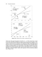
In Figure 19 [20], the effect of wind and wave loads on the bending moments at the tower–spar interface of CMS wind turbine
for different mean wind speeds is illustrated. The statistical characteristics are based on five 1 h samples. The maximum responses
correspond to the up-crossing rate of 0.000 1 and are obtained by extrapolation. The up-crossing rate of a process at a defined level is
the frequency of passing that level. The up-crossing rate of 0.000 1 for a process at a defined level means that the process (e.g.,
structural response) passes that level by a rate of 0.000 1 (Hz). For higher response levels, the up-crossing rate is lower. The
maximum responses for an FWT can happen in storm condition. However, for an onshore wind turbine, the maximum responses
are linked to the rated wind speed load cases. The responses of an FWT in survival conditions are mainly governed by wave loads.

2.09.5.2.3

Servo-induced negative damping

The blade pitch control of an operating turbine can introduce negative damping in an FWT. For example, if the relative wind speed
experienced by the blades increases due to the rigid body motion of the system, then, if a conventional controller is used, the blades
will feather to maintain the rated electrical power. Thus, the thrust force will decrease, which will introduce negative damping for
overrated wind speed load cases. However, this is not the case in fixed wind turbines since the frequency of the blade pitch controller
is normally less than the frequencies associated with the relative rotor motions induced by the structural responses.
Figure 20 [21] shows the comparison between the nacelle surge motion of TLS wind turbine with the untuned and tuned

controller to avoid negative damping in the overrated constant wind condition (V = 17 m s−1, HS = 4.2 m, and TP = 10.5) for a
downwind TLS. This is an example to highlight the servo-induced loads. The tuned controller has much lower pitch resonant


Mechanical-Dynamic Loads

261

4.0E+05
Parked wind turbine
Operating wind turbine

3.5E+05

Bending moment (kNm)

3.0E+05

Mean (Turbulent wind)
STD (Turbulent wind)
Max (Turbulent wind)

2.5E+05

Mean (Constant wind)
STD (Constant wind)

2.0E+05

Max (Constant wind)

1.5E+05
1.0E+05
5.0E+04
0.0E+00
6

10

14

18

22

26

30

34

38

42

46

50

Mean wind speed (m sec−1)
Figure 19 Bending moment at the tower–spar interface of CMS wind turbine (wave- and wind-induced) for constant and turbulent wind cases. The statistical

characteristics are based on five 1 h samples. The maximum responses correspond to the up-crossing rate of 0.000 1 and are obtained by extrapolation.
Reproduced with permission from Karimirad M and Moan T (2011) Wave and wind induced dynamic response of catenary moored spar wind turbine. Journal
of Waterway, Port, Coastal, and Ocean Engineering.

50

Untuned
Tuned

45
Pitch response instability
due to servo-induced
negative damping

40

S (m2 s rad–1)

35
30
25
20
15

Wave frequency response

10
5
0

0

0.5

1
Frequency (rad s–1)

1.5

2

Figure 20 Nacelle surge spectra of TLS wind turbine, with the untuned and tuned controller in the overrated constant wind condition (V = 17 m s−1,
HS = 4.2 m, and TP = 10.5). The motion response instabilities due to servo-induced negative damping. Reproduced with permission from Karimirad M and
Moan T (2011) Ameliorating the negative damping in the dynamic responses of a tension leg spar-type support structure with a downwind turbine.
European Wind Energy Conference EWEC 2011. Brussels, Belgium, 14–17 March.

response. In the overrated wind speed range and due to the negative damping effect of the controller, the pitch resonant was
dominant. After tuning the controller gains, the pitch resonant response is positively damped out.

2.09.5.2.4

Comparison of power production of TLS and CMS turbines

Figure 21 shows the power production of CMS and TLS FWTs. The properties of the two systems are defined in Tables 4 and 5. The
electrical power produced by these FWTs is close. However, to compare the concepts it is necessary to consider other parameters such


262

Mechanical-Dynamic Loads

6

Power (MW)

5
4
3
Catenary moored spar
Tension leg spar

2
1
0
6

8

10

12

14

16

18

Mean wind speed (m s–1)

Figure 21 Comparison of power production of TLS and CMS offshore wind turbines.

as structural responses, fatigue life, and cost of produced electricity. The cost should include the design, construction, installation,
maintenance, operation, and other practical issues.

2.09.6 Conclusions
The fast development of wind technology has introduced new challenges for researchers. This includes larger wind turbines with
more elastic responses, floating and fixed offshore wind turbines with comprehensive dynamic loads, innovative concepts, and
similar aspects. Advanced aero-hydro-servo-elastic numerical tools are needed to perform integrated analysis for today’s wind
turbines. This chapter made an introduction to mechanical-dynamic loads for both onshore and offshore wind turbines with a focus
on the wave- and wind-induced loads to assess the structural integrity and power performance of FWTs. Several case studies were
provided for both fixed and FWTs to support the presented discussion.

Appendix A: Environmental Conditions
To design, install, and operate wind turbines in a safe and efficient manner, it is necessary to have realistic metocean (meteorological
and oceanographic) data available for the conditions to which the installation may be exposed.

A.1

General

The first step in performing rational structural dynamic analysis is setting realistic environmental conditions. The most important
for a wind turbine are the wind and wave at the wind park site. However, at some offshore locations, other parameters may be
important (e.g., air and sea temperature, tidal conditions, current, and ice conditions).
The wave and wind are random in nature. This randomness should be represented as accurately as possible to calculate
reasonable hydro-aero-dynamic loading. Both the waves and the wind have long-term and short-term variability. The simulation
time depends on the natural periods of the system. Wave-induced motions of common floating structures have been carried out
considering a 3 h short-term analysis [22]. In wind engineering, the 10 min response analysis can cover all the physics governing a
fixed wind turbine. When it comes to FWTs, the correlation between the wave and wind should be accounted for. For each
environmental condition, the joint distribution of the significant wave height, wave peak period, wave direction, and mean water

level (MWL, relevant for shallow water) combined with the mean wind speed, wind direction, and turbulence should be considered.

A.2

Joint Distribution of Wave Conditions and Mean Wind

The wave and wind show long-term and short-term variability. The long-term variability of the wind can be defined by the mean wind
speed and direction. The short-term variability of the wind is usually defined by the turbulence. In an offshore site, the ocean waves can be
wind-generated and swell. The waves are usually defined by the peak period and significant wave height. The correlation between the
waves and wind should be considered for stochastic analysis of FWTs. Site assessments containing metocean data are needed to develop
the joint distribution of the waves and wind for the analysis. The joint distribution can include the wave and wind characteristics, such as
the mean wind speed, turbulence, direction of the waves and wind, significant wave height, and wave peak period. However,
development of the joint distribution requires measurement of simultaneous wave and wind time histories at the offshore sites for
several years. Currently, limited site assessments considering the correlated wave and wind time series are available. These data are
missing the correlation between the turbulence and wave/mean wind characteristics. The offshore wind turbine is a new technology, and
large metrological/oceanological studies for determining the proper joint distribution of wave and wind characteristics are needed.


Mechanical-Dynamic Loads

263

Weibull PDF (Hs|V)

0.5
0.4
0.3
0.2
0.1
0

0
20
V (m s–1)

40

15

5

10

0

Hs (m)

Figure 22 The Weibull probability density function of the significant wave height (HS) given the mean wind speed at the nacelle (V) for the Statfjord
offshore site at 59.7°N and 4.0°E and 70 km from the shore.

In this chapter, the wind and wave were assumed to have the same direction. The correlation between the mean wind speed,
significant wave height, and wave peak period was considered, which can be done by fitting the analytical functions to the site
assessments by considering a mathematical distribution for the mean wind speed and significant wave height. It is possible to
model the significant wave height as a Weibull distribution whose parameters were functions of the mean wind speed [23].
Figure 22 illustrates the Weibull probability density function of the significant wave height (HS) given the mean wind speed at the
nacelle (V) for the representative offshore wind park, Statfjord offshore site at 59.7°N and 4.0°E and 70 km distance from the shore.
The significant wave height increased with the increase of the wind speed. For higher wind speeds, the Weibull distribution was
negatively skewed. For each wind speed, a range of significant wave heights was possible. Smaller wind speeds had a narrower range
of significant wave heights. The IEC 61400-3 standard recommends the use of the median significant wave height at each wind
speed for dynamic response analysis of offshore wind turbines.

Appendix B: Wind Theory
The wind varies over space and time. It is important to know these variations to investigate the site energy resources for making
electrical power, which is the first concern for a specific location. The spatial and temporal variations of the wind are defined as [24]:
Spatial variations:
•
•
•
•
•

Trade winds emerging from subtropical, anticyclonic cells in both hemispheres
Monsoons, which are seasonal winds generated by the difference in temperature between land and sea
Westerlies and subpolar flows
Synoptic-scale motions, which are associated with periodic systems such as travelling waves
Mesoscale wind systems, which are caused by differential heating of topological features and called breezes.

Time variations:
•
•
•
•

Long-term variability, which are annual variations of wind in a special site
Seasonal and monthly variability
Diurnal and semidiurnal variation
Turbulence (range from seconds to minutes).

The temporal variations are usually represented by the energy spectrum of the wind. In Figure 23, the Van der Hoven wind speed
spectrum [25] is shown. The yearly wind speed changes, pressure systems, and diurnal changes are influencing the left side of the
wind speed spectrum. However, the turbulence shows itself in the right side of the spectrum.

The wind is characterized by its speed and direction. The wind energy is concentrated around two separated time periods
(diurnal and 1 min periods), which allows the splitting of the wind speed into two terms: the quasi-steady wind speed
(usually called the mean wind speed) and the dynamic part (the turbulent wind). In other words, the time-varying wind
speed is considered to be made up of a steady value plus the fluctuations about this steady value. The steady value is
assumed to be quasi-static; thus, its time dependency is negligible for the current purpose (the probabilistic dynamic
response analysis). The long-term probability distribution of the mean wind speed is predicted by fitting site measurements
to the Weibull distribution (eqn [16]). The Weibull probability density function (fW) shows that the moderate winds are
more frequent than the high-speed winds.


264

Mechanical-Dynamic Loads

ωSV (ω) ((m s–1)2)

6

4

2

0
0.001

0.01
4 days

0.1
semidiurnal

1

10
5 min

100

1000 cycles h–1
5s

Figure 23 Van der Hoven wind speed spectrum. Reproduced with permission from Bianchi DF, Battista HD, and Mantz RJ (2007) Wind Turbine Control
Systems. Germany: Springer.

0.12
Onshore, k = 1.75 and c = 7.3
Coast, k = 2 and c = 9
Offshore, k = 2.2 and c = 11.3

0.1

Probability(–)

0.08

0.06

0.04

0.02

0

0

5

10

15
Wind speed (m s–1)

20

25

30

Figure 24 Weibull probability distribution of wind velocity for three different sites: onshore, coastal, and offshore considering typical values of shape and
scale parameters. Reproduced with permission from Twidell J and Gaudiosi G (2008) Offshore Wind Power. Essex, UK: Multi-Science Publishing Co Ltd.

kw
fWðV Þ ¼
cw

�

V
cw

�kw − 1

�

V
exp −
cw

�kw !

½16Š

where V is the wind speed, kw is the shape parameter describing the variability about the mean, and cw is a scale parameter related to
the annual mean wind speed. In Figure 24, the Weibull probability distribution for three different areas, that is, onshore, coastal,
and offshore, with typical values of shape and scale parameters is plotted [7].
An empirical formula for the annual mean wind speed (VAnnual) is given in eqn [17] by Lysen [26].
VAnnual ¼ cw ð0:568 þ 0:433= kw Þ1=kw

½17Š
−1

The annual mean wind velocities corresponding to different sites in Figure 24 are 6.5, 8, and 11.3 m s for the onshore, coastal, and
offshore sites, respectively. Considering the ratio between the offshore and onshore power corresponding to the present example
can be up to 5, which confirms the possibility of generating more electrical power by moving offshore.
The mean wind speed is a function of height, which can be represented by different shear models such as the Prandtl logarithmic
and power laws. In these mathematical models, a parameter called the roughness length or exponent accounts for the effect of the
type of surface over which the wind blows [12].
The turbulence in the wind is caused by the dissipation of the wind kinetic energy into thermal energy via the creation and
destruction of progressively smaller eddies or gusts. Turbulent wind may have a relatively constant mean over time periods of an
hour or more, but over shorter times (minutes or less) it may be quite variable. Turbulent wind consists of longitudinal, lateral, and

vertical components [13].


Mechanical-Dynamic Loads

265

120
Offshore, V = 49 m s−1, I = 0.10
Onshore, V = 49 m s−1, I = 0.15
Offshore, V = 17 m s−1, I = 0.15
Onshore, V = 17 m s−1, I = 0.20

Spectrum ((m s–1)2 rad–1 sec–1)

100

80

60

40

20

0

0

0.1

0.2

0.3

0.4

0.5

Frequency (rad

0.6

0.7

0.8

0.9

1

s–1)

Figure 25 Kaimal spectra for onshore and offshore sites under operational and extreme environmental conditions, with the corresponding mean wind
velocities and turbulence intensities for those conditions.

The dynamic part of the wind speed, turbulence, includes all wind speed fluctuations with periods below the spectral gap. The
spectral gap occurs around 1 h, which separates the slowly changing and turbulent ranges. Therefore, all components in the range
from seconds to minutes are included in the turbulence. The captured annual power is not affected by turbulence very much, but the
turbulence has a major impact on aero-elastic structural response and electrical power quality. It is common to describe the wind

turbulence in a given point in space using the power spectrum. The Kaimal and von Karman spectra are widely used. Both models
depend on the mean wind speed and the topography of the terrain. One useful parameter is the turbulence intensity, which is
defined as the ratio of the standard deviation of the wind speed to the mean wind speed. The turbulence intensity decreases with
height. The turbulence intensity is higher when there are obstacles in the terrain; hence, the turbulence intensity for an offshore site
is less than that for a land site.
The turbulent wind spectrum, such as the Kaimal spectrum (eqn [18]), is a function of the frequency, turbulence intensity, and
mean wind speed [27].
Sðf Þ ¼ �

It2 V10 min l
1þ1:5

f l

�5=3

½18Š

V10 min

where It = σ / V10 min is the turbulent intensity, f is the frequency in hertz, V10 min is the 10 min averaged wind speed, and l is a length
scale. l = 20 hagl for hagl < 30 m or l = 600 m otherwise where hagl is the height above ground level.
In Figure 25, the Kaimal spectra for onshore and offshore sites are plotted. The harsh and operational environmental conditions
with their mean wind speed and turbulence intensity were considered. The spectrum under harsh conditions has much more energy
compared to those under operational conditions, especially in the low frequency region. At the offshore site, the wind is steadier,
and the turbulence is decreased, but at onshore sites, the obstacles in the terrain influence the boundary layer and make the wind
more turbulent.

Appendix C: Wave Theory
In this section the regular wave theory, modified regular wave theory, and irregular wave theory are described.

C.1

Regular Wave Theory

In the regular wave theory, the wave is assumed to be sinusoidal with constant wave amplitude, wavelength, and wave period. Thus,
the regular propagating wave is defined as ζ = ζa sin(ωt − kx). ζ is the time- and position-dependent wave elevation. The linear wave
theory, usually called the Airy theory, can be used to represent the wave kinematics. In the Airy theory, the seawater is assumed to be
incompressible and inviscid. The fluid motion is irrotational. Then, a velocity potential exists and satisfies the Laplace equations. By


266

Mechanical-Dynamic Loads

applying the kinematic boundary conditions and the dynamic free-surface conditions, the velocity potential, and the wave
kinematics can be found [16]. Based on the Airy theory, the horizontal water particle kinematics are described by eqns [19] and
[20]. The dynamic pressure is presented in eqn [21].
u ¼ ωζ a

cosh kðz þ hÞ
sinðωt − kxÞ
sinh kh

aX ¼ ω 2 ζ a

cosh kðz þ hÞ
cosðωt − kxÞ
sinh kh

½19Š
½20Š

where u and aX are the water particle velocity and acceleration in the x-direction (wave propagation direction), respectively, ω is the
wave frequency, ζa is the regular wave amplitude, k is the wave number, the z axis is upward, and h is the mean water depth.
PD ¼ ρw gζ a

cosh kðz þ hÞ
sinðωt − kxÞ
cosh kh

½21Š

In deepwater, the water particles move in circles in accordance with the harmonic wave. In deepwater, the depth is greater than half
of the wavelength (h ≥ λ/2). Thus, the effect of the seabed cannot disturb the waves. For shallow water, the effect of the seabed
transforms the circular motion into an elliptic motion.
When the wave amplitude increases, the wave particle no longer forms closed orbital paths. In fact, after the passage of each crest,
particles are displaced from their previous positions. This phenomenon is known as the Stokes drift. The Boussinesq equations that
combine frequency dispersion and nonlinear effects are applicable for intermediate and shallow water. However, in very shallow
water, the shallow water equations may be used.
Linear wave theory represents the first-order approximation in satisfying the free-surface conditions. It can be improved by
introducing higher-order terms in a consistent manner via the Stokes expansion [16]. In this chapter, the linear wave theory was
applied.
The wave theory discussed here is just applicable for nonbreaking waves. The wave breaks when H/h ≥ 0.78 in shallow water and
when H/λ ≥ 0.14 in deepwater [8]. H is the wave height and the h is the mean water depth. For extreme waves, when the height
increases greatly, the nonlinear features of the wave kinematics cannot be captured through linear wave theory. However, the
nonlinear methods are mainly applicable for deterministic waves; they are not suitable for stochastic wave fields. Fortunately, the
probability of breaking waves is relatively small. Moreover, most of the waves break close to the coast and not at the offshore wind
turbine site.

C.2

Modified Linear Wave Theory

The Airy wave theory is only valid up to the MWL surface and does not describe the kinematics above that level. Different
mathematical models, such as constant stretching and Wheeler stretching, have been suggested to describe the wave kinematics
above the MWL surface. In the constant stretching model, it is assumed that the wave kinematics are constant above the MWL. In the
Wheeler stretching model, the vertical coordinate z is substituted by the scaled coordinate z′ (eqn [22]). In this chapter, the Wheeler
stretching model was used.
z′ ¼ ðz − ζ Þ

h
hþζ

½22Š

where ζ is the wave elevation and ζ = ζa sin(ωt − kx). In the following section, the stretching in the stochastic context is explained.

C.3

Irregular Wave Theory

Wind-generated waves are forced waves that are sustained by receiving energy from the wind. Swell waves are free waves that
do not receive wind energy due to the absence of wind or movement to a new free-wind location. The practical way to model
ocean waves in ocean engineering assumes that the sea surface forms a stochastic wave field that can be assumed to be
stationary in a short-term period. The stationary assumption of the wave is site-dependent [22]. For most practical offshore
engineering purposes, this assumption works very well and gives good agreement with full-scale measurements. The wave field
is assumed to be Gaussian, which gives a reasonably good approximation of reality in most cases. The stochastic model
approved for the waves leads to a normally distributed water surface elevation. The wave crests follow the Rayleigh distribution
if the wave elevation is assumed to be Gaussian and narrow-banded. However, some phenomena, such as slamming, can

violate the Gaussian assumption.
Based on the Gaussian assumption, the stationary sea (represented by the wave elevation at a point in space) can be modeled by
a wave spectrum. The Pierson–Moskowitz (PM) and Joint North Sea Wave Project (JONSWAP) spectra (eqns [23] and [24]) are
examples of mathematical models to represent the ocean wave spectrum. For a fully developed wind sea, the PM spectrum can be
used, and for a growing wind sea, the JONSWAP [28] spectrum can be used. Moreover, the Torsethaugen spectrum (two-peaked
wave spectrum) is introduced to define a sea comprising wind-generated waves and swells.


Mechanical-Dynamic Loads

267

90
Operational condition, HS = 4.2 m and TP = 10.5 sec
Harsh condition, HS = 14.4 m and TP = 13.3 sec

80

Spectrum (m2 /rad/sec)

70
60
50
40
30
20
10
0

0

0.2

0.4

0.6

0.8

1

1.2

Frequency (rad/sec)
Figure 26 The JONSWAP wave spectrum for harsh and operational conditions.

SPM ðf Þ ¼

�
�
5 HS2
5
− 4
Þ
−
ð
exp
f
T
P

4
16 TP4 f 5

where HS is the significant wave height, TP is the wave peak period, and f is the frequency in hertz.
!
− ðf − f P Þ 2
SJS ðf Þ ¼ Fn SPM ðf Þ γJS exp
2 σ 2JS f 2P
(
σ JS ¼

σ a for f ≤ f P ðtypically : 0:07Þ
σ b for f > f P ðtypically : 0:09Þ

� �
�� − 1
Fn ¼ 5 0:065 γ0:803
þ 0:135
JS

for 1 ≤ γJS ≤ 10

½23Š

½24Š

½25Š
½26Š

where γJS is the wave spectrum shape parameter, which is around 3.3 for seas that are not fully developed. For fully developed seas,

γJS is taken to be 1. Therefore, the JONSWAP and PM spectra are the same for γJS =1. fP = 1/TP is the wave peak frequency in hertz.
In Figure 26, the JONSWAP wave spectrum for operational and harsh environmental conditions is illustrated. The extreme
sea state has much larger peaks, and it also covers a wider range of frequencies. The peak frequency of a harsh sea state is
shifted to lower frequencies as well. This shift means that the probability of resonant motion occurrence is higher in extreme
environmental conditions.
For a suitable wave spectrum representing the offshore site, the calculations may begin by converting the spectrum back into
individual sinusoids using inverse fast Fourier transformation. Each sinusoid has a frequency and amplitude that can be derived
from the energy density given by the wave spectrum. The phase angle is assigned randomly to each sinusoid.
In the stochastic context, the Wheeler stretching can be applied as well. For each regular wave, the stretching is applied, and the
wave kinematics over the MWL is obtained. Then, the wave elevation, the velocities, and acceleration of regular waves are added
together to obtain the irregular wave elevation, velocity, and acceleration for that particular time.

References
[1] Sclavounos PD, Lee S, DiPietro J, et al. (2010) Floating offshore wind turbines: Tension leg platform and taught leg buoy concept supporting 3–5 MW wind turbines. European
Wind Energy Conference (EWEC). Warsaw, Poland, 20–23 April.
[2] Henderson AR, Leutz R, and Fujii T (2002) Potential for floating offshore wind energy in Japanese waters. ISOPE Conference. ISBN 1-880653-58-3, Kitakyushu, Japan, 26–31
May.
[3] IEA (2008) Renewable Energy Essentials: Wind. (Accessed June 2010).
[4] Jonkman J (2009) Dynamics of offshore floating wind turbines-model development and verification. Wind Energy 12(5): 459–492.
[5] Jonkman J (2007) Dynamics modeling and loads analysis of an offshore floating wind turbine. NREL, Technical Report, NREL/TP-500-41958. Golden, CO: NREL.