Technical efficiency and its determinants the case of manufacturing firms in vietnam
Bạn đang xem bản rút gọn của tài liệu. Xem và tải ngay bản đầy đủ của tài liệu tại đây (2.17 MB, 79 trang )
UNIVERSITY OF ECONOMICS
HO CHI MINH CITY
VIETNAM
INSTITUTE OF SOCIAL STUDIES
THE HAGUE
THE NETHERLANDS
VIETNAM- NETHERLANDS
PROGRAMME FOR M.A IN DEVELOPMENT ECONOMICS
TECHNICAL EFFICIENCY AND ITS
DETERMINANTS: THE CASE OF
MANUFACTURING FIRMS IN VIETNAM
A thesis submitted in partial fulfilment of the requirements for the degree of
MASTER OF ARTS IN DEVELOPMENT ECONOMICS
I~
By
TRAN VAN KHUE
Academic Supervisor:
DR. NGUYEN TRONG HOAI
DR. PHAM LE THONG
HO CHI MINH CITY, DECEMBER 2011
I
I
:
-~
~
ABBREVIATIONS
AEC
Allocative Efficiency Change
DEA
Data Envelopment Analysis
E&E
Electrical and Electronics
FDI
Foreign Direct Investment
FEM
Fixed Effects Model
GDP
Gross Domestic Product
GSO
General Statistic Office
ICT
Information and Communication Technology
MDE
Master of Development Economics
POLS
Pooled Ordinary Least Squares
R&D
Research and Develop
REM
Random Effects Model
SEC
Scale Economies
SEC
Scale Efficiency Change
SFPF
Stochastic Frontier Production Function
SMEs
Small and Medium Enterprises
SOEs
State-Owned Enterprises
TE
Technical Efficiency
TEC
Technical Efficiency Change
TFP
Total Factor Productivity
TP
Technical Progress
TT
Time Trend
III
TABLE OF CONTENTS
CHAPTER 1: INTRODUCTION
1.1 The problem statement ................................................................................. 2
1.2 Objectives of the research ............................................................................. S
1.3 Research questions ....................................................................................... 6
1.4 Research methodology .................................................................................. 6
1.5 Thesis structure ............................................................................................. 7
CHAPTER 2: LITERATURE REVIEW
2.1 Introduction .................................................................................................. 8
2.2 Basic Concepts and Theoretical Review ...................................................... 8
2.2.1 The Production Function .............................................................................. 8
2.2.2 Cobb-Douglas production function .............................................................. 9
2.2.3 Technical Efficiency .................................................................................... 11
2.2.4 Technical efficiency measurement .............................................................. 12
2.2.5 The stochastic frontier production function (SFPF) ...................................... 13
2.3 Empirical Studies .......................................................................................... 16
2.3.1 Studies in advanced countries ....................................................................... 16
2. 3. 2 Studies in developing countries .................................................................... 19
2.3.3 Studies in Vietnam ....................................................................................... 22
2.4 Analytical framework for the research ........................................................ 29
CHAPTER 3: RESEARCH METHODOLOGY AND DATA COLLECTION
3.1 Introduction .................................................................................................. 31
3.2 Research methodology .................................................................................. 31
3.2.1 The stochastic frontier model ...................................................................... .31
3.2.2 The technical efficiency model.. ................................................................... 34
3.3 Testing Hypothesis ........................................................................................ 37
3.3.1 The stochastic frontier model ....................................................................... 37
IV
3.3.2 The technical efficiency model.. ................................................................... 37
3.4 Data Collection .............................................................................................. 38
CHAPTER 4: ANALYSIS RESULTS
4.1 Sample profile ............................................................................................... 39
4.2 Technical efficiency ....................................................................................... 41
4.3 Comparison of technical efficiency ............................................................. 44
4.4 Technical efficiency model ............................................................................ 46
4.4.1 Testing for the most appropriate model ....................................................... .46
4.4.2 Testing for heteroskedasticity ...................................................................... .47
4.4.3 Determinants of technical efficiency ........................................................... .4 7
4.5 Chapter Summary ........................................................................................ 50
CHAPTER 5: CONCLUSIONS, RECOMMENDATION AND LIMITATIONS
5.1 The conclusions ............................................................................................. 51
5.2 The recommendations ................................................................................... 54
5.3 Limitations .................................................................................................... 55
REFERENCES ................................................................................................... 56
APPENDICES ..................................................................................................... 60
v
LIST OF TABLES & GRAPHS
Table 2.1: Summary of Empirical Studies
Table 3.1: Summary ofvariables in the frontier production function
Table 3.2: Summary of variables in the technical efficiency model
Table 4.1: Descriptive statistics of output, capital and labour of manufacturing firms
in the period 2000-2004
Table 4.2: Estimates ofti model and tvd model
Table 4.3: The statistical tests of some hypothesis
Table 4.4: Summary of technical efficiency between ti model and tvd model
Table 4.5: Determinants oftechnical efficiency
Graph 4.1: The structure of 1,645 manufacturing firms from other sectors
VI
------
LIST OF FIGURES
Figure 1.1: The share of manufacturing enterprises in all industries ofVietnam
Figure 2.1: Illustration of Technical Efficiency
Figure 2.2: Analytical Framework
VII
CHAPTER 1: INTRODUCTION
1.1 The problem statement
Since the launch of renovation in 1986, Vietnam has successfully transformed the
centrally-planned economy into a market economy and made great achievements in
social and economic aspects. In the period of 2000- 2010, the country's economic
growth was relatively high and stable at an annual average rate of 7.2%. In 2010,
the real GDP was recorded 3.4 times as much as that in 2000; the state budget
collection was 5 times; and the GDP per capita stood at US$1,168 (GSO, 2011). By
achieving these, Vietnam has moved from the group of poorest countries to the
group of middle-income countries. In addition, Vietnam has been successful in
poverty reduction, close to achieving universal primary education, improving
maternal health, reducing child mortality, obtaining much progress in gender
equality and empowering women, and etc.
In contribution to economic and social development, Vietnamese enterprises play a
crucial role. Business activities of enterprises have made significant progress. In
1995, enterprises contributed about 45.3% of GDP; in 2001 this share increased to
•
53.2% and in 2007 was over 60% (GSO, 2008). The development of enterprises in
many different sectors and localities lead to the change of economy's structure
which reduces the share of agriculture and increases those rates of industry and
services.
With regards to manufacturing enterprises, they made important contribution to
dealing with social matters such as creating more new jobs, increasing income for
employees, contributing more to the state budget, and etc. In more details,
manufacturing enterprises create 2.203 million jobs, accounting for 47.3% of total
jobs in all enterprises (GSO, 2007).
However, many weaknesses are found in the process of the development of the
economy in general and the manufacturing sector in particular. The infrastructure
has not been completed and needs to be improved comprehensively. The shortage
2
of electricity and water which are common may reduce the productivity (Klause et
al., 2005). So, the efficiency and competitiveness of the economy still is lower than
its potential.
Moreover, the performance of enterprises has different results because of their
resource, types of ownership, type and scale of business, location and some other
reasons. Although the business environment has been more transparent and flexible
for business operation, the business results of each enterprise might not grow
steadily. In general, Vietnam enterprises expose their own features.
Firstly, the number of new enterprises especially private companies has grown
sharply since 2000 when the Enterprise Law carne into effect. In three years after
the issue of the Law, more than 72,600 new private enterprises were established,
creating around 1.6 - 2 million new jobs (ClEM, 2004). These figures are very
impressive when compared with just 26,000 private enterprises operating by the end
of 1998.
Secondly, enterprises located in big cities such as Hanoi; Hochirninh city may enjoy
many favorable conditions such as ideal geographical location; advantage of
telecommunication, transportation; abundant labor supply with high skill to apply
new technology in production. Consequently, the number of enterprises in these
cities increases very fast and accounts for about 47% of total number of enterprises
and 45% of total revenue of the whole country (GSO, 2007). On the other hand,
these enterprises are still facing with a lot of problems such as non-synchronous
infrastructure, un-skilled labor. Especially, each enterprise in big cities has to
compete fiercely with many other local and domestic companies located at the same
city. These problems in association with improper policies might cause the
companies to slowly increase their effectiveness.
Thirdly, as a multi-sector market model operating according to the market
mechanism and the state regulations, Vietnam's enterprises include state, private
and foreign-invested sectors where the former plays a leading role in the economy.
3
The government uses the state enterprises as an important tool to stabilize the microeconomic environment and market prices of essential commodities such as electricity,
coal, transport, rice and rubber. So, state enterprises have received a lot of support,
priorities, and subsidies from government. Therefore, the performance of state
enterprises is questioned about the efficiency relative to other sectors in the economy.
For above reasons, some issues need to be clarified such as the performance of firms
in Vietnam;
the production efficiency level of firms located in former Hanoi,
Hochiminh cities and other places; firms of the state, foreign and other sectors; and
the factors influencing the technical efficiency of firms.
The purpose of this thesis is to identify the above issues. And, the manufacturing
sector is selected to research because of following reasons: The share of
manufacturing enterprises in all industries accounts more than 20 percent of all kind
of activity (GSO, 2006). However, manufacturing enterprises contribute important
shares of revenue (more than 30 percent), number of employees (about 50 percent)
and export value (22 percent).
The thesis applies a stochastic frontier production model and technical efficiency
model to analyze the technical efficiency of manufacturing firms and try to find the
determinants that affect firms' technical efficiency.
4
Figure 1.1: The share of manufacturing enterprises in all industries of
Vietnam
60
50
tn
,-=
Q)
·c 40
.5 30
Employment
C'G
Export
.5 20
';te
10
0
2000 2001 2002 2003 2004 2005 2006
Source: GSO
1.2 Objectives of the research
Basically, this thesis aims at four objectives as follows:
(1) To measure the level of technical efficiency of manufacturing firms in the
period 2000 to 2004.
(2) To compare the difference in technical efficiency between manufacturing
firms located in former Hanoi and Hochiminh City and those located in other
provinces; between firms of state-owned, foreign firms and other firms.
(3) To identify factors influencing the technical efficiency of manufacturing
firms.
(4) To suggest appropriate policies for improving technical efficiency of
manufacturing firms.
*Note: Former Hanoi: Because the data applied in the thesis from 2000 to 2004. Since August
1, 2008 Hanoi has merged with Hatay province and parts of neighboring of Vinhphuc and
Hoabinh provinces.
5
1.3 Research questions
With the research objectives, the thesis is therefore going to answer the following
questions:
(1) What is the level oftechnical efficiency of manufacturing firms?
(2) What are differences in technical efficiency of manufacturing enterprises
located in former Hanoi*, Hochiminh city and other provinces; state-owned,
foreign and other firms?
(3) What are factors affecting the technical efficiency of manufacturing
firms?
1.4 Research methodology
The descriptive statistics, quantitative analysis are used to solve with the research
questions.
The stochastic frontier production model in the form of Cobb-Douglas production
function is applied to estimate and measure the technical efficiency of
manufacturing companies. Then technical efficiency is compared between the group
of manufacturing firms located in former Hanoi, Hochiminh city and other places;
between state and foreign with other groups of manufacturing firms.
In the second stage, the thesis examines factors influencing the technical efficiency
of enterprises. For the data with two dimensions time series and cross sections, the
thesis uses the panel data analysis via the appropriate method from pooled Ordinary
Least Squares (OLS), Random Effects Model (REM) and Fixed Effects Model
(FEM).
The data set applied for this thesis comes from the Vietnam Enterprise Survey
conducted by the General Statistic Office in the period 2000- 2004.
6
1.5 Thesis structure
The thesis is presented in five chapters. After this chapter the rest of this thesis will
be presented in four chapters. Chapter 2 covers the literature about the production
function, technical efficiency, the stochastic frontier production function and
empirical studies. Chapter 3 presents the research methodology and data. Chapter 4
presents the research results. Finally, chapter 5 gives conclusions, recommendations
and limitations ofthe study.
7
CHAPTER 2: LITERATURE REVIEW
2.1 Introduction
This chapter provides an overview of literature about the research problems in a
logical manner in order to drive this thesis into a correct direction. This chapter is
divided into four sections. The first section presents the basic concepts and
theoretical review which includes production functions, Cobb-Douglas production
function, technical efficiency, technical efficiency measurement and the stochastic
frontier production function. The second section gives various empirical studies
about technical efficiency to provide the foundation for developing the analytical
model of this thesis. The final section summarizes theoretical and empirical review
and proposes the applied models in this thesis.
2.2 Basic Concepts and Theoretical Review
2.2.1 The Production Function
A production function is the technical relationship between the quantities of
productive factors used and the amount of products obtained from every
combination of factors, assuming that the most efficient available methods of
production are used.
A general production function can be written as:
(2.1)
Where:
Q is the quantity of output
X~>
Xz, ... , Xn are the quantity of factor inputs such as capital, labor, raw materials,
etc.
8
Technically, the production function depicts the maximum output that can be
produced by the input combination, given the technology in use. In production, the
inputs can be changeable and substitutable.
Although the relationship between output and inputs is fundamentally physical,
production function often uses monetary values. The production process uses
several types of inputs that cannot be aggregated in physical units. It also produces
several types of output Goint production) measured in different physical units. One
of the ways to deal with the multiple output case is to aggregate different products
by assigning price weights to them (Mishra, 2007).
There are many kinds of production function that can be used in empirical studies as
follows:
- Linear production function is a function that assumes a perfect linear relationship
between inputs and total output.
- Leontief production function is a function that assumes the inputs are used in fixed
proportions.
- Cobb-Douglas production function is a function that assumes some degree of
•
substitutability between inputs.
- Other production functions such as quadratic, transcendental-logarithm (translog),
and etc.
2.2.2 The Cobb-Douglas production function
The most widely utilized functional form for econometric modeling is the CobbDouglas form. This form is the most popular one in applied research, because it is
easy to handle mathematically.
The Cobb-Douglas production function with two inputs of labor and capital is as
follows:
9
(2.2)
Where
Y is total production (the monetary value of all goods produced in a year)
L is the labor input
K is capital input
A is total factor productivity or the technology state
a and
~
are the output elasticities of labor and capital, respectively. These values are
constant, determined by available technology.
Output elasticity measures the responsiveness of output to a change in levels of
either labor or capital used in production.
lfa+~=l
Ifa+~
: constant returns to scale;
: decreasing returns to scale;
And if a + ~ > 1: increasing returns to scale.
•
There some methods estimating the parameters of a Cobb-Douglas production
function and the typical estimation is based on the linear equation. From equation
2.2, taking the logs of both sides, the function is transferred as log-linear form as
follows:
log Yi = log A + a log Li + ~ log Ki
(2.3)
Where
Y, A, Land K are as defined earlier
The residual from estimation of function 2.3 is a random error term or a disturbance
term named Ui. The disturbance U is different for each firm and assumed to have
normal distribution.
10
2.2.3 Technical Efficiency
According to Farrell (1957), total economic efficiency includes two components
that are technical efficiency and allocative efficiency.
Technical efficiency is defined as the firm's ability to maximize the output from a
given set of inputs (output-increasing oriented) or the firm's ability to minimize
inputs used for a given set of output (input-saving oriented) (Koopmans, 1951).
Allocative efficiency displays the firm's ability to use inputs in optimal proportion
given their market prices and the production technology they used.
And, figure 2.1 shows more clearly about the relation of technical efficiency and
scale efficiency. The ABC line represents the frontier for the production process.
Points are on the frontier showing the maximum pure technical efficiency.
Meanwhile, the through-origin line expresses the scale efficiency and the points are
on the line have constant returns to scale. Scale efficiency is used to indicate
whether or not a firm is operating at an optimal scale. A firm, that has a technical
efficiency, may be due to purely technical efficiency or scale efficiency
Points A, B, C, D and E present the combination of a certain levels of input and
output. Observations of A, B and C are on the frontier line, so they have purely
technical efficiency. Meanwhile, observations D and E are below the frontier line.
The tangential line at point B expresses the constant returns to scale of technology.
The point B shows the relative technical efficiency. In other words, at this point,
firm obtains both purely technical efficiency and scale efficiency due to its location
on the frontier and the constant returns to scale.
Observations A and C are on the frontier so they are purely technical efficiency.
However, these points are not efficient in scale.
Observation D is inefficient in both scale and technique. Theoretically, the same
level of input could be used to achieve a higher level of output, at point D the firm
can move to the frontier between points B and C.
II
Observation E is purely technical inefficient because it lies below the frontier; but it
is scale efficient because it produces at input level of x2 the scale efficient level of
input at the same level of scale efficiency of point B.
Figure 2.1 Illustration of technical efficiency
Output (:y)
y;
y~~
·- ... -· - - - -
x,
Input tx)
2.2.4 Technical efficiency measurement
So far the firm's technical efficiency has been analyzed by many researchers.
Among various methods, the two following ones are frequently applied: the
parametric approach called stochastic frontier production function - SFPF and the
non-parametric approach or data envelopment analysis - DEA.
A stochastic frontier production function approach is used to estimate a production
function when the specification of technology is given. In other words, the estimated
production function can be used for all firms of the same sector. In SFPF, the
residuals or disturbance term is assumed to consist of two components. The first
component is assumed to have a nonnegative distribution that called inefficiency or
technical inefficiency. The technical inefficiency is defined as the difference
12
between the actual production level of a firm and the frontier (Minh and Dong,
2005). The other component is assumed to have a symmetric distribution which
refers to as random components.
The data envelopment analysis (DEA) was first developed by Farrell (1957) with a
deterministic non-parametric frontier which is constructed by using mathematical
programming methods from observed input-output data of sample firms.
According to Ray and Ping (200 1), DEA makes only a few fairly weak assumptions
about the underlying production technology and does not need a functional
specification. Based on those assumptions a production frontier is empirically
constructed using mathematical programming methods from observed input-output
data of sample firms.
DEA has some advantages when it is used to estimate efficiency. The specification
of production technology and the statistical distribution of inefficiency residuals are
not required. In addition, DEA can deal with multiple outputs easily and does not
require any assumption about the functional form of production (Minh and Long,
2007). So, DEA focuses on taking into account and classifying variables, which can
be inputs or outputs of the production function. However, because DEA does not
decompose the residuals as the stochastic parametric estimations, Llewelyn and
Williams (1996) therefore argued that nonparametric estimations could give biased
estimate of inefficiency of firms.
2.2.5 The stochastic frontier production function (SFPF)
With a given technology, the production of firms is combined and limited by the
frontier production line which is formed by maximized production points. Firms try
to achieve their maximizing outputs. But not all firms can reach their frontier
production. For a firm that the production is below the frontier, the distance
13
calculated by their actual production and maximizing output presents the level of
production inefficiency.
The SFPF model is proposed and developed by Aigner and Chu (1968), Afriat
(1972), Richmond (1974). They use the conventional production functions like the
Cobb-Douglas or the transcendental logarithmic (translog) as the stochastic frontier
production. Then, the technical efficiency of firm is measured.
The parameters of SFPF are proposed to estimate by different approaches. Among
parametric approaches, the method of Battese and Coelli ( 1995) is applied most of
studies.
The method permits that output is specified as a function of controllable factors of
production, technical efficiency term and other random shocks. Other random
shocks affect output and they are outside the control of producers. The general form
of a stochastic frontier production function can be defined as follows:
(2.4)
Where
i= 1,2,3, ... ,Nfirms
Yi is the real output of firm i;
xi is the vector of inputs of firm i;
~
is a vector of production parameters to be estimated;
Residuals Ui and Vi are estimated and assumed to follow some particular
probability distributions.
Vi represents the effect of all random factors and it may be positive or negative.
Residual Vi is assumed to be independently and distributed as normal random
variables with zero mean (0) and constant variance cr2v: vi~ N(O,cr2v)
14
Ui represents technical inefficiency of the firm and is always positive. It follows
positively normal distribution and is truncated at zero (0): ui ~ N\J.ti,a u)
2
The firm's technical efficiency can be measured as the ratio of actual output against
potential output, as follows:
(2.5)
Where
Yi is the actual output of the i firm
Yi * is the potential output of the i firm
In order to obtain the specific factors that affect each firm's technical efficiency
(TE), following Battese and Coelli (1995), the mean ofTE can be specified as:
(2.6)
Where
TEi is technical efficiency of the i firm.
zi is a vector of specific socio-economic variables that may influence the technical
efficiency of the firm.
ois a vector of unknown parameters to be estimated.
By utilizing the parameterization proposed by Battese and Corra ( 1977), a 2 u and a
2
v
can be replaced with a 2 = a 2 u + a 2 v andy= a2ula 2 that can be done with calculation
of maximum likelihood estimates.
Where
a2 is the variance of noise and
a 2 u is the variance of inefficiency effects.
15
It means the production uncertainty (cr2) comes from two sources: pure random
factors and technical inefficiency.
y is the proportion of uncertainty, having a value between one to zero.
If the value of y is zero, the deviations from the frontier are attributed to random
error. If it has the value of one, deviations are due to technical inefficiency.
2.3 Empirical Studies
So far, the technical efficiency has been widely examined in Vietnam and many
other countries. The studies often focus on estimating the technical efficiency of a
specific industry or comparison of the technical efficiency between some industries
in an economy and among firms located in different location. In addition, the
determinant of technical efficiency is an attractive object to be analyzed. This part
of study is going to review some previous studies.
2.3.1 Studies in advanced countries
Oleg et al. (2006) uses the panel data set with total of 35,000 firms in the period
1992 to 2004 in 256 industries from the German Cost Structure Census to estimate
the technical efficiency. Researchers try to find the relationship between inputs of
materials, labour compensation, energy consumption, capital, external services, the
value of gross production minus subsidies and excise taxes as output of the
production function and the technical efficiency.
The result of analysis reveals that industry specific effect is the most important
determinant on technical efficiency variation. Firm size and location of firm are the
second and third most important factor respectively. Small firms operate more
efficiency than larger firms. However, R&D intensity, outsourcing activity and the
legal form affect the technical efficiency relatively fairly. R&D intensity negatively
16
-------------------------------
influences on technical efficiency that can be explained by a time lag between R&D
spending, then it lately makes improvements of technical efficiency. And, the study
also finds that technical efficiency is time invariant, but it fails to indicate whether
year effects make an increase or a decrease of average efficiency.
Some important lessons learned from this research are useful for other studies as
follows. The research is employed the advantage of the panel character. It uses
many inputs in the production frontier function which is in form of a transcendental
logarithmic (translog). However, it is not applicable in other research if there is a
lack of some useful input variables. It is the same thing in the second model to
measure the determinants of technical efficiency. It's remarkable that the authors
select many important factors as determinants on technical efficiency including both
internal and external factors to the firms. The external factors include industry
affiliation, location, year effects and share in industry. And internal factors
comprise firm size, outsourcing activities and ownership (legal form) of firm.
Donghyun et al. (2009) research productivity growth of Swedish economy by using
the panel data of 5,893 manufacturing and services firms in the period 1992-2000
with total of 38,000 observations. In order to estimate the technical change and
productivity growth of firms, the production function is applied having the output Yit
as value-added of firm and inputs as a series of inputs
Xit·
And, the perpetual
inventory value is a proxy of the capital stock.
From frontier production function, the authors estimate the error term,
Uit·
Then it is
specified as a two-way error component model as follows:
(2.7)
Where:
IJ.i,
A.t and
Vit
are firm-specific effects, time-specific effects and statistical
noise, respectively. In order to avoid over-paramiterization, firm-specification
effects, I-ii are replaced by industry-specific effects, lld·
One of the important findings is that the returns to scale positively correlate with
firm size. The smaller firms exploit the labour force relatively more efficient than
17
the capital stock, and vice versa for larger firms. And small firms operate close to
their optimal scale of production meanwhile small-medium, medium and large
firms can raise their efficiency when they reduce their scale. Another interesting
finding is that the estimate of the technological change can be biased. The authors
point out the reasons of bias that are certain inputs. In more details, the
technological change in production caused the changes in the proportion of inputs.
Elina (2006) estimates the technical efficiency and determinants of inefficiency in
Finnish information and communication technology (ICT) manufacturing sector.
The research used the unbalanced panel data of ICT equipment manufacturing in
the period 1990-2003 with firms having at least 20 employees.
The determinants of inefficiency are selected including R&D investments, the firmspecific Lerner index (ratio of operating profit to the value of gross output), the firm
leverage ratio, ownership status in terms of domestic and foreign, exporter status,
size and age. The results showed the average firm enjoying only about half of the
frontier firm's technical efficiency level (about 56%). The technical efficiency
varies very much by firm, the time-varying efficiency averages at little over 40% of
the most efficient firm's reference rate.
The outstanding point in this research is that the author uses a stochastic frontier
model with four different approaches to estimate time invariant and time-varying
efficiency levels. Among these models, the Battese-Coelli maximum likelihood
model is more appropriate than ordinary least squared model. And, the translog
production function is the best one.
Alvarez and Gonzalez (1999) develop a method that combines panel and cross
sectional data in the estimation of technical efficiency. The researchers use the
balance panel of 82 dairy farms and cross sectional data on input quality to estimate
technical efficiency. The predicted value of technical efficiency has value of 72%.
Then the authors use the cross sectional information of input quality to compute the
corrected technical efficiency index. The value of new one is unchanged, 72%.
18
The important finding is that technical efficiency depends heavily on the
information about input quality. For example, the authors find the strong
relationship between technical efficiency and land and cows. Such a finding is not
found in the previous examination. And, technical efficiency is positively related
with the farm size in the first analysis but negative relationship after adjustment. So,
the unobservable factors help to explain the variation of technical efficiency more
clearly by the method of Corrected Ordinary Least Square. However, this procedure
is only exploited once we have relevant information.
In order to avoid the multi-collinearity, Marco (2010) uses a stochastic frontier
production function in the form of Cobb-Douglas including a time trend to capture
the Hick-neutral technical change:
(2.8)
Where: t is a time trend which captures the Hicks-neutral technical change; Y is
output; K and L are capital and labour, respectively.
Moreover, the researcher uses unbalanced panel of 14 EU member countries in the
period 1970 to 2005 and the model of Kumbhakar and Lovel (2000) to split TFP
growth in 4 components of technical change, scale component, technical efficiency
change and allocative inefficiency. The findings show the technology change,
average TFP growth and its components for each of 14 EU member countries in the
period. The limitation of the research is the database of 14 member countries is not
relevant to estimate the technical efficiency covering the whole sample. In order to
apply this method for further study, it's requested the data set is large enough. That
seems to be more difficult for other data set of countries out of EU.
2.3.2 Studies in developing countries
In researching the technical efficiency and its determinant of manufacturing firms in
China, Wu (2002) uses data set of many firms in 30 regions in 1995, with total of
19
5,160 observations. The author applies a two-stage approach. The first stage is
employed standard frontier production function to estimate regional and sectoral
specific technical efficiency rates. In the second stage, he applies Tobin models to
investigate the impact of regional and sectoral specific factor on technical
efficiency.
Selected determinants of technical efficiency are: Depreciation measured by the
ratio of net value of fixed assets over the gross value of fixed assets; Productive
assets measured by the ratio of gross value of productive assets over gross value of
fixed assets; Labour compensation measured by average wage; Incentive system as
the ratio of bonus and allowance payment over total wage captures the effect of the
incentive system on performance among the industries; Taxation system is
measured by the ratio of tax over value-added. And, the dummy variables are the
location in the western and the central.
The research shows that technical efficiency of Chinese manufacturing firms
IS
about 80 percent in average and technical efficiency of all sub-manufacturing
sectors. In addition, factors of labour compensation, taxation incentive and
agglomeration are found to be important determinants of technical efficiency.
However, the results are only for 1 year, 1995. We don't find the variation of
technical efficiency, its trend and technology rate over time.
Goldar et al. (2003) try to analyze the effect of ownership on efficiency of
engineering firms in India and compare the technical efficiency among three groups
of firms including foreign ownership; domestically owned private sector firms; and
public sector firms. The research applies two-stage approach, the first model is
stochastic frontier production function and the second model is the regression of
technical efficiency on some selected factors. In order to select the most appropriate
model among OLS, Fixed Effects and Random Effects Models, the Langrange
multiplier test and Hausman test are applied.
20