Spin orbit coupling effects in two dimensional electron and hole systems
Bạn đang xem bản rút gọn của tài liệu. Xem và tải ngay bản đầy đủ của tài liệu tại đây (5.12 MB, 236 trang )
Roland Winkler
Spin–Orbit Coupling Effects
in Two-Dimensional
Electron and Hole Systems
With 64 Figures and 26 Tables
13
Dr. Roland Winkler
Universität Erlangen-Nürnberg
Institut für Technische Physik III
Staudtstrasse 7
91058 Erlangen, Germany
E-mail:
Cataloging-in-Publication Data applied for
A catalog record for this book is available from the Library of Congress.
Bibliographic information published by Die Deutsche Bibliothek
Die Deutsche Bibliothek lists this publication in the Deutsche Nationalbibliografie; detailed bibliographic data is
available in the Internet at .
Physics and Astronomy Classification Scheme (PACS):
73.21.Fg, 71.70.Ej, 73.43.Qt, 03.65.Sq
ISSN print edition: 0081-3869
ISSN electronic edition: 1615-0430
ISBN 3-540-01187-0 Springer-Verlag Berlin Heidelberg New York
This work is subject to copyright. All rights are reserved, whether the whole or part of the material is concerned,
specifically the rights of translation, reprinting, reuse of illustrations, recitation, broadcasting, reproduction on
microfilm or in any other way, and storage in data banks. Duplication of this publication or parts thereof is
permitted only under the provisions of the German Copyright Law of September 9, 1965, in its current version, and
permission for use must always be obtained from Springer-Verlag. Violations are liable for prosecution under the
German Copyright Law.
Springer-Verlag Berlin Heidelberg New York
a member of BertelsmannSpringer Science+Business Media GmbH
© Springer-Verlag Berlin Heidelberg 2003
Printed in Germany
The use of general descriptive names, registered names, trademarks, etc. in this publication does not imply, even in
the absence of a specific statement, that such names are exempt from the relevant protective laws and regulations
and therefore free for general use.
Typesetting: Camera-ready copy from the author using a Springer LATEX macro package
Production: LE-TEX Jelonek, Schmidt & Vöckler GbR, Leipzig
Cover concept: eStudio Calamar Steinen
Cover production: design &production GmbH, Heidelberg
Printed on acid-free paper
SPIN: 10864040
56/3141/YL
543210
to Freya
Preface
Spin–orbit coupling makes the spin degree of freedom respond to its orbital
environment. In solids this yields such fascinating phenomena as a spin splitting of electron states in inversion-asymmetric systems even at zero magnetic
field and a Zeeman splitting that is significantly enhanced in magnitude over
the Zeeman splitting of free electrons. In this book, we review spin–orbit
coupling effects in quasi-two-dimensional electron and hole systems. These
tailor-made systems are particularly suited to investigating these questions
because an appropriate design allows one to manipulate the orbital motion
of the electrons such that spin–orbit coupling becomes a “control knob” with
which one can steer the spin degree of freedom.
In the present book, we omit elaborate rigorous derivations of theoretical
concepts and formulas as much as possible. On the other hand, we aim at a
thorough discussion of the physical ideas that underlie the concepts we use,
as well as at a detailed interpretation of our results. In particular, we complement accurate numerical calculations by simple and transparent analytical
models that capture the important physics.
Throughout this book we focus on a direct comparison between experiment and theory. The author thus deeply appreciates an extensive collaboration with Mansour Shayegan, Stergios J. Papadakis, Etienne P. De Poortere,
and Emanuel Tutuc, in which many theoretical findings were developed together with the corresponding experimental results. The good agreement
achieved between experiment and theory represents an important confirmation of the concepts and ideas presented in this book.
The author is grateful to many colleagues for stimulating discussions and
exchanges of views. In particular, he had numerous discussions with Ulrich
Răossler, not only about physics but also beyond. Finally, he thanks SpringerVerlag for its kind cooperation.
Erlangen, July 2003
Roland Winkler
Roland Winkler: Spin–Orbit Coupling Effects
in Two-Dimensional Electron and Hole Systems, STMP 191, VII–IX (2003)
c Springer-Verlag Berlin Heidelberg 2003
Contents
1
Introduction . . . . . . . . . . . . . . . . . . . . . . . . . . . . . . . . . . . . . . . . . . . . . .
1.1 Spin–Orbit Coupling in Solid-State Physics . . . . . . . . . . . . . . . .
1.2 Spin–Orbit Coupling in Quasi-Two-Dimensional Systems . . . .
1.3 Overview . . . . . . . . . . . . . . . . . . . . . . . . . . . . . . . . . . . . . . . . . . . . . .
References . . . . . . . . . . . . . . . . . . . . . . . . . . . . . . . . . . . . . . . . . . . . . . . . .
1
1
3
3
6
2
Band Structure of Semiconductors . . . . . . . . . . . . . . . . . . . . . . . .
2.1 Bulk Band Structure and k · p Method . . . . . . . . . . . . . . . . . . . .
2.2 The Envelope Function Approximation . . . . . . . . . . . . . . . . . . . .
2.3 Band Structure in the Presence of Strain . . . . . . . . . . . . . . . . . .
2.4 The Paramagnetic Interaction in Semimagnetic Semiconductors
2.5 Theory of Invariants . . . . . . . . . . . . . . . . . . . . . . . . . . . . . . . . . . . .
References . . . . . . . . . . . . . . . . . . . . . . . . . . . . . . . . . . . . . . . . . . . . . . . . .
9
9
12
15
17
18
20
3
The Extended Kane Model . . . . . . . . . . . . . . . . . . . . . . . . . . . . . . .
3.1 General Symmetry Considerations . . . . . . . . . . . . . . . . . . . . . . . .
3.2 Invariant Decomposition for the Point Group Td . . . . . . . . . . . .
3.3 Invariant Expansion for the Extended Kane Model . . . . . . . . . .
3.4 The Spin–Orbit Gap ∆0 . . . . . . . . . . . . . . . . . . . . . . . . . . . . . . . . .
3.5 Kane Model and Luttinger Hamiltonian . . . . . . . . . . . . . . . . . . .
3.6 Symmetry Hierarchies . . . . . . . . . . . . . . . . . . . . . . . . . . . . . . . . . . .
References . . . . . . . . . . . . . . . . . . . . . . . . . . . . . . . . . . . . . . . . . . . . . . . . .
21
21
22
23
26
27
29
33
4
Electron and Hole States
in Quasi-Two-Dimensional Systems . . . . . . . . . . . . . . . . . . . . . . .
4.1 The Envelope Function Approximation
for Quasi-Two-Dimensional Systems . . . . . . . . . . . . . . . . . . . . . .
4.1.1 Envelope Functions . . . . . . . . . . . . . . . . . . . . . . . . . . . . . . .
4.1.2 Boundary Conditions . . . . . . . . . . . . . . . . . . . . . . . . . . . . .
4.1.3 Unphysical Solutions . . . . . . . . . . . . . . . . . . . . . . . . . . . . . .
4.1.4 General Solution of the EFA Hamiltonian
Based on a Quadrature Method . . . . . . . . . . . . . . . . . . . .
4.1.5 Electron and Hole States
for Different Crystallographic Growth Directions . . . . .
4.2 Density of States of a Two-Dimensional System . . . . . . . . . . . .
35
35
36
36
37
39
41
41
X
Contents
4.3 Effective-Mass Approximation . . . . . . . . . . . . . . . . . . . . . . . . . . . .
4.4 Electron and Hole States in a Perpendicular Magnetic Field:
Landau Levels . . . . . . . . . . . . . . . . . . . . . . . . . . . . . . . . . . . . . . . . .
4.4.1 Creation and Annihilation Operators . . . . . . . . . . . . . . .
4.4.2 Landau Levels in the Effective-Mass Approximation . .
4.4.3 Landau Levels in the Axial Approximation . . . . . . . . . .
4.4.4 Landau Levels Beyond the Axial Approximation . . . . .
4.5 Example: Two-Dimensional Hole Systems . . . . . . . . . . . . . . . . . .
4.5.1 Heavy-Hole and Light-Hole States . . . . . . . . . . . . . . . . . .
4.5.2 Numerical Results . . . . . . . . . . . . . . . . . . . . . . . . . . . . . . . .
4.5.3 HH–LH Splitting and Spin–Orbit Coupling . . . . . . . . . .
4.6 Approximate Diagonalization of the Subband Hamiltonian:
The Subband k · p Method . . . . . . . . . . . . . . . . . . . . . . . . . . . . . .
4.6.1 General Approach . . . . . . . . . . . . . . . . . . . . . . . . . . . . . . . .
4.6.2 Example: Effective Mass and g Factor
of a Two-Dimensional Electron System . . . . . . . . . . . . . .
References . . . . . . . . . . . . . . . . . . . . . . . . . . . . . . . . . . . . . . . . . . . . . . . . .
42
43
43
45
46
46
47
47
48
53
54
55
56
58
5
Origin of Spin–Orbit Coupling Effects . . . . . . . . . . . . . . . . . . . .
5.1 Dirac Equation and Pauli Equation . . . . . . . . . . . . . . . . . . . . . . .
5.2 Invariant Expansion for the 8×8 Kane Hamiltonian . . . . . . . . .
References . . . . . . . . . . . . . . . . . . . . . . . . . . . . . . . . . . . . . . . . . . . . . . . . .
61
62
65
67
6
Inversion-Asymmetry-Induced Spin Splitting . . . . . . . . . . . . .
6.1 B = 0 Spin Splitting and Spin–Orbit Interaction . . . . . . . . . . .
6.2 BIA Spin Splitting in Zinc Blende Semiconductors . . . . . . . . . .
6.2.1 BIA Spin Splitting in Bulk Semiconductors . . . . . . . . . .
6.2.2 BIA Spin Splitting in Quasi-2D Systems . . . . . . . . . . . . .
6.3 SIA Spin Splitting . . . . . . . . . . . . . . . . . . . . . . . . . . . . . . . . . . . . . .
6.3.1 SIA Spin Splitting in the Γ6c Conduction Band:
the Rashba Model . . . . . . . . . . . . . . . . . . . . . . . . . . . . . . . .
6.3.2 Rashba Coefficient and Ehrenfest’s Theorem . . . . . . . . .
6.3.3 The Rashba Model for the Γ8v Valence Band . . . . . . . . .
6.3.4 Conceptual Analogies Between SIA Spin Splitting
and Zeeman Splitting . . . . . . . . . . . . . . . . . . . . . . . . . . . . .
6.4 Cooperation of BIA and SIA . . . . . . . . . . . . . . . . . . . . . . . . . . . . .
6.4.1 Interference of BIA and SIA . . . . . . . . . . . . . . . . . . . . . . .
6.4.2 BIA Versus SIA: Tunability of B = 0 Spin Splitting . . .
6.4.3 Density Dependence of SIA Spin Splitting . . . . . . . . . . .
6.5 Interface Contributions to B = 0 Spin Splitting . . . . . . . . . . . .
6.6 Spin Orientation of Electron States . . . . . . . . . . . . . . . . . . . . . . .
6.6.1 General Discussion . . . . . . . . . . . . . . . . . . . . . . . . . . . . . . .
6.6.2 Numerical Results . . . . . . . . . . . . . . . . . . . . . . . . . . . . . . . .
6.7 Measuring B = 0 Spin Splitting . . . . . . . . . . . . . . . . . . . . . . . . . .
69
70
71
71
75
77
77
83
86
98
99
99
100
104
110
114
115
119
121
Contents
XI
6.8 Comparison with Raman Spectroscopy . . . . . . . . . . . . . . . . . . . . 122
References . . . . . . . . . . . . . . . . . . . . . . . . . . . . . . . . . . . . . . . . . . . . . . . . . 125
7
8
9
Anisotropic Zeeman Splitting in Quasi-2D Systems . . . . . . .
7.1 Zeeman Splitting in 2D Electron Systems . . . . . . . . . . . . . . . . . .
7.2 Zeeman Splitting in Inversion-Asymmetric Systems . . . . . . . . .
7.3 Zeeman Splitting in 2D Hole Systems:
Low-Symmetry Growth Directions . . . . . . . . . . . . . . . . . . . . . . . .
7.3.1 Theory . . . . . . . . . . . . . . . . . . . . . . . . . . . . . . . . . . . . . . . . . .
7.3.2 Comparison with Magnetotransport Experiments . . . . .
7.4 Zeeman Splitting in 2D Hole Systems: Growth Direction [001]
References . . . . . . . . . . . . . . . . . . . . . . . . . . . . . . . . . . . . . . . . . . . . . . . . .
131
132
134
Landau Levels and Cyclotron Resonance . . . . . . . . . . . . . . . . . .
8.1 Cyclotron Resonance in Quasi-2D Systems . . . . . . . . . . . . . . . . .
8.2 Spin Splitting in the Cyclotron Resonance
of 2D Electron Systems . . . . . . . . . . . . . . . . . . . . . . . . . . . . . . . . .
8.3 Cyclotron Resonance of Holes
in Strained Asymmetric Ge–SiGe Quantum Wells . . . . . . . . . . .
8.3.1 Self-Consistent Subband Calculations for B = 0 . . . . . .
8.3.2 Landau Levels and Cyclotron Masses . . . . . . . . . . . . . . .
8.3.3 Absorption Spectra . . . . . . . . . . . . . . . . . . . . . . . . . . . . . . .
8.4 Landau Levels in Inversion-Asymmetric Systems . . . . . . . . . . .
8.4.1 Landau Levels and the Rashba Term . . . . . . . . . . . . . . . .
8.4.2 Landau Levels and the Dresselhaus Term . . . . . . . . . . . .
8.4.3 Landau Levels in the Presence of Both BIA and SIA . .
References . . . . . . . . . . . . . . . . . . . . . . . . . . . . . . . . . . . . . . . . . . . . . . . . .
151
151
138
138
143
146
148
153
156
158
161
162
163
164
165
166
169
Anomalous Magneto-Oscillations . . . . . . . . . . . . . . . . . . . . . . . . . 171
9.1 Origin of Magneto-Oscillations . . . . . . . . . . . . . . . . . . . . . . . . . . . 173
9.2 SdH Oscillations and B = 0 Spin Splitting in 2D Hole Systems 174
9.2.1 Theoretical Model . . . . . . . . . . . . . . . . . . . . . . . . . . . . . . . . 174
9.2.2 Calculated Results . . . . . . . . . . . . . . . . . . . . . . . . . . . . . . . . 175
9.2.3 Experimental Findings . . . . . . . . . . . . . . . . . . . . . . . . . . . . 178
9.2.4 Anomalous Magneto-Oscillations in Other 2D Systems 179
9.3 Discussion . . . . . . . . . . . . . . . . . . . . . . . . . . . . . . . . . . . . . . . . . . . . . 181
9.3.1 Magnetic Breakdown . . . . . . . . . . . . . . . . . . . . . . . . . . . . . 182
9.3.2 Anomalous Magneto-Oscillations and Spin Precession . 183
9.4 Outlook . . . . . . . . . . . . . . . . . . . . . . . . . . . . . . . . . . . . . . . . . . . . . . . 192
References . . . . . . . . . . . . . . . . . . . . . . . . . . . . . . . . . . . . . . . . . . . . . . . . . 193
10 Conclusions . . . . . . . . . . . . . . . . . . . . . . . . . . . . . . . . . . . . . . . . . . . . . . . 195
XII
Contents
A
Notation and Symbols . . . . . . . . . . . . . . . . . . . . . . . . . . . . . . . . . . . . 197
Abbreviations . . . . . . . . . . . . . . . . . . . . . . . . . . . . . . . . . . . . . . . . . . . . . . 199
References . . . . . . . . . . . . . . . . . . . . . . . . . . . . . . . . . . . . . . . . . . . . . . . . . 199
B
Quasi-Degenerate Perturbation Theory . . . . . . . . . . . . . . . . . . . 201
References . . . . . . . . . . . . . . . . . . . . . . . . . . . . . . . . . . . . . . . . . . . . . . . . . 204
C
The Extended Kane Model: Tables . . . . . . . . . . . . . . . . . . . . . . . 207
References . . . . . . . . . . . . . . . . . . . . . . . . . . . . . . . . . . . . . . . . . . . . . . . . . 218
D
Band Structure Parameters . . . . . . . . . . . . . . . . . . . . . . . . . . . . . . .
GaAs–Alx Ga1−x As . . . . . . . . . . . . . . . . . . . . . . . . . . . . . . . . . . . . . . . . . .
Si1−x Gex . . . . . . . . . . . . . . . . . . . . . . . . . . . . . . . . . . . . . . . . . . . . . . . . . .
References . . . . . . . . . . . . . . . . . . . . . . . . . . . . . . . . . . . . . . . . . . . . . . . . .
219
219
219
219
Index . . . . . . . . . . . . . . . . . . . . . . . . . . . . . . . . . . . . . . . . . . . . . . . . . . . . . . . . . 223
1 Introduction
In atomic physics, spin–orbit (SO) interaction enters into the Hamiltonian
from a nonrelativistic approximation to the Dirac equation [1]. This approach
gives rise to the Pauli SO term
HSO = −
4m20 c2
σ · p × (∇V0 ) ,
(1.1)
where
is Planck’s constant, m0 is the mass of a free electron, c is the
velocity of light, p is the momentum operator, V0 is the Coulomb potential
of the atomic core, and σ = (σx , σy , σz ) is the vector of Pauli spin matrices.
It is well known that atomic spectra are strongly affected by SO coupling [2].
1.1 Spin–Orbit Coupling in Solid-State Physics
In a crystalline solid, the motion of electrons is characterized by energy bands
En (k) with band index n and wave vector k. Here also, SO coupling has a
very profound effect on the energy band structure En (k). For example, in
semiconductors such as GaAs, SO interaction gives rise to a splitting of the
topmost valence band (Fig. 1.1). In a tight-binding picture without spin, the
electron states at the valence band edge are p-like (orbital angular momentum
l = 1). With SO coupling taken into account, we obtain electronic states with
total angular momentum j = 3/2 and j = 1/2. These j = 3/2 and j = 1/2
states are split in energy by a gap ∆0 , which is referred to as the SO gap. This
example illustrates how the orbital motion of crystal electrons is affected by
SO coupling.1 It is less obvious in what sense the spin degree of freedom is
affected by the SO coupling in a solid. In the present work we shall analyze
both questions for quasi-two-dimensional semiconductors such as quantum
wells (QWs) and heterostructures.
It was first emphasized by Elliot [3] and by Dresselhaus et al. [4] that
the Pauli SO coupling (1.1) may have important consequences for the oneelectron energy levels in bulk semiconductors. Subsequently, SO coupling
effects in a bulk zinc blende structure were discussed in two classic papers by
1
We use the term “orbital motion” for Bloch electrons in order to emphasize the
close similarity we have here between atomic physics and solid-state physics.
Roland Winkler: Spin–Orbit Coupling Effects
in Two-Dimensional Electron and Hole Systems, STMP 191, 1–8 (2003)
c Springer-Verlag Berlin Heidelberg 2003
2
1 Introduction
E
E0
∆0
conduction
band
(s)
valence band (p)
HH
3/2
LH
j=3/2
1/2
SO } j=1/2
k
Fig. 1.1. Qualitative sketch of the
band structure of GaAs close to the
fundamental gap
Parmenter [5] and Dresselhaus [6]. Unlike the diamond structure of Si and
Ge, the zinc blende structure does not have a center of inversion, so that
we can have a spin splitting of the electron and hole states at nonzero wave
vectors k even for a magnetic field B = 0. In the inversion-symmetric Si and
Ge crystals we have, on the other hand, a twofold degeneracy of the Bloch
states for every wave vector k. Clearly, the spin splitting of the Bloch states
in the zinc blende structure must be a consequence of SO coupling, because
otherwise the spin degree of freedom of the Bloch electrons would not “know”
whether it was moving in an inversion-symmetric diamond structure or an
inversion-asymmetric zinc blende structure (see also Sect. 6.1).
In solid-state physics, it is a considerable task to analyze a microscopic
Schră
odinger equation for the Bloch electrons in a lattice-periodic crystal potential.2 Often, band structure calculations for electron states in the vicinity
of the fundamental gap are based on the k · p method and the envelope
function approximation. Here SO coupling enters solely in terms of matrix
elements of the operator (1.1) between bulk band-edge Bloch states, such
as the SO gap ∆0 in Fig. 1.1. These matrix elements provide a convenient
parameterization of SO coupling effects in semiconductor structures.
Besides the B = 0 spin splitting in inversion-asymmetric semiconductors,
a second important effect of SO coupling shows up in the Zeeman splitting
of electrons and holes. The Zeeman splitting is characterized by effective g
factors g ∗ that can differ substantially from the free-electron g factor g0 = 2.
This was first noted by Roth et al. [7], who showed using the k · p method
that g ∗ of electrons can be parameterized using the SO gap ∆0 .
2
We note that in a solid (as in atomic physics) the dominant contribution to
the Pauli SO term (1.1) stems from the motion in the bare Coulomb potential
in the innermost region of the atomic cores, see Sect. 3.4. In a pseudopotential
approach the bare Coulomb potential in the core region is replaced by a smooth
pseudopotential.
1.3 Overview
3
1.2 Spin–Orbit Coupling
in Quasi-Two-Dimensional Systems
Quasi-two-dimensional (2D) semiconductor structures such as QWs and
heterostructures are well suited for a systematic investigation of SO coupling effects. Increasing perfection in crystal growth techniques such as
molecular-beam epitaxy (MBE) and metal-organic chemical vapor deposition (MOCVD) allows one to design and investigate tailor-made quantum
structures (“do-it-yourself quantum mechanics” [8]). Moreover, the size quantization in these systems gives rise to many completely new phenomena that
do not exist in three-dimensional semiconductors. We remark here that whenever we talk about 2D systems, in fact we have in mind quasi-2D systems
with a finite spatial extension in the z direction, the growth direction of these
systems.
A detailed understanding of SO-related phenomena in 2D systems is important both in fundamental research and in applications of 2D systems in
electronic devices. For example, for many years it was accepted that no metallic phase could exist in a disordered 2D carrier system. This was due to the
scaling arguments of Abrahams et al. [9] and the support of subsequent experiments [10]. In the past few years, however, experiments on high-quality 2D
systems have provided us with reason to revisit the question of whether or not
a metallic phase can exist in 2D systems [11]. At present, these new findings
are controversial [12]. Following the observation that an in-plane magnetic
field suppresses the metallic behavior, it was suggested by Pudalov that the
metallic behavior could be a consequence of SO coupling [13]. Using samples
with tunable spin splitting, it could be shown that the metallic behavior of
the resistivity depends on the symmetry of the confinement potential and the
resulting spin splitting of the valence band [14].
Datta and Das [15] have proposed a new type of electronic device where
the current modulation arises from spin precession due to the SO coupling in
a narrow-gap semiconductor, while magnetized contacts are used to preferentially inject and detect specific spin orientations. Recently, extensive research
aiming at the realization of such a device has been under way [16].
1.3 Overview
In Chap. 2, we start with a general discussion of the band structure of semiconductors and its description by means of the k · p method (Sect. 2.1) [17]
and its generalization, the envelope function approximation (EFA, Sect. 2.2)
[18, 19]. It is an important advantage of these methods that not only can
they cope with external electric and magnetic fields but they can also describe, for example, the modifications in the band structure due to strain
(Sect. 2.3) [20] or to the paramagnetic interaction in semimagnetic semiconductors (Sect. 2.4) [21]. The “bare” k · p and EFA Hamiltonians are infinite-
4
1 Introduction
dimensional matrices. However, quasi-degenerate perturbation theory (Appendix B) and the theory of invariants (Sect. 2.5) [20] enable one to derive a
hierarchy of finite-dimensional k · p Hamiltonians for the accurate description
of the band structure En (k) close to an expansion point k = k0 .
In Chap. 3, we introduce the extended Kane model [22] which is the k · p
model that will be used in the work described in this book. We start with
some general symmetry considerations using a simple tight-binding picture
(Sect. 3.1). On the basis of an invariant decomposition corresponding to the
irreducible representations of the point group Td (Sect. 3.2), we present in
Sect. 3.3 the invariant expansion for the extended Kane model. Owing to the
central importance of the SO gap ∆0 in the present work, Sect. 3.4 is devoted
to a discussion of this quantity. In Sect. 3.5 we discuss the relation between
the 14 × 14 extended Kane model and simplified k · p models of reduced size,
such as the 8 × 8 Kane model and the 4 × 4 Luttinger Hamiltonian. Finally,
we discuss in Sect. 3.6 the symmetry hierarchies that can be obtained when
the Kane model is decomposed into terms with higher and lower symmetry
[23, 24]. They provide a natural language for our discussions in subsequent
chapters of the relative importance of different terms. All relevant tables for
the extended Kane model are summarized in Appendix C.
While Chap. 3 reviews the bulk band structure, Chap. 4 is devoted to electron and hole states in quasi-2D systems [25]. Section 4.1 discusses the EFA
for quasi-2D systems. Then we review, for later reference, the density of states
of a 2D system (Sect. 4.2) and the most elementary model within the EFA, the
effective-mass approximation (EMA), which assumes a simple nondegenerate,
isotropic band (Sect. 4.3). In subsequent chapters the EMA is often used as
a starting point for developing more elaborate models. An in-plane magnetic
field can be naturally included in the general concepts of Sect. 4.1, which are
based on plane wave states for the in-plane motion. On the other hand, a
perpendicular field leads to the formation of completely quantized Landau
levels to be discussed in Sect. 4.4. As an example of the concepts introduced
in Chap. 3 we discuss next the subband dispersion of quasi-2D hole systems
with different crystallographic growth directions (Sect. 4.5). The numerical
schemes are complemented by an approximate, fully analytical solution of
the EFA multiband Hamiltonian based on Lă
owdin partitioning (Sect. 4.6).
In subsequent chapters we see that this approach provides many insights that
are difficult to obtain by means of numerical calculations.
In Chap. 5, we give a general overview of the origin of SO coupling effects
in quasi-2D systems. In Sect. 5.1 we recapitulate, from relativistic quantum
mechanics, the derivation of the Pauli equation from the Dirac equation [1]. In
Sect. 5.2 we compare these well-known results with the effective Hamiltonians
we obtain from a decoupling of conduction and valence band states starting
from a simplified 8×8 Kane Hamiltonian. In analogy with the Pauli equation,
we obtain a conduction band Hamiltonian that contains both an effective
Zeeman term and an SO term for B = 0 spin splitting.
1.3 Overview
5
In Chap. 6, we analyze the zero-magnetic-field spin splitting in inversionasymmetric 2D systems. The general connection between B = 0 spin splitting
and SO interaction is discussed in Sect. 6.1. Usually we have two contributions
to B = 0 spin splitting. The first one originates from the bulk inversion
asymmetry (BIA) of the zinc blende structure (Sect. 6.2) [6]. The second
one is the Rashba spin splitting due to the structure inversion asymmetry
(SIA) of semiconductor quantum structures (Sect. 6.3) [26, 27]. It turns out
that the Rashba spin splitting of 2D hole systems is very different from the
more familiar case of Rashba spin splitting in 2D electron systems [28]. In
Sect. 6.4 we focus on the interplay between BIA and SIA, as well as on
the density dependence of B = 0 spin splitting. A third contribution to
B = 0 spin splitting is discussed in Sect. 6.5, which can be traced back to
the particular properties of the heterointerfaces in quasi-2D systems [29].
The B = 0 spin splitting does not lead to a magnetic moment of the 2D
system. Nevertheless, we obtain a spin orientation of the single-particle states
that varies as a function of the in-plane wave vector (Sect. 6.6). In Sect. 6.7
we give a brief overview of common experimental techniques for measuring
B = 0 spin splitting. As an example, in Sect. 6.8 we compare calculated spin
splittings [30] with Raman experiments by Jusserand et al. [31].
In Chap. 7, we review the anisotropic Zeeman splitting in 2D systems.
First we discuss 2D electron systems (Sect. 7.1), where size quantization
yields a significant difference between the effective g factor for a perpendicular
and an in-plane magnetic field [32]. In inversion-asymmetric systems (growth
direction [001]), we can even have an anisotropy of the Zeeman splitting with
respect to different in-plane directions of the magnetic field (Sect. 7.2) [33].
Next we focus on 2D hole systems with low-symmetry growth directions
(Sect. 7.3). It is shown both theoretically and experimentally that coupling
the spin degree of freedom to the anisotropic orbital motion of a 2D hole
system gives rise to a highly anisotropic Zeeman splitting with respect to
different orientations of an in-plane magnetic field B relative to the crystal
axes [34]. Finally, Sect. 7.4 is devoted to 2D hole systems with a growth
direction [001] where the Zeeman splitting in an in-plane magnetic field is
suppressed [35].
In Chap. 8, we analyze cyclotron spectra in 2D electron and hole systems. These spectra reveal the complex nature of the Landau levels in these
systems, as well as the high level of accuracy that can be achieved in the
theoretical description and interpretation of the Landau-level structure of
2D systems. We start with a general introduction to cyclotron resonance in
quasi-2D systems (Sect. 8.1) [23]. In Sect. 8.2 we discuss the spin splitting of
the cyclotron resonance due to the energy dependence of the effective g factor
g ∗ in narrow-gap InAs QWs [36,37,38]. In Sect. 8.3 we present the calculated
absorption spectra for 2D hole systems in strained Ge–Six Ge1−x QWs [39]
which are in good agreement with the experimental data of Engelhardt et
al. [40]. Finally, we discuss Landau levels in inversion-asymmetric systems,
6
1 Introduction
where the interplay between the Zeeman term and the Dresselhaus term can
give rise to zero spin splitting at a finite magnetic field [41].
In Chap. 9, we discuss magneto-oscillations such as the Shubnikov–de
Haas effect. The frequencies of these oscillations have long been used to
measure the unequal population of spin-split 2D subbands in inversionasymmetric systems [42]. In Sect. 9.1 we briefly explain the origin of magnetooscillations periodic in 1/B. Next we present some surprising results of both
experimental and theoretical investigations [14, 43] demonstrating that, in
general, the magneto-oscillations are not simply related to the B = 0 spin
splitting (Sect. 9.2). It is shown in Sect. 9.3 that these anomalous oscillations
reflect the nonadiabatic spin precession of a classical spin vector along the
cyclotron orbit [44].
Our conclusions are presented in Chap. 10. Some notations and symbols
used frequently in this book are summarized in Appendix A.
Throughout, this work we make extensive use of group-theoretical arguments. An introduction to group theory in solid-state physics can be found,
for example, in [45]. A very thorough discussion of group theory and its application to semiconductor band structure is given in [20]. We denote the
irreducible representations of the crystallographic point groups in the same
way as Koster et al. [46]; see also Chap. 2 of [47].
References
1. J.J. Sakurai: Advanced Quantum Mechanics (Addison-Wesley, Reading, MA,
1967) 62, 63, 1, 4
2. J.C. Slater: Quantum Theory of Atomic Structure, Vol. 2 (McGraw-Hill, New
York, 1960) 27, 1
3. R.J. Elliot: See E.N. Adamas, II, Phys. Rev. 92, 1063 (1953), reference 7 1
4. G. Dresselhaus, A.F. Kip, C. Kittel: Phys. Rev. 95, 568–569 (1954) 1
5. R.H. Parmenter: Phys. Rev. 100(2), 573–579 (1955) 72, 119, 2
6. G. Dresselhaus: Phys. Rev. 100(2), 580–586 (1955) 24, 69, 71, 72, 2, 5
7. L.M. Roth, B. Lax, S. Zwerdling: Phys. Rev. 114, 90 (1959) 14, 56, 131, 141,
2
8. L. Esaki: “The evolution of semiconductor quantum structures in reduced dimensionality – do-it-yourself quantum mechanics”, in Electronic Properties
of Multilayers and Low-Dimensional Semiconductor Structures, ed. by J.M.
Chamberlain, L. Eaves, J.C. Portal (Plenum, New York, 1990), p. 1 3
9. E. Abrahams, P.W. Anderson, D.C. Licciardello, T.V. Ramkrishnan: Phys.
Rev. Lett. 42(10), 673–676 (1979) 3
10. D.J. Bishop, D.C. Tsui, R.C. Dynes: Phys. Rev. Lett. 44(17), 1153–1156 (1980)
3
11. S.V. Kravchenko, G.V. Kravchenko, J.E. Furneaux, V.M. Pudalov, M. D’Iorio:
Phys. Rev. B 50(11), 8039–8042 (1994) 3
12. E. Abrahams, S.V. Kravchenko, M.P. Sarachik: Rev. Mod. Phys. 73, 251–266
(2001) 3
References
7
13. V.M. Pudalov: Pis’ma Zh. Eksp. Teor. Fiz. 66, 168–172 (1997). [JETP Lett.
66, 175 (1997)] 70, 3
14. S.J. Papadakis, E.P. De Poortere, H.C. Manoharan, M. Shayegan, R. Winkler:
Science 283, 2056 (1999) 77, 100, 104, 109, 143, 171, 172, 174, 177, 178, 3, 6
15. S. Datta, B. Das: Appl. Phys. Lett. 56(7), 665–667 (1990) 117, 118, 121, 3
16. H. Ohno (Ed.): Proceedings of the First International Conference on the
Physics and Applications of Spin Related Phenomena in Semiconductors,
Vol. 10 of Physica E (2001) 3
17. E.O. Kane: “The k · p method”, in Semiconductors and Semimetals, ed. by
R.K. Willardson, A.C. Beer, Vol. 1 (Academic Press, New York, 1966), p. 75
10, 25, 3
18. J.M. Luttinger, W. Kohn: Phys. Rev. 97(4), 869–883 (1955) 38, 201, 3
19. J.M. Luttinger: Phys. Rev. 102(4), 1030 (1956) 18, 28, 29, 88, 98, 99, 106,
131, 142, 158, 3
20. G.L. Bir, G.E. Pikus: Symmetry and Strain-Induced Effects in Semiconductors
(Wiley, New York, 1974) 15, 16, 18, 19, 98, 118, 201, 213, 3, 4, 6
21. J. Kossut: “Band structure and quantum transport phenomena in narrow-gap
diluted magnetic semiconductors”, in Semiconductors and Semimetals, ed. by
R.K. Willardson, A.C. Beer, Vol. 25 (Academic Press, Boston, 1988), p. 183
17, 3
22. U. Ră
ossler: Solid State Commun. 49, 943 (1984) 21, 25, 26, 27, 29, 71, 4
23. K. Suzuki, J.C. Hensel: Phys. Rev. B 9(10), 4184–4218 (1974) 15, 17, 24, 31,
32, 43, 44, 151, 152, 158, 4, 5
24. H.R. Trebin, U. Ră
ossler, R. Ranvaud: Phys. Rev. B 20(2), 686700 (1979) 15,
22, 25, 31, 32, 43, 46, 48, 77, 98, 99, 151, 152, 158, 166, 209, 210, 212, 213,
214, 217, 4
25. G. Bastard: Wave Mechanics Applied to Semiconductor Heterostructures (Les
Editions de Physique, Les Ulis, 1988) 9, 13, 15, 4
26. F.J. Ohkawa, Y. Uemura: J. Phys. Soc. Jpn. 37, 1325 (1974) 35, 38, 65, 69,
78, 83, 5
27. Y.A. Bychkov, E.I. Rashba: J. Phys. C: Solid State Phys. 17, 6039–6045 (1984)
66, 69, 77, 78, 83, 165, 5
28. R. Winkler: Phys. Rev. B 62, 4245 (2000) 70, 81, 86, 96, 108, 109, 5
29. I.L. Ale˘ıner, E.L. Ivchenko: JETP Lett. 55(11), 692–695 (1992) 110, 111, 112,
5
30. L. Wissinger, U. Ră
ossler, R. Winkler, B. Jusserand, D. Richards: Phys. Rev. B
58, 15 375 (1998) 70, 78, 83, 122, 124, 5
31. B. Jusserand, D. Richards, G. Allan, C. Priester, B. Etienne: Phys. Rev. B 51,
4707 (1995) 70, 122, 123, 124, 125, 5
32. E.L. Ivchenko, A.A. Kiselev: Sov. Phys. Semicond. 26, 827 (1992) 58, 131,
132, 5
33. V.K. Kalevich, V.L. Korenev: JETP Lett. 57(9), 571–575 (1993) 134, 135, 5
34. R. Winkler, S.J. Papadakis, E.P. De Poortere, M. Shayegan: Phys. Rev. Lett.
85, 4574 (2000) 131, 139, 143, 145, 5
35. H.W. van Kesteren, E.C. Cosman, W.A.J.A. van der Poel: Phys. Rev. B 41(8),
5283–5292 (1990) 111, 112, 114, 131, 138, 141, 146, 5
36. M.J. Yang, R.J. Wagner, B.V. Shanabrock, J.R. Waterman, W.J. Moore: Phys.
Rev. B 47, 6807 (1993) 151, 154, 155, 156, 5
37. J. Scriba, A. Wixforth, J.P. Kotthaus, C. Bolognesi, C. Nguyen, H. Kroemer:
Solid State Commun. 86, 633 (1993) 151, 154, 155, 156, 157, 5
8
1 Introduction
38. R. Winkler: Surf. Sci. 361/362, 411 (1996) 27, 155, 157, 5
39. R. Winkler, M. Merkler, T. Darnhofer, U. Ră
ossler: Phys. Rev. B 53, 10 858
(1996) 86, 152, 158, 160, 161, 162, 163, 219, 5
40. C.M. Engelhardt, D. Tă
obben, M. Aschauer, F. Schă
aer, G. Abstreiter,
E. Gornik: Solid State Electron. 37(4–6), 949–952 (1994) 157, 158, 159, 162,
5
41. G. Lommer, F. Malcher, U. Ră
ossler: Phys. Rev. Lett. 60, 728 (1988) 78, 82,
83, 166, 6
42. H.L. Stă
ormer, Z. Schlesinger, A. Chang, D.C. Tsui, A.C. Gossard, W. Wiegmann: Phys. Rev. Lett. 51, 126 (1983) 122, 171, 172, 6
43. R. Winkler, S.J. Papadakis, E.P. De Poortere, M. Shayegan: Phys. Rev. Lett.
84, 713 (2000) 172, 177, 180, 182, 188, 6
44. S. Keppeler, R. Winkler: Phys. Rev. Lett. 88, 046 401 (2002) 172, 183, 186,
188, 6
45. W. Ludwig, C. Falter: Symmetries in Physics (Springer, Berlin, Heidelberg,
1988) 6
46. G.F. Koster, J.O. Dimmock, R.G. Wheeler, H. Statz: Properties of the ThirtyTwo Point Groups (MIT, Cambridge, MA, 1963) 21, 23, 47, 72, 166, 199,
6
47. P.Y. Yu, M. Cardona: Fundamentals of Semiconductors (Springer, Berlin, Heidelberg, 1996) 21, 6
10 Conclusions
Spin–orbit interaction gives rise to fascinating phenomena in quasi-2D systems, such as a spin splitting of the single-particle states in inversionasymmetric systems even at a magnetic field B = 0 and a Zeeman splitting characterized by an effective g factor that is significantly enhanced in
magnitude over the g factor g0 = 2 of free electrons. The analysis presented
in this book has focused on a systematic picture of these spin phenomena
in quasi-2D systems using the theory of invariants and Lăowdin partitioning.
Often, the present approach allows one to discuss different SO coupling phenomena individually by adding the appropriate invariants on top of a simple
effective-mass model. These analytical models that capture the important
physics have been complemented by accurate numerical calculations.
We have seen that SO coupling effects in 2D electron systems differ qualitatively from those in 2D hole systems. Electrons have a spin j = 1/2 that
is not affected by size quantization. Therefore, the spin dynamics of electrons are primarily controlled by the SO term for B = 0 spin splitting and
the Zeeman term. Hole systems, on the other hand, have an effective spin
j = 3/2. Size quantization in a quasi-2D system yields a quantization of angular momentum with a z component of angular momentum m = ±3/2 for
the HH states and m = ±1/2 for the LH states (“HH–LH splitting”). The
quantization axis of angular momentum that is enforced by HH–LH splitting
points perpendicular to the plane of the quasi-2D system. On the other hand,
in general the effective Hamiltonians for B = 0 spin splitting and Zeeman
splitting in an in-plane magnetic field B > 0 tend to orient the spin vector
parallel to the plane of the quasi-2D system. However, it is not possible to
have a “second quantization axis for angular momentum” on top of the perpendicular quantization axis due to HH–LH splitting. Therefore, both the
B = 0 spin splitting and the Zeeman splitting in an in-plane field B > 0
represent higher-order effects in 2D HH systems.
It is interesting to trace back the origin of SO coupling in quasi-2D systems
by comparing it with the Dirac equation in relativistic quantum mechanics.
Indeed, in k · p theory, we describe the Bloch electrons in a crystal by means
of matrix-valued multiband Hamiltonians that possess remarkable analogies
to, as well as noteworthy differences from the Dirac equation in relativistic
quantum mechanics. The Pauli equation, including the Zeeman term and the
Roland Winkler: Spin–Orbit Coupling Effects
in Two-Dimensional Electron and Hole Systems, STMP 191, 195–196 (2003)
c Springer-Verlag Berlin Heidelberg 2003
196
10 Conclusions
SO coupling, is obtained from a nonrelativistic approximation to the Dirac
equation where we decouple the particles from the antiparticles. In k · p theory, the effective Hamiltonians for electrons and holes, including the effective
Zeeman term and the Rashba SO term, are obtained from a Kane multiband
Hamiltonian that includes both the conduction and the valence band. In both
cases, the mass is the inverse prefactor of the terms symmetric in the components of the momentum p = k, while the g factor is the prefactor of the
terms antisymmetric in the components of p. Finally, the SO coupling (the
Rashba SO term) corresponds to the terms antisymmetric in the components
of p and the potential V . However, in the Pauli equation, the SO interaction
is automatically built in. In k · p theory, it is parameterized by the bulk SO
gap ∆0 .
A Notation and Symbols
a
A
b
B
B
c
D
e>0
eˆ
E
E
f
g
g0 = 2
g∗
G = eB/(2π )
G
h
H
H
i
j
k
k
kB
K
l
L
lattice constant, inter-Landau-level ladder operator
vector potential
intra-Landau-level ladder operator
magnetic field
effective magnetic field
index for conduction band state (Γ6c ), speed of light
density of states
elementary charge
unit vector, polarization vector
energy
electric field
frequency, occupation factor
group element
g factor of free electrons
effective g factor
areal degeneracy of spin-split Landau levels
(point) group
index for heavy-hole state (m = ±3/2, Γ8v )
Planck’s constant
Hamiltonian, index for “heavy-hole state” (m = ±3/2, Γ8c )
multiband k · p Hamiltonian
imaginary unit
total angular momentum
(kinetic) wave vector
canonical wave vector
Boltzmann’s constant
tensor operator
orbital angular momentum,
index for light-hole state (m = ±1/2, Γ8v )
Landau-oscillator index,
index for “light-hole state” (m = ±1/2, Γ8c )
Roland Winkler: Spin–Orbit Coupling Effects
in Two-Dimensional Electron and Hole Systems, STMP 191, 197–199 (2003)
c Springer-Verlag Berlin Heidelberg 2003
198
m
m0
m∗
n
N
A Notation and Symbols
z component of angular momentum
free-electron mass
effective mass
bulk band index (including spin), index of refraction
number of bands in multiband Hamiltonian,
Landau-level index (axial approximation)
N
Landau-level index (beyond axial approximation)
acceptor charge density
NA
donator charge density
ND
depletion charge density
Nd
Ns
2D charge density
spin subband density
N±
p= k
kinetic momentum
p= k
canonical momentum
density parameter (6.53)
rs
r = (x, y, z)
position vector
R
full rotation group
s
index for spin split-off state (Γ7v )
S
index for spin split-off state (Γ7c )
S
generalized spin operator (6.65)
T
temperature
unk
lattice-periodic part of Bloch function
V
confining potential
v
velocity operator
w
quantum well width
α
absorption coefficient
α, β
subband index, index for irreducible representations
Γ
irreducible representation
dielectric constant
ε
strain tensor
θ, φ
(see Fig. C.1)
/(eB) magnetic length (cyclotron radius)
λc =
µB = e /(2m0 ) Bohr magneton
ν
bulk band index (no spin)
ξ
z component of subband wave function
σ
spin index, Pauli spin matrices
Σ
band offset
ϕ
direction of in-plane vector
ψ
3D wave function
ω
excitation frequency
References
199
ωc = eB/m∗
cyclotron frequency
[A, B] = AB − BA
commutator
1
{A, B} = 2 (AB + BA) symmetrized product
We denote the irreducible representations of the crystallographic point groups
in the same way as Koster et al. [1]. The band parameters and basis matrices
characterizing the extended Kane model are defined in Appendix C. Throughout this work, we use a coordinate system for quasi-2D systems where the
x, y components correspond to the in-plane motion (represented by an index
“ ”) and the z component is perpendicular to the 2D plane. We use SI units
for electromagnetic quantities.
Abbreviations
2D
BIA
cp
DOS
EFA
EMA
FIR
HH
LH
MBE
MOS
QW
SC
SdH
SIA
SO
two-dimensional
bulk inversion asymmetry
cyclic permutation of the preceding term (in formulas)
density of states
envelope function approximation
effective-mass approximation
far infrared
heavy hole
light hole
molecular-beam epitaxy
metal-oxide-semiconductor
quantum well
semiclassical
Shubnikov–de Haas
structure inversion asymmetry
spin–orbit
References
1. G.F. Koster, J.O. Dimmock, R.G. Wheeler, H. Statz: Properties of the ThirtyTwo Point Groups (MIT, Cambridge, MA, 1963) 6, 21, 23, 47, 72, 166, 199
B Quasi-Degenerate Perturbation Theory
Quasi-degenerate perturbation theory (Lă
owdin partitioning, [1, 2, 3])1 is a
general and powerful method for the approximate diagonalization of timeindependent Hamiltonians H. It is particularly suited for the perturbative
diagonalization of k · p multiband Hamiltonians, but it can also be used for
many other problems in quantum mechanics. Quasi-degenerate perturbation
theory is closely related to conventional stationary perturbation theory. However, it is more powerful because we need not distinguish between nondegenerate and degenerate perturbation theory. As this method is not well known
in quantum mechanics, we include a more detailed description of it here.
The Hamiltonian H is expressed as the sum of two parts: a Hamiltonian
H 0 with known eigenvalues En and eigenfunctions |ψn , and H , which is
treated as a perturbation:
H = H0 + H .
(B.1)
We assume that we can divide the set of eigenfunctions {|ψn } into weakly
interacting subsets A and B such that we are interested only in the set A and
not in B. Quasi-degenerate perturbation theory is based on the idea that we
construct a unitary operator e−S such that for the transformed Hamiltonian
˜ = e−S H eS ,
H
(B.2)
˜ l between states |ψm from set A and states
the matrix elements ψm |H|ψ
|ψl from set B vanish up to the desired order of H . We can depict the
removal of the off-diagonal elements of H as shown in Fig. B.1.
We begin by writing H as
H = H0 + H = H0 + H1 + H2 ,
(B.3)
where H has nonzero matrix elements only between the eigenfunctions |ψn
within the sets A and B, whereas H 2 has nonzero matrix elements only
between the sets A and B as shown in Fig. B.2. Obviously, we must construct
1
1
Quasi-degenerate perturbation theory has been applied to various physical problems. It was used by Van Vleck to study the spectra of diatomic molecules [4].
Furthermore, it is essentially equivalent to the Foldy–Wouthuysen transformation [5] used in the context of relativistic quantum mechanics and to the
Schrieffer–Wolff transformation [6] used in the context of the Anderson and
Kondo models. A general discussion of unitary transformations is given in [7].
Roland Winkler: Spin–Orbit Coupling Effects
in Two-Dimensional Electron and Hole Systems, STMP 191, 201–205 (2003)
c Springer-Verlag Berlin Heidelberg 2003
202
B Quasi-Degenerate Perturbation Theory
e −S
A
0
0
B
~
H
H
Fig. B.1. Removal of off-diagonal elements of H
0
0
0
=
+
+
0
0
0
H0
H
H1
H2
Fig. B.2. Representation of H as H 0 + H 1 + H 2
S such that the transformation (B.2) converts H 2 into a block-diagonal form
similar to H 1 while keeping the desired block-diagonal form of H 0 + H 1 . In
order to determine the operator S, we expand eS in a series
1
1
(B.4)
eS = 1 + S + S 2 + S 3 . . .
2!
3!
and construct S by successive approximations. Substituting (B.4) into (B.2),
and noting that the operator S must be anti-Hermitian, i.e. S † = −S, we
obtain
∞
˜ =
H
j=0
1
H, S
j!
(j)
∞
=
j=0
1
H 0 + H 1, S
j!
where the commutators A, B
A, B
(j)
(j)
(j)
∞
+
j=0
1
H 2, S
j!
(j)
,
(B.5)
are defined by
= [. . . [[A , B], B], . . . B] .
(B.6)
j times
˜ d of
Since S must be non-block-diagonal like H 2 , the block-diagonal part H
(j)
(j)
0
1
2
˜ contains the terms H + H , S
H
with even j and H , S
with odd j:
∞
˜d =
H
j=0
1
H 0 + H 1, S
(2j)!
(2j)
∞
+
j=0
1
H 2, S
(2j + 1)!
(2j+1)
.
(B.7)
˜ n of H
˜ must contain the terms
Conversely, the non-block-diagonal part H
(j)
(j)
H 0 + H 1, S
with odd j and H 2 , S
with even j:
∞
˜n =
H
j=0
1
H 0 + H 1, S
(2j + 1)!
(2j+1)
∞
+
j=0
1
H 2, S
(2j)!
(2j)
.
(B.8)