Land cover classification using satellite images an approach based on tim series composites and ensemble of supervised classifiers (tt)
Bạn đang xem bản rút gọn của tài liệu. Xem và tải ngay bản đầy đủ của tài liệu tại đây (727.12 KB, 39 trang )
VIETNAM NATIONAL UNIVERSITY, HANOI
UNIVERSITY OF ENGINEERING AND TECHNOLOGY
MAN DUC CHUC
RESEARCH ON LAND-COVER CLASSIFICATION METHODOLOGIES FOR
OPTICAL SATELLITE IMAGES
MASTER THESIS IN COMPUTER SCIENCE
Hanoi – 2017
VIETNAM NATIONAL UNIVERSITY, HANOI
UNIVERSITY OF ENGINEERING AND TECHNOLOGY
MAN DUC CHUC
RESEARCH ON LAND-COVER CLASSIFICATION METHODOLOGIES
FOR OPTICAL SATELLITE IMAGES
DEPARTMENT: COMPUTER SCIENCE
MAJOR: COMPUTER SCIENCE
CODE: 60480101
MASTER THESIS IN COMPUTER SCIENCE
SUPERVISOR: Dr. NGUYEN THI NHAT THANH
Hanoi – 2017
PLEDGE
I hereby undertake that the content of the thesis: “Research on
Land-Cover classification methodologies for optical satellite images”
is the research I have conducted under the supervision of Dr. Nguyen
Thi Nhat Thanh. In the whole content of the dissertation, what is
presented is what I learned and developed from the previous studies.
All of the references are legible and legally quoted.
I am responsible for my assurance.
Hanoi, day month year 2017
Thesis’s author
Man Duc Chuc
ACKNOWLEDGEMENTS
I would like to express my deep gratitude to my supervisor, Dr.
Nguyen Thi Nhat Thanh. She has given me the opportunity to pursue
research in my favorite field. During the dissertation, she has given me
valuable suggestions on the subject, and useful advices so that I could
finish my dissertation.
I sincerely thank the lecturers in the Faculty of Information
Technology, University of Engineering and Technology - Vietnam
National University Hanoi, and FIMO Center for teaching me valuable
knowledge and experience during my research.
Finally, I would like to thank my family, my friends, and those
who have supported and encouraged me.
This work was supported by the Space Technology Program of
Vietnam under Grant VT-UD/06/16-20.
Hanoi, day month year 2017
Man Duc Chuc
Content
CHAPTER 1. INTRODUCTION ....................................................... 3
1.1. Motivation ............................................................................. 3
1.2. Objectives, contributions and thesis structure ....................... 6
CHAPTER 2. THEORETICAL BACKGROUND............................. 7
2.3. Compositing methods ............................................................ 8
2.4. Machine learning methods in land cover study ................... 10
CHAPTER
3.
PROPOSE
LAND-COVER
STUDY
METHODOLOGY............................................................................ 11
3.1. Study area ............................................................................ 11
3.2. Data collection ..................................................................... 11
3.2.1.
Reference data ........................................................... 11
3.2.2.
Landsat 8 SR data ...................................................... 12
3.2.3.
Ancillary data ............................................................ 12
3.3. Proposed method ................................................................. 13
3.3.1.
Generation of composite images ............................... 14
3.3.2.
Land cover classification ........................................... 15
1
3.4. Metrics for classification assessment .................................. 17
CHAPTER 4. EXPERIMENTS AND RESULTS ............................ 17
4.1. Compositing results ............................................................. 17
4.2. Assessment of land-cover classification based on point
validation ....................................................................................... 18
4.2.1.
Yearly single composite classification versus yearly
time-series composite classification ......................................... 18
4.2.2.
Improvement of ensemble model against single-
classifier model ......................................................................... 20
4.3. Assessment of land-cover classification results based on map
validation ....................................................................................... 23
CHAPTER 5. CONCLUSION.......................................................... 26
2
CHAPTER 1. INTRODUCTION
1.1.
Motivation
Remotely-sensed images have been used for a long time in both
military and civilization applications. The images could be collected
from satellites, airborne platforms or Unmanned Aerial Vehicles
(UAVs). Among the three, satellite images have gained popularity due
to large coverage, available data and so on. In general, remotelysensed images store information about Earth object’s reflectance of
lights, i.e. Sun’s light in passive remote sensing [1]. Therefore, the
images contain itself lots of valuable information of the Earth’s surface
or even under the surface.
Applications of remotely-sensed images are diverse. For example,
satellite images could be used in agriculture, forestry, geology,
hydrology, sea ice, land cover mapping, ocean and coastal [1]. In
agriculture, two important tasks are crop type mapping and crop
monitoring. Crop type mapping is the process of identification crops
and its distribution over an area. This is the first step to crop
monitoring which includes crop yield estimation, crop condition
assessment, and so on. To these aims, satellite images are efficient and
reliable means to derive the required information [1]. In forestry,
potential applications could be deforestation mapping, species
identification and forest fire mapping. In the forest where human
access is restricted, satellite imagery is an unique source of
3
information for management and monitoring purposes. In geology,
satellite images could be used for structural mapping and terrain
analysis. In hydrology, some possible applications cloud be flood
delineation and mapping, river change detection, irrigation canal
leakage detection, wetlands mapping and monitoring, soil moisture
monitoring, and a lot of other researches. Iceberg detection and
tracking is also done via satellite data. Furthermore, air pollution and
meteorological monitoring could be possible from satellite
perspective. In general, many of the applications more or less relate to
land cover mapping, i.e. agriculture, flood mapping, forest mapping,
sea ice mapping, and so on.
Land cover (LC) is a term that refers to the material that lies above
the surface of the Earth. Some examples of land covers are: plants,
buildings, water and clouds. Land cover is the thing that reflects or
radiates the Sun’s lights which then be captured by the satellite’s
sensors. Land use and land cover classification (LULCC) has been
considering as one of the most traditional and important applications
in remote sensing since LULCC products are essential for a variety of
environmental applications [2].
Regarding land cover classification (LCC), there are currently
many researches around the world. These researches could be
categorized by several criteria such as geographical scale of
classification, multiple land covers classification or single land cover
classification. For the former, LCC can be classified into regional or
global studies. Regional studies focus on investigating LCC methods
4
for one or more specific regions. Global studies concern classification
at global scale.
Although there are many efforts to map land covers globally, the
LC accuracies are still much lower than regional LC maps. This is
understandable as there are many challenges in LCC at global scale
including diversity of land-cover types, lack of ground-truth data, and
so on [3]. In regional studies, the difficulties are more or less reduced,
thus resulting in more accurate LC maps. Some typical regional LC
studies could be mentioned, i.e. Hannes et al. investigated Landsat
time series (2009 - 2012) for separating cropland and pasture in a
heterogeneous Brazilian savannah landscape using random forest
classifier and achieved and overall accuracy of 93% [4]. Xiaoping
Zhang et al. used Landsat data to monitor impervious surface
dynamics at Zhoushan islands from 2006 to 2011 and achieved overall
accuracies of 86-88% [5]. Arvor et al. classified five crops in the state
of Mato Grosso, Brazil using MODIS EVI time series and their OAs
ranged from 74 – 85.5% [6].
Although land-cover classification (LCC) mapping at medium to
high spatial resolution is now easier due to availability of medium/high
spatial resolution imagery such as Landsat 5/7/8 [7], in cloud-prone
areas, deriving high resolution LCC maps from optical imagery is
challenging because of infrequent satellite revisits and lack of cloudfree data. This is even more pronounced in land cover with high
temporal dynamics, i.e. paddy rice or seasonal crops, which require
observation of key growing stages to correctly identify [8], [9].
5
Vietnam is located in a tropical monsoon climate frequently covered
by cloud [10], [11]. Some studies used high temporal resolution but
low spatial resolution images (MODIS) [12]. Some studies employed
single-image classifications [13]. However, common challenges of
mono-temporal approaches include misclassification between bare
land or impervious surface and vegetation cover type [14]. Whereas
land cover classification using cloud-free Landsat scenes may lack
enough observations to capture temporal dynamics of land-cover
types.
1.2.
Objectives, contributions and thesis structure
To date, land cover classification in cloud-prone areas is
challenging. Furthermore, efficient LC methods for the regions,
especially for areas with high temporal dynamics of land covers, are
still limited. In this thesis, the aim is to propose a classification method
for cloud-prone areas with high temporal dynamics of land-cover
types. It is also the main contribution of the research to current
development of land cover classification. To assess its classification
performance, the proposed method is first tested in Hanoi, the capital
city of Vietnam. Hanoi is one of the cloudiest areas on Earth and has
diverse land covers. In particular, the results of this thesis could be
applicable to other cloudy regions worldwide and to clearer ones also.
This thesis is organized into five chapters. In chapter 1, I give an
introduction to remotely-sensed data and its application in various
domains. A problem statement is also presented. Theoretical
backgrounds in remote sensing, compositing methods and land cover
6
classification methods are introduced in Chapter 2. Proposed method
is presented in Chapter 3. Chapter 4 details experiments and results.
Finally, some conclusions of my thesis are drawn in Chapter 5.
CHAPTER 2. THEORETICAL BACKGROUND
2.1.
Remote sensing concepts
Remote sensing is a science and art that acquires information about
an object, an area or a phenomenon through the analysis of material
obtained by specialized devices. These devices do not have a direct
contact with the subject, area, or studied phenomena.
Electromagnetic waves that are reflected or radiated from an object
are the main source of information in remote sensing. A remote
sensing image provides information about the objects in form of
radiated energy in recorded wavelengths. Measurements and analyses
of the spectral reflectance allow extraction of useful information of the
ground. Equipments used to sense the electromagnetic waves are
called sensor. Sensors are cameras or scanners mounted on carrying
platforms. Platforms carrying sensors are called carrier, which can be
airplanes, balloons, shuttles, or satellites. Figure 1 shows a typical
scheme for remote sensing image acquisition. The main source of
energy used in remote sensing is solar radiation. The electromagnetic
waves are sensed by the sensor on the receiving carrier. Information
7
about the reflected energy could be processed and applied in many
fields such as agriculture, forestry, geology, meteorology,
environments and so on.
A remote sensing system works in the following model: a beam of
light, emitted by the sun/the satellite itself, firstly reaches the Earth
surface. It is then partially absorbed, reflected and radiated back to the
atmosphere. In the atmosphere, the beam may also be absorbed,
reflected or radiated for another time. On the sky, the satellite's sensor
will pick up the beam that is reflected back to it. After that it is the
process of transmitting, receiving, processing and converting the
radiated energy into image data. Finally, interpretation and analysis of
the image is done to apply in real-life applications
2.2.
Satellite images
Satellite images are images of Earth or other planets collected by
observation satellites. The satellites are often operated by
governmental agencies or businesses around the world. There are
currently many Earth observation satellites and they have common
characteristics including spatial resolution, spectral resolution,
radiometric resolution and temporal resolution.
2.3.
Compositing methods
Optical satellite images have a big drawback. In particular, they
are heavily impacted by clouds. If a region is covered by clouds during
its satellite passing time, the recorded data is considered lost.
Therefore, methods for tackling clouds in optical satellite images have
8
been studied by many researchers. Pixel-based image compositing is a
paradigm in remote sensing science that focuses on creating cloudfree, radiometrically and phenologically consistent image composites.
The image composites are spatially contiguous over large areas [15].
In the past, some compositing methods for low spatial resolution
images (i.e. 500x500m or greater) were developed [16], [17]. Those
methods were used primarily to reduce the impacts of clouds, aerosol
contamination, data volume and view angle effects which are inherent
in the images. Due to high temporal resolution of the satellites, the
compositing methods were relatively simple, i.e. use maximum
Normalized Difference Vegetation Index (NDVI) or minimum view
angle to pick an appropriate observation for a target pixel. Since the
opening of the Landsat archive, compositing methods for Landsat
images have been developed and benefitted by pre-existing
approaches for MODIS and AVHRR data.
Recently, a number of best-available-pixel compositing (BAP)
methods have been proposed for medium/high satellite images.
Generally, BAP methods replace cloudy pixels with best-quality pixels
from a set of candidates through rule-based procedures. Selection rules
are based on spectral-related information, that is, maximum
normalized difference vegetation index (NDVI) [18] and median nearinfrared (NIR) [19]. On another approach, Griffiths et al. proposed a
BAP method ranking candidate pixels by score set such as distance to
cloud/cloud shadow, year, and day-of-year (DOY) [20]. This method
was improved by incorporating new scores for atmospheric opacity
and sensor types [15]. Gómez et al. recently offered a review
9
emphasizing BAP potential for monitoring in cloud-persistent areas
[21], which includes applications in forest biomass, recovery and
species mapping [22]–[24], change detection applications [25], and
general land-cover applications [26].
2.4.
Machine learning methods in land cover study
Basically, LC classification is a type of classification on image
data. Therefore, machine learning classifiers are also applicable to LC
classification. In fact, there existed a huge amount of researches on
machine learning classifiers in LCC. These methods range from
simple thresholding to more advanced approaches such as maximum
likelihood, logistic regression, decision tree (ID3, C4.5, C5), random
forest, support vector machine (SVM), artificial neuron network
(ANN) and so on [27]–[31], ensemble methods and deep learning.
10
CHAPTER 3. PROPOSE LAND-COVER STUDY
METHODOLOGY
3.1.
Study area
Hanoi is the capital of Vietnam, the country’s second largest city
covering approximately 3,300 km2, located in the centre of Red River
Delta (RRD). Hanoi has three basic kinds of terrain including a fertile
delta, midland region and mountainous zone. Hanoi is mainly divided
into agricultural area (56.6%) and non-agricultural area (40.6%) in
2010 [32]. In agricultural areas, paddy rice is dominant (60.9%)
followed by other crops such as maize as well as various vegetable
crops. Paddy rice is planted two times per year, while crops are grown
in other dedicated areas. Occasionally, short-season vegetable crops or
aquaculture are grown before the start of the first rice season. Nonagricultural areas are mostly covered by impervious surfaces and
mosaicked natural landscape. Accordingly, I investigate seven LC
classes for Hanoi including paddy rice, cropland, grass/shrub, trees,
bare land, impervious area and water body.
3.2.
Data collection
3.2.1. Reference data
Official land-use data from Hanoi Environment and Natural
Resources Department is used for training and testing data selection
11
[33]. The selection procedure is based on stratified random sampling
method. This is done separately for training and testing data. And these
datasets are guaranteed to share no same point on the ground. Since
different land uses may contain the same land-cover types, I therefore
generated 11 strata labelled as bare area, long-term crops, short-term
crops, forest, grass, impervious area, mudflats, rice, water, others and
overlap areas of the land use strata. Training and testing data are
randomly sampled from the strata and then labelled into 7 classes using
high resolution images of Google Earth and field data (Figure 12).
Total numbers of training and testing data are 5079 and 2748 points
3.2.2. Landsat 8 SR data
To prepare imagery for the 2016 Hanoi land cover map, all Landsat
8 Surface Reflectance (L8SR) images from 2013 to 2016 are collected
from USGS Earth Explorer ( There
are 54 available L8SR scenes which are not 100% cloudcontaminated. As Hanoi is covered by two consecutive L8SR scenes
per revisit, the resulting 27 images are mosaicked.
3.2.3. Ancillary data
Another ancillary data in this study is rice area statistics in 2016
produced by Hanoi Statistics Office ( />This statistics include rice planting area at provincial level. The official
rice area is used to compare with satellite-derived rice areas.
12
3.3.
Proposed method
The proposed method includes four main parts. Firstly, all Landsat
8 SR images are fed to compositing process to create a dense time
series of cloud-free Landsat 8 images, i.e up to five images which is
distributed across classification year (2016). After that, the composited
images are used to extract spectral-temporal features. There will be
three independent classifications. The first is classification using
single image only (single-image classification), the second
classification uses the whole time-series images with a single classifier
(XGBoost), last classification is an improved version of the second
classification with an addition of more features and ensemble of more
strong classifiers. Finally, those classification models are validated
against the testing data and statistical data as presented in previous
sections.
13
Figure 1. Overall flowchart of the method
3.3.1. Generation of composite images
The purpose of this step is to generate a dense, cloud-free time
series to capture major spectral variations for 2016 land cover
classification. The target images for compositing were the 5 clearest
L8SR images from: 16th May 2016 (DOY 137), 1st June 2016 (DOY
153), 17th June 2016 (DOY 169), 21st September 2016 (DOY 265),
and 7th October 2016 (DOY 281). These images were the targets for
the compositing process which replaces their own cloud/cloud shadow
pixels with best quality pixels from the above potential candidate
images based on a scoring method described below.
For each target image, clear pixels remain while cloudy pixels are
replaced by a clear observation selected from the candidates. I
14
combine two BAP methods proposed in Griffiths et al. (2013) and
White et al. (2014) and modify the opacity score for compatibility with
L8SR data. For each clear pixel in a candidate image, a score is
computed based on 4 sub-scores: year score, DOY score, opacity score
and distance from cloud/cloud shadow pixel. Year score, DOY score
and distance to cloud/cloud shadow are computed following Griffiths
et al. (2013). Year scores decrease with distance from target year
(2016) to support years (2015, 2014, 2013). DOY scores reflect ranges
of target day and support days following Gaussian distribution.
Distance to cloud/cloud shadow is calculated by a Sigmoid function of
distances from the pixel to cloud/cloud shadow, obtained from the file
sr_cfmask (Zhu, Wang, and Woodcock 2015), in radius of 50 pixels
around. The opacity score requires an aerosol image as input (White
et al. 2014), but L8SR provides only discrete aerosol information (i.e.
4 aerosol levels) in the sr_cloud files. Therefore, I assign opacity
scores to the aerosol levels using a Sigmoid function. Finally, a pixel's
score is derived by summing the four sub-scores. The candidate pixel
owning the greatest score is chosen to replace the clouded pixel in the
target image (Table 5).
3.3.2. Land cover classification
Three classification methods are investigated as in Figure 2. First,
an XGBoost classifier is applied on 7 spectral bands of each composite
image to obtain 5 LC maps for 2016. The second is time-series
classification using XGBoost classifier on stack of 7 spectral bands of
5 composites (i.e. 35 spectral-temporal features). After that, they are
15
compared to assess if a time-series of composites is better than
individual composites for classification. The third improves the timeseries composite classification by adding Mean Standard Deviations
(MSDs) of each band calculated from the composites. Five single
classifiers (XGBoost, LR, SVM-RBF, SVM-Linear and MLP) and an
ensemble model using majority voting (i.e. predicted class labels are
voted by five classifiers having the same weight) are compared. The
selection of these classifiers is due to wide applications for LCC using
SVM and MLP (Foody and Mathur 2004; Kavzoglu and Mather 2003)
and LR (Mallinis and Koutsias 2008) reported in literature.
Additionally, XGBoost is investigated due to novelty (Chen and
Guestrin 2016) and current lack of LCC applications.
All of these classifiers have specific hyper-parameters that require
tuning for the best classification performance. Specifically, SVMRBF’s hyper-parameters are penalty (C) and gamma. SVM-Linear
requires penalty (C) only. Important hyper-parameters forming a base
architecture of MLP include activation function (activation), number
of hidden layers (hidden layers) and number of hidden nodes in
individual hidden layers (hidden nodes). Similar to SVM, LR also has
a regularization parameter (C) for individual training data importance
(Hackeling 2017). XGBoost has many hyper-parameters in which the
three most important ones are the number of boosted trees
(n_estimators) and two others for over-fitting prevention: maximum
tree depth (max_depth) and minimum sum of weights of all
observations required in a child (min_child_weight).
16
All classifications were performed on the same training and testing
points with 10-fold cross validation to select best hyper-parameters for
each classifier. Then all training data is used to train classifiers with
best parameters. Testing sets are separated from training sets to assess
trained classifiers. I used scikit-learn implementation of the classifiers
in our experiments (). Scikit-learn is a pythonbased machine learning library with robust tools and easy-to-use
interface.
3.4.
Metrics for classification assessment
Overall accuracy (OA), kappa coefficient, producer accuracy (PA),
user accuracy (UA) and F1 score (F1) are used as evaluation metrics
in this study [34], [35]. OA and kappa coefficient are computed for
classification level.
CHAPTER 4. EXPERIMENTS AND RESULTS
4.1.
Compositing results
Before composition, the average cloud percentage over 5 target
images is 20.54% where image at DOY 169 is cloudiest with 73.63%
cloud pixels. After compositing, all images are at least 99.78% clear (
i.e. DOY 265). However, there are remaining cloudy pixels without
replacement candidates. 2015 data mostly contributes to composition
with 72.36%, followed by 2013 (22.04%), 2014 (5.55%) and 2016
17
(0.05%) data.
Although pixel candidates are carefully selected by BAP, they are
still spectrally different from neighbouring pixels of other candidate
images. For example, for DOY 265 in Figure 4b, composite pixels
over a rice planting area show different colour blocks. Some cloudy
pixels are replaced by vegetated observations while others are replaced
by flooded observations. This indicates selection of appropriate
images has significant impact on BAP composites for areas with a high
temporal dynamic of land-cover types, especially rice and agricultural
areas. Thus, knowledge of local agricultural calendar could improve
image selection for spectrally-uniform BAP composites.
NDVI and Bare Soil Index (BSI) temporal profiles of seven land
cover classes are presented in Figure 14. Seven classes can be divided
into four distinct groups: (impervious area, bare land), paddy rice,
water, and (tree, crop, grass and shrub). Due to cultivation practices,
paddy rice’s NDVI and BSI temporal profile varies across the year.
4.2.
Assessment of land-cover classification based on point
validation
4.2.1. Yearly single composite classification versus yearly
time-series composite classification
Test set validation results are provided in Table 5. I found
classifications using time-series composites outperformed all singleimage classifications with 10.03% higher OA and 0.13 higher kappa
18
coefficient on average. Single-image classification is also unstable as
the results range from 68.43 – 76.38% for OA, 0.59 –0.68 for kappa
coefficient. I found 3 out 5 single-image classifications achieved
greater than 72% OA, except for the DOY169 and DOY265 which
have large BAP pixels included with 73.60% and 24.76% respectively.
Table 1. F1 score, F1 score average, OA and kappa coefficient for 7 land cover classes of
six classification cases obtained using XGBoost. Best classification cases are written in
bold.
DOY
137
0.50
DOY
153
0.39
DOY
169
0.36
DOY
265
0.33
DOY
281
0.40
Time
series
0.58
Bare land
Paddy
rice
Water
0.06
0.26
0.04
0.17
0.14
0.22
0.87
0.84
0.81
0.73
0.80
0.91
0.85
0.86
0.73
0.81
0.83
0.91
Tree
Impervio
us area
Grass/Shr
ub
F1 score
average
OA (%)
kappa
coefficie
nt
0.67
0.70
0.66
0.65
0.74
0.80
0.84
0.87
0.78
0.83
0.86
0.90
0.36
0.29
0.30
0.27
0.28
0.44
0.76
0.74
0.69
0.68
0.73
0.82
76.4
75.7
69.7
68.4
73.6
82.8
0.68
0.68
0.61
0.59
0.66
0.77
Crop
Considering per-class accuracy, classification of vegetation classes
19
are significantly improved with time series classification, as those
classes have high temporal dynamics best captured by multiple
observations (Arvor et al. 2011; Kontgis, Schneider, and Ozdogan
2015). From the results, rice in green stage in DOYs of 137, 153, 265
is most confused with crop and grass/shrub. In DOY 169, rice fields
are flooded, thus resulting in confusion of rice and water. In the last
image, DOY 281, harvested rice is confused with bare land and
impervious area. By integrating all confusing information in timeseries classification, rice are better separated from other vegetation
classes with F1=0.91.
Although most LC classes are better identified in time-series
classification, bare land had confusion with impervious area
(maximum F1=0.26, the time-series F1=0.22). This is attributed to the
two classes having spectrally similar and stable reflectance through
time, and a low number of training samples for bare land. Crop and
grass/shrub are occasionally misclassified due to similar spectral
signals and mixed pixels. Water is separable from other classes due to
its unique spectral properties, but some water bodies are seasonally
vegetated, leading to misclassification of water and vegetation. Thus,
water also benefits from multiple image observations.
4.2.2. Improvement of ensemble model against singleclassifier model
For ensemble classification, the following single models with their
optimized parameters are employed: i) XGBoost with
20
n_estimators=1000, max_depth=5, min_child_weight=1; ii) LR with
C=1; iii) SVM-RBF with C=10, gamma=0.03125; iv) SVM-Linear
with C=8; v) MLP with activation=tank, hidden layers=1, and hidden
nodes=40. Classifiers perform on a stack of 35 spectral temporal
features and 7 MSDs of spectral bands. Majority voting technique is
employed for the ensemble model.
Table 2. OA, kappa coefficient, F1 score average for each single-classifier and ensemble
model. Best classification cases are written in bold.
Classifier
Measure
OA (%)
kappa
coefficient
F1 score
average
SVM- SVMMLP Ensemble
RBF Linear
XGBoost
LR
83.2
82.6
82.9
81.9
83.1
84.0
0.77
0.77
0.78
0.77
0.78
0.79
0.82
0.82
0.83
0.83
0.83
0.84
Using an ensemble of supervised classifiers improves the
classification (Table 3). I found individual models have similar
accuracies with SVM-Linear is the lowest at 81.94% OA and XGBoost
is the highest with 83.23% OA. The ensemble model is better than all
individual models with OA=83.96% and kappa coefficient=0.79. Perclass accuracies of the ensemble model filter the best results from all
single-classifier models. Classifier F1 score performance is presented
in Figure 16.
21