Solution manual cost management measuring monitoring and motivating performance 1st by wolcott eb ch03

9/27/04

4:06 PM

Page 86

To download more slides, ebook, solutions and test bank, visit


CHAPTER

ch03.qxd

Cost-Volume-Profit
Analysis
᭤In Brief
Managers need to estimate future revenues, costs, and profits to help them
plan and monitor operations. They use cost-volume-profit (CVP) analysis to
identify the levels of operating activity needed to avoid losses, achieve targeted profits, plan future operations, and monitor organizational performance.
Managers also analyze operational risk as they choose an appropriate cost
structure.

This Chapter Addresses the Following Questions:
Q1

What is cost-volume-profit (CVP) analysis, and how is it used for decision making?

Q2

How are CVP calculations performed for a single product?

Q3

How are CVP calculations performed for multiple products?

Q4

What is the breakeven point?

Q5

What assumptions and limitations should managers consider when using CVP analysis?

Q6

How are margin of safety and operating leverage used to assess operational risk?


ch03.qxd

9/27/04

4:06 PM

Page 87

To download more slides, ebook, solutions and test bank, visit

COLECO: FAULTY FORECASTS
n the early 1980s,
personal computers

were still somewhat a
novelty. At that time,
Coleco manufactured a
small computer called
Adam. In addition, it sold
Colecovision games for
home computers. Coleco
marketed Adam and its
computer games heavily,
hoping in 1982 for a hot
seller during the Christmas and holiday gift season. However, Adam and
Colecovision did not sell
well. Coleco found itself
close to bankruptcy.
Then in 1983 Coleco
purchased the license to
manufacture Cabbage
Patch Dolls. It began production for Christmas
1983. Coleco widely publicized the dolls’ arrival at
toy stores, but managers
anticipated greater sales of Adam in their production
schedules. They did not emphasize production of the
Cabbage Patch Dolls. These dolls became hot sellers that
Christmas, and inventories were depleted rapidly. The
scarcity generated so much interest that customers fought

I

with each other for the
dolls and even wrecked

some toy stores while trying to purchase Cabbage
Patch Dolls for the holidays. Because of the
shortage, advertising for
the dolls was canceled
shortly after their introduction.
Coleco’s managers
continued to think that the
company’s reputation
would be based on computers. However, Cabbage
Patch Dolls became their
most successful product
for the next several years.
After success with Cabbage Patch Dolls and action figure toys called
Masters of the Universe,
Coleco continued to aim
for hot sellers. This strategy involved a great deal
of uncertainty, and by
1988 the company was bankrupt. ■
SOURCES: L. Brannon and A. McCabe, “Time-Restricted Sales Appeals,”
Cornell Hotel and Restaurant Administration Quarterly, August/September
2001, pp. 47–53; and K. Fitzgerald, “Toys Face Scrooge-Like Christmas,”
Advertising Age, September 19, 1988, pp. 30–32.

87


ch03.qxd

9/27/04

4:06 PM

Page 88

To download more slides, ebook, solutions and test bank, visit

88

CHAPTER 3 ➤ COST-VOLUME-PROFIT ANALYSIS

DETERMINING A
PROFITABLE MIX
OF PRODUCTS

■ Key Decision Factors for Coleco
What went wrong with Coleco’s decision to emphasize production of Adam instead of Cabbage Patch Dolls? The problems began with uncertainties about which products would be
popular at Christmas. Coleco’s managers could not know which products would sell best.
Nevertheless, it was necessary for them to make decisions about the types and volumes of
products to manufacture. They forecast the number and type of products that would sell and
then made production decisions accordingly. The following discussion summarizes key issues in Coleco’s decision-making process.
Knowing. Knowledge about consumer markets, competition, production processes, and
costs were critical when Coleco’s managers decided which product to emphasize. Coleco
needed this knowledge for its potential markets—dolls, computers, and games. Given the
company’s experience, its knowledge was probably greater for producing Adam than for
Cabbage Patch Dolls. However, doll manufacturing was a relatively simple process compared to producing computers.
Identifying. Companies commonly face major uncertainties in their product markets,
particularly in the toy industry where competition is often fierce and consumer tastes change
rapidly. However, Coleco’s uncertainties were greater than most because of the relatively
new—and competitive—computer market. For example, the managers did not know:
●

●
●
●

How quickly consumers would embrace computers
What would persuade consumers to purchase a first computer
How quickly computer technology and competition would change
Exactly how much the computers would cost to produce

Exploring. Coleco’s managers faced a difficult task in adequately exploring their decision to emphasize Adam over Cabbage Patch Dolls. However, thorough analysis is crucial
for this type of decision. For example, the managers needed to do the following:
●

●

●

Anticipate which product would sell best. Although market research helps managers
estimate product demand, they would still have considerable uncertainty about actual
product sales.
Avoid biased forecasts and analyses. Managers often have emotional attachments to
sunk costs, such as the large investment already made in Adam, that should not affect
decision making.
Consider risks associated with the cost structure for each product. Compared to
Adam, Cabbage Patch dolls probably had lower fixed costs and a greater proportion
of variable costs. When more of a product’s costs are variable, profit is less risky because the sales volumes needed to cover fixed costs are relatively lower. Cabbage
Patch may have carried less operating risk than Adam.

Prioritizing. Given limited resources and their analyses of expected profit from the two
products, Coleco’s managers decided to prioritize production of Adam over Cabbage Patch

Dolls. This decision might have been clouded by management biases, as already discussed.
Envisioning. Despite previous poor sales of Adam, Coleco’s managers continued promoting the product. In hindsight, it is easy to criticize the company for this strategy; however, it
would have been difficult for Coleco’s managers to adequately estimate product sales. Later, the
managers adopted an ongoing strategy of seeking hot-selling toys. This strategy ultimately failed.

■ Decision Making Using Information
about Revenues and Costs
Because Coleco’s managers overestimated Adam sales and underestimated Cabbage Patch
Doll sales, they not only incurred substantial losses on the Adam line, but also lost the
opportunity to gain more profit by selling additional Cabbage Patch Dolls. In Chapter 2, we
focused primarily on the estimation of costs. However, managers combine information about
revenues and costs to help them decide the mix and volumes of goods or services to produce


ch03.qxd

9/27/04

4:06 PM

Page 89

To download more slides, ebook, solutions and test bank, visit

COST-VOLUME-PROFIT ANALYSIS

89

and sell. They also use this information to monitor operations and evaluate profitability risk.
In this chapter, we combine revenues and costs in our analyses.

COST-VOLUMEPROFIT ANALYSIS

Cost-volume-profit (CVP) analysis is a technique that examines changes in profits in response
to changes in sales volumes, costs, and prices. Accountants often perform CVP analysis to plan
future levels of operating activity and provide information about:

Q1 What is cost-volume-

●

profit (CVP) analysis,
and how is it used for
decision making?

●
●
●
●

Q2 How are CVP
calculations performed
for a single product?

●

Which products or services to emphasize
The volume of sales needed to achieve a targeted level of profit
The amount of revenue required to avoid losses
Whether to increase fixed costs

How much to budget for discretionary expenditures
Whether fixed costs expose the organization to an unacceptable level of risk

■ Profit Equation and Contribution Margin
CVP analysis begins with the basic profit equation.
Profit ϭ Total revenue Ϫ Total costs

Separating costs into variable and fixed categories, we express profit as:
Profit ϭ Total revenue Ϫ Total variable costs Ϫ Total fixed costs
CURRENT PRACTICE
According to Jon Scheumann,
director of the business process
consulting firm Gunn Partners,
successful organizations need a
culture that is attuned to cost
management and that pays
attention to cost structures.1

The contribution margin is total revenue minus total variable costs. Similarly, the contribution margin per unit is the selling price per unit minus the variable cost per unit. Both
contribution margin and contribution margin per unit are valuable tools when considering
the effects of volume on profit. Contribution margin per unit tells us how much revenue from
each unit sold can be applied toward fixed costs. Once enough units have been sold to cover
all fixed costs, then the contribution margin per unit from all remaining sales becomes profit.
If we assume that the selling price and variable cost per unit are constant, then total revenue is equal to price times quantity, and total variable cost is variable cost per unit times
quantity. We then rewrite the profit equation in terms of the contribution margin per unit.
Profit ϭ P ϫ Q Ϫ V ϫ Q Ϫ F ϭ (P Ϫ V ) ϫ Q Ϫ F

where

P ϭ Selling price per unit

V ϭ Variable cost per unit
(P Ϫ V ) ϭ Contribution margin per unit
Q ϭ Quantity of product sold (units of goods or services)
F ϭ Total fixed costs

We use the profit equation to plan for different volumes of operations. CVP analysis
can be performed using either:
●
●

Units (quantity) of product sold
Revenues (in dollars)

■ CVP Analysis in Units
We begin with the preceding profit equation. Assuming that fixed costs remain constant, we
solve for the expected quantity of goods or services that must be sold to achieve a target
level of profit.
Profit equation:
Solving for Q:

Profit ϭ (P Ϫ V ) ϫ Q Ϫ F
F ϩ Profit
Q ϭ ᎏᎏ ϭ Quantity (units) required to obtain target profit
(P Ϫ V )

Notice that the denominator in this formula, (P Ϫ V ), is the contribution margin per unit.
1Editorial,

“A Proactive Approach to Cost Cutting,” SmartPros, June 2002, www.smartpros.com.

ch03.qxd

9/27/04

4:06 PM

Page 90

To download more slides, ebook, solutions and test bank, visit

90

CHAPTER 3 ➤ COST-VOLUME-PROFIT ANALYSIS

Suppose that Magik Bicycles wants to produce a new mountain bike called Magikbike
III and has forecast the following information.
Price per bike ϭ $800
Variable cost per bike ϭ $300
Fixed costs related to bike production ϭ $5,500,000
Target profit ϭ $200,000
Estimated sales ϭ 12,000 bikes

We determine the quantity of bikes needed for the target profit as follows:
Quantity ϭ ($5,500,000 ϩ $200,000) Ϭ ($800 Ϫ $300) ϭ 11,400 bikes

■ CVP Analysis in Revenues
The contribution margin ratio (CMR) is the percent by which the selling price (or revenue) per unit exceeds the variable cost per unit, or contribution margin as a percent of revenue. For a single product, it is
PϪV
CMR ϭ ᎏ

P

To analyze CVP in terms of total revenue instead of units, we substitute the contribution
margin ratio for the contribution margin per unit. We rewrite the equation to solve for the total dollar amount of revenue we need to cover fixed costs and achieve our target profit as
F ϩ Profit
F ϩ Profit
Revenue ϭ ᎏᎏ ϭ ᎏᎏ
(P Ϫ V )/P
CMR

To solve for the Magikbike III revenues needed for a target profit of $200,000, we first
calculate the contribution margin ratio as follows:
CMR ϭ ($800 Ϫ $300) Ϭ $800 ϭ 0.625

A contribution margin ratio of 0.625 means that 62.5% of the revenue from each bike sold
contributes first to fixed costs and then to profit after fixed costs are covered.
Revenue ϭ ($5,500,000 ϩ $200,000) Ϭ 0.625 ϭ $9,120,000

HELPFUL HINT
Computing the CVP using total
revenues and total variable costs is
useful in cases where per-unit
variable costs are unknown.

We check to see that the two results are identical by multiplying the number of units (11,400)
times price ($800) to obtain the revenue amount ($9,120,000).
The contribution margin ratio can also be written in terms of total revenues (TR) and
total variable costs (TVC). That is, for a single product, the CMR is the same whether we
compute it using per-unit selling price and variable cost or using total revenues and total
variable costs. Thus, we can create the following mathematically equivalent version of the

CVP formula.
F ϩ Profit
Revenues ϭ ᎏᎏ
(TR Ϫ TVC)/TR

For Magikbike III we could use the forecast information about volume (12,000 bikes)
to determine the contribution margin ratio.
Total revenue ϭ $800 ϫ 12,000 bikes ϭ $9,600,000
Total variable cost ϭ $300 ϫ 12,000 bikes ϭ $3,600,000
Total contribution margin ϭ $9,600,000 Ϫ $3,600,000 ϭ $6,000,000
Contribution margin ratio ϭ $6,000,000 Ϭ $9,600,000 ϭ 0.625

■ CVP for Multiple Products
Many organizations sell a combination of different products or services. The sales mix is the
proportion of different products or services that an organization sells. For example, we learned
in the opening vignette that Coleco sold both Adam computers and Cabbage Patch dolls. To
use CVP in the case of multiple products or services, we assume a constant sales mix in addition to the other CVP assumptions. Assuming a constant sales mix allows CVP computations to be performed using combined unit or revenue data for an organization as a whole.
Later in the chapter we will learn how to perform detailed computations for the sales mix.


9/27/04

4:06 PM

Page 91

To download more slides, ebook, solutions and test bank, visit

COST-VOLUME-PROFIT ANALYSIS

91

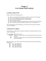
Total revenue

EXHIBIT 3.1
CVP Graph for Magik
Bicycles’ Magikbike III.
Breakeven point
$9,120,000
$8,800,000

$5,500,000

Total costs

Operating
income area

Dollars

ch03.qxd

Operating
loss area

11,000 11,400
Quantity of bikes

■ Breakeven Point
Q4 What is the breakeven

point?
CURRENT PRACTICE
The U.S. Small Business
Administration Web site
recommends the use of breakeven
analysis and refers small business
owners to a breakeven analysis
calculator and CVP graphing tool.2

Managers often want to know the level of activity required to break even. A CVP analysis
can be used to determine the breakeven point, or level of operating activity at which revenues cover all fixed and variable costs, resulting in zero profit. We can calculate the
breakeven point from any of the preceding CVP formulas, setting profit to zero. Depending
on which formula we use, we calculate the breakeven point in either number of units or in
total revenues. For Magikbike III, breakeven points are:
Breakeven quantity ϭ ($5,500,000 ϩ $0) Ϭ ($800 Ϫ $300) ϭ 11,000 bikes
Breakeven revenue ϭ ($5,500,000 ϩ $0) Ϭ 0.625 ϭ $8,800,000

■ Cost-Volume-Profit Graph
A cost-volume-profit graph (or CVP graph) shows the relationship between total revenues
and total costs; it illustrates how an organization’s profits are expected to change under different volumes of activity. Exhibit 3.1 presents a CVP graph for Magikbikes III. Notice that
when no bikes are sold, fixed costs are $5,500,000, resulting in a loss of $5,500,000. As sales
volume increases, the loss decreases by the contribution margin for each bike sold. The cost
and revenue lines intersect at the breakeven point of 11,000, which means zero loss and zero
profit. Then as sales increase beyond this breakeven point, we see an increase in profit, growing by the $500 contribution margin for each bike sold. Profits achieve the target level of
$200,000 when sales volume reaches 11,400.

GUIDE YOUR LEARNING 3.1 Key Terms
Stop to confirm that you understand the new terms introduced in the last several pages.
Cost-volume-profit (CVP) analysis (p. 89)
Contribution margin (p. 89)

Contribution margin per unit (p. 89)
Contribution margin ratio (CMR) (p. 90)

*Sales mix (p. 90)
Breakeven point (p. 91)
Cost-volume-profit graph (p. 91)

For each of these terms, write a definition in your own words. For the starred term, list at least
one example that is different from the ones given in this textbook.

2Do

a search for Breakeven Analysis at the U.S. Small Business Administration Web site, available at www.sba.gov.


ch03.qxd

9/27/04

4:06 PM

Page 92

To download more slides, ebook, solutions and test bank, visit

92

CHAPTER 3 ➤ COST-VOLUME-PROFIT ANALYSIS

■ CVP with Income Taxes

ALTERNATIVE TERMS
Some people use the terms operating
income (loss) or income (loss) before
income taxes instead of pretax profit
(loss). Similarly, some people use net
income (loss) instead of after-tax
profit (loss).

Up to this point, our CVP calculations ignored income taxes. An organization’s after-tax
profit is calculated by subtracting income tax from pretax profit. The tax is usually calculated as a percentage of pretax profit.
After-tax profit ϭ Pretax profit Ϫ Taxes
ϭ Pretax profit Ϫ (Tax rate ϫ Pretax profit)
ϭ Pretax profit ϫ (1 Ϫ Tax rate)

If we want to know the amount of pretax profit needed to achieve a target level of after-tax
profit, we solve the preceding formula for pretax profit:
After-tax profit
Pretax profit ϭ ᎏᎏ
(1 Ϫ Tax rate)

Suppose that Magik Bicycles plans for an after-tax profit of $20,000 and its tax rate is
30%. Then,
Pretax profit ϭ $20,000 Ϭ (1 Ϫ 0.30) ϭ $28,571

The company needs a pretax profit of $28,571 to earn an after-tax profit of $20,000.
The following illustration develops a cost function to calculate the volumes needed to
break even and to achieve a target after-tax profit when multiple products are involved.

DIE GEFLECKTE KUH EIS (THE SPOTTED COW CREAMERY) (PART 1)
CVP ANALYSIS WITH INCOME TAXES

Die Gefleckte Kuh Eis (The Spotted Cow Creamery) is a popular ice cream emporium near a university in Munich, Germany. Information for the most recent month (amounts in euros) appears here.
Revenue
Cost of food and beverages sold
Labor
Rent
Pretax profit
Income taxes (25%)
After-tax profit

40,000
20,000
15,000
1, 000
ᎏᎏᎏᎏᎏᎏᎏᎏ
4,000
1, 000
ᎏᎏᎏᎏᎏᎏᎏᎏ
3, 000
ᎏ
ᎏᎏᎏᎏ
ᎏᎏᎏᎏ
ᎏᎏ
ᎏᎏ
ᎏ
The store owner asked the manager, Holger Soderstrom, to estimate results for the next
month. This particular outlet has not performed as well as the owner’s other three outlets. Holger believes that sales volumes will increase to 48,000 next month because it has been an unusually hot and dry summer.

Estimating the Cost Function
To perform CVP analysis, Holger first estimates the cost function. Using accounting records, he classifies each cost as fixed or variable and then estimates next month’s cost. Of the costs listed in the
accounting records, labor ( 15,000) and rent ( 1,000) are most likely fixed (assuming employees

work fixed schedules). Assuming that fixed costs do not change from month to month, Holger’s best
estimate of next month’s fixed costs is 16,000 ( 15,000 ϩ 1,000). The remaining item, cost of
food and beverages sold ( 20,000), is most likely a variable cost. Because The Spotted Cow Creamery’s focus is retail sales of ice cream and other food items, Holger can reasonably assume that sales
volume drives this variable cost. Thus, he estimates expected variable costs as a percent of revenue:
20,000 Ϭ 40,000 ϭ 0.50, or 50% of revenue
Holger combines his fixed and variable cost estimates to create the following cost function for next month:
TC ϭ 16,000 ϩ (50% ϫ Revenues)

Estimating After-Tax Profit
If next month’s revenues are 48,000, Holger expects total variable costs to be (50% ϫ 48,000) ϭ
24,000. Therefore, his estimate of pretax profit is
Pretax profit ϭ 48,000 Ϫ 16,000 Ϫ 24,000 ϭ 8,000


ch03.qxd

9/27/04

4:06 PM

Page 93

To download more slides, ebook, solutions and test bank, visit

COST-VOLUME-PROFIT ANALYSIS

93

Holger estimates income taxes and after-tax profit, assuming that income taxes remain at 25% of
pretax profit:

After-tax profit ϭ 8,000(1 Ϫ 0.25) ϭ 6,000

Calculating Revenues to Achieve Targeted After-Tax Profit
Holger presents the preceding information to the owner. However, the owner still has concerns
about this outlet because the other outlets have achieved after-tax profits of about 8,000 each
during the last few months. The owner thinks that sales volume might be the problem. To help analyze this possibility, Holger determines the sales volume necessary to earn after-tax profits of 8,000
per month. He begins by calculating the targeted pretax profit:
Pretax profit ϭ 8,000 Ϭ (1 Ϫ 0.25) ϭ 10,667
Next, he uses the following CVP formula to solve for targeted revenue:
F ϩ Profit
Revenues ϭ ᎏᎏ
CMR
Substituting in the preceding information:
Revenues ϭ ( 16,000 ϩ 10,667) Ϭ 0.50 ϭ 53,334
Notice that Holger uses the contribution margin ratio calculated with the sales revenue and variable costs from his original analysis.
Holger summarizes his target profit calculations for the owner as follows:
Revenue
Cost of food and beverages sold (50% of
Labor (fixed)
Rent (fixed)
Pretax profit
Income taxes (25%)
After-tax profit

53,334
26,667
15,000
1, 000
ᎏᎏᎏᎏᎏᎏᎏᎏ
10,667

2, 667
ᎏᎏᎏᎏᎏᎏᎏᎏ
8, 000
ᎏ
ᎏᎏᎏᎏ
ᎏᎏᎏᎏ
ᎏᎏ
ᎏᎏ
ᎏ
8,000, revenues need to increase by 33%
53,334)

For the outlet to achieve an after-tax profit of
[( 53,334 Ϫ 40,000) Ϭ 40,000] over last month.
Holger presents this information to the owner and argues that sales will increase to 53,334
because the weather will be hotter next month. However, the owner thinks that Holger may be worried about being replaced, and so his revenue estimates are probably biased upwards. The owner
decides to investigate Holger’s estimates further by comparing his revenues and costs to those in
the other outlets.

GUIDE YOUR LEARNING 3.2 The Spotted Cow Creamery (Part 1)
The Spotted Cow Creamery (Part 1) illustrates a multiple-product CVP analysis with income taxes. For this illustration:

Define It

Identify Problem
and Information

Which definitions, analysis techniques, and
computations were
used?

What decisions were
being addressed? What
information was relevant to the decisions?

Identify Uncertainties

Explore Assumptions

Explore Biases

What types of uncertainties were there?
Consider uncertainties
about:
● Revenue and cost
estimates
● Interpreting results
● Relevant range of
operations
● Feasibility of activity
level

Reread the first part of
this chapter and identify the assumptions
used in developing the
CVP formulas. How
reasonable are these
assumptions for The
Spotted Cow Creamery?

Why and how might
the manager’s bias
influence the computations? Why would the
owner be uncertain
whether the manager
had created biased revenue or cost estimates?


ch03.qxd

9/27/04

4:06 PM

Page 94

To download more slides, ebook, solutions and test bank, visit

94

CHAPTER 3 ➤ COST-VOLUME-PROFIT ANALYSIS

PERFORMING CVP
ANALYSES WITH
A SPREADSHEET

Spreadsheets are often used for CVP computations, particularly when an organization
has multiple products. Spreadsheets simplify the basic computations and can be designed
to show how changes in volumes, selling prices, costs, or sales mix alter the results.

Q3 How are CVP

■ CVP Calculations for a Sales Mix

calculations performed
for multiple products?

Although The Spotted Cow Creamery sells multiple products, the CVP analysis performed
by the store manager did not provide computations for individual products. Instead, the analysis focused on the total amount of revenue needed to achieve a target profit. If the manager
wants to use CVP results to plan future operations for individual products, the required revenue for each product needs to be determined. Such computations are performed using the
sales mix. The sales mix should be stated as a proportion of units when performing CVP
computations in units, and it should be stated as a proportion of revenues when performing
CVP computations in revenues. Sales mix computations can become cumbersome if performed manually; it is easiest to use a spreadsheet.
To demonstrate CVP computations using a spreadsheet, suppose that Magik Bicycles
developed three different products, a small bike for children and youths, a road bike, and a
mountain bike. Total fixed costs for the company are $14,700,000. Forecasted sales volumes
are as follows. The sales mix in percentages is calculated from these volumes.
Forecasted volume (units)
Expected sales mix in units

Youth
10,000
25%

Road
18,000
45%

Mountain
12,000

30%

Total
40,000
100%

Because of increased competition and an economic downturn, the managers of Magik Bicycles are uncertain about the company’s ability to achieve the forecasted level of sales. They
would like to know the minimum amount of sales needed for an after-tax profit of $100,000.
The company’s income tax rate is 30%. The expected unit selling prices, variable costs, and
contribution margins for each product are as follows:
Price per unit
Variable cost per unit
Contribution margin per unit

CURRENT PRACTICE
Spreadsheet skills are important
professionally. The American
Institute of Certified Public
Accountants (AICPA) states that an
entry-level accountant should be
able to “appropriately use electronic
spreadsheets and other software to
build models and simulations.”3

Youth
$200
75
ᎏ ᎏᎏᎏ
$125
ᎏᎏ

ᎏᎏ
ᎏᎏ
ᎏ
ᎏ

Road
$700
250
ᎏᎏᎏᎏ
$450
ᎏᎏ
ᎏᎏ
ᎏᎏ
ᎏ
ᎏ

Mountain
$800
ᎏ3
ᎏ0
ᎏ0
ᎏ
$500
ᎏᎏ
ᎏᎏ
ᎏᎏ
ᎏ
ᎏ

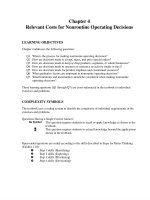
Exhibit 3.2 shows a sample CVP spreadsheet for Magik Bicycles. Notice that all of the

input data is placed in an area labeled as “Input section” in the spreadsheet. The calculations
are performed outside of this area (formulas for this spreadsheet are shown in Appendix 3A).
Spreadsheets designed this way allow users to alter the assumptions in the input section without performing any additional programming.
The spreadsheet in Exhibit 3.2 first uses the input data to compute expected revenues,
costs, and income. The revenues and variable costs for each product are computed by multiplying the expected sales volume times the selling price and variable cost per unit shown
in the input area. The revenues and variable costs for the three products are then combined
to determine total revenues and total variable costs for the company. After subtracting expected fixed costs and income taxes (30% of pretax income), the expected after-tax income
is $455,000.
When an organization produces and sells a number of different products or services, we
use the weighted average contribution margin per unit to determine the breakeven point or
target profit in units. Similarly, we use the weighted average contribution margin ratio to determine the breakeven point or target profit in revenues. “Weighted average” here refers to
the expected sales mix: 10,000 youth bikes or $2,000,000 in revenues, 18,000 road bikes or

3This

skill is an element of the competency “Leverage Technology to Develop and Enhance Functional Competencies,” AICPA Core Competency Framework, accessed through the Library at eca.aicpaservices.org/.


ch03.qxd

9/27/04

4:06 PM

Page 95

To download more slides, ebook, solutions and test bank, visit

PERFORMING CVP ANALYSES WITH A SPREADSHEET

EXHIBIT 3.2
Spreadsheet for Magik
Bicycles CVP with
Multiple Products

A
1
2
3
4
5
6
7
8
9
10
11
12
13
14
15
16
17
18
19
20
21
22
23
24

25
26
27
28
29
30
31
32
33
34
35
36
37
38
39
40
41
42
43
44
45
46
47
48
49
50
51
52

Input section

Expected sales volume-units
Price per unit
Variable cost per unit
Fixed costs
Desired after-tax profit
Income tax rate

Contribution Margin
Units
Revenue
Variable costs
Contribution margin
Contrib. margin per unit
Contrib. margin ratio
Expected sales mix in units
Expected sales mix in revenues

B
Youth Bikes
10,000
$200
$75

C
Road Bikes
18,000
$700
$250

D

95

E

Mtn. Bikes
12,000
$800
$300

$14,700,000
$100,000 (enter zero for breakeven)
30%

Youth Bikes
10,000
$2,000,000
750,000
$1,250,000

Road Bikes
18,000
$12,600,000
4,500,000
$8,100,000

Mtn. Bikes
12,000
$9,600,000
3,600,000

$6,000,000

Total Bikes
40,000
$24,200,000
8,850,000
$15,350,000

$125.00
62.50%

$450.00
64.29%

$500.00
62.50%

$383.75
63.43%

25.00%
8.26%

45.00%
52.07%

30.00%
39.67%

100.00%

100.00%

Expected Income
Contribution margin (above)
Fixed costs
Pretax income
Income taxes
After-tax income

$15,350,000
14,700,000
650,000
195,000
$455,000

Preliminary CVP Calculations
Target pretax profit for CVP analysis
Fixed costs plus target pretax profit

$142,857
$14,842,857

CVP analysis in units
CVP calculation in units
Revenue
Variable costs
Contribution margin
Fixed costs
Pretax income
Income taxes

After-tax income

Youth Bikes
9,669.614
$1,933,923
725,221
$1,208,702

Road Bikes
17,405.305
$12,183,713
4,351,326
$7,832,387

Mtn. Bikes
11,603.537
$9,282,829
3,481,061
$5,801,768

Total Bikes
38,678
$23,400,465
8,557,608
14,842,857
14,700,000
142,857
42,857
$100,000

CVP analysis in revenues
CVP calculation in revenues
Variable costs
Contribution margin
Fixed costs
Pretax income
Income taxes
After-tax income

Youth Bikes
$1,933,923
725,221
$1,208,702

Road Bikes
$12,183,713
4,351,326
$7,832,387

Mtn. Bikes
$9,282,829
3,481,061
$5,801,768

Total Bikes
$23,400,465
8,557,608
14,842,857
14,700,000
142,857

42,857
$100,000

Note: Appendix 3A provides a version of this spreadsheet showing the cell formulas.

$12,600,000 in revenues, and 12,000 mountain bikes or $9,600,000 in revenues. Given the
sales mix, the weighted average contribution margin per unit is calculated as the combined
contribution margin ($15,350,000) divided by the total number of units expected to be sold
(40,000), or $383.75 per unit as computed in Exhibit 3.2.4 The weighted average contribution margin ratio is the combined contribution margin ($15,350,000) divided by combined
revenue ($24,200,000), or 63.43%.5
4Another

way to compute the weighted average contribution margin per unit is to sum the contribution margins for
the three products, weighted by number of units sold as follows: (10,000 Ϭ 40,000)($200 Ϫ $75) ϩ (18,000 Ϭ
40,000)($700 Ϫ $250) ϩ (12,000 Ϭ 40,000)($800 Ϫ $300) ϭ $383.75.
5Another way to compute the weighted average contribution margin ratio is to sum the contribution margin ratios for the
three products, weighted by revenues as follows: ($2,000,000 Ϭ $24,200,000)[($200 Ϫ $75) Ϭ $200] ϩ ($12,600,000 Ϭ
$24,200,000)[($700 Ϫ $250) Ϭ $700] ϩ ($9,600,000 Ϭ $24,200,000)[($800 Ϫ $300) Ϭ $800] ϭ 63.43%.


ch03.qxd

9/27/04

4:06 PM

Page 96

To download more slides, ebook, solutions and test bank, visit

96

CHAPTER 3 ➤ COST-VOLUME-PROFIT ANALYSIS

The spreadsheet in Exhibit 3.2 performs CVP computations using both units and revenues. To achieve an after-tax target profit of 100,000, the company must earn a pretax profit
of $142,857 [$100,000 Ϭ (1 Ϫ 0.30)]. To compute the total number of units (bikes) that must
be sold to achieve the target profit, we divide the fixed costs plus the target profit by the
weighted average contribution margin per unit:
$14,700,000 ϩ $142,857
F ϩ Profit
Units needed for target profit ϭ Q ϭ ᎏᎏ ϭ ᎏᎏᎏ ϭ 38,678 units
(P Ϫ V )
$383.75 per unit

Magik needs to sell 38,678 units to achieve an after-tax target profit of $100,000. To determine the number of units for each product that must be sold, we multiply the total number
of units (38,678) by each product’s expected sales mix in units. For example, the company
must sell 38,678 units ϫ (10,000 units Ϭ 40,000 units), or 9,670 youth bikes.
To calculate the amount of revenue needed to achieve the target after-tax profit of
$100,000, we divide the fixed costs plus the target pretax profit by the weighted average
contribution margin ratio:
F ϩ Profit
$14,700,000 ϩ $142,857
Revenues ϭ ᎏᎏ ϭ ᎏᎏᎏ ϭ $23,400,373
CMR
63.43%

The difference between the spreadsheet and this hand-calculated amount is due to rounding, as are any differences in the following amounts. To determine the revenues for each
product that must be sold, we multiply the total revenues ($23,400,373) by each product’s
expected sales mix in revenues. For example, the company must achieve $23,400,373 ϫ
($2,000,000 Ϭ $24,200,000), or $1,933,914 in revenues from youth bikes. Notice that the

required revenue for each product is equal to the required number of units times the expected selling price. For youth bikes, 9,670 units ϫ $200 per unit ϭ $1,934,000.
The results of calculations using units and revenues are always identical. Because information in the example was given in units, it would have been easiest to create the spreadsheet using only the computations for CVP in units. However, in some situations per-unit
information is not available. In those cases, it is necessary to perform CVP calculations using revenues. Later in the chapter we revisit the ice cream shop illustration to analyze the
influence of sales mix on the total contribution margin.

■ CVP Sensitivity Analysis
Q5 What assumptions and
limitations should
managers consider
when using CVP
analysis?

One of the benefits of creating a spreadsheet with a separate input section is that additional
CVP analyses can easily be performed by the changing input data. For example, suppose the
managers of Magik Bicycles want to know the number of bikes they must sell to break even.
We can return to the spreadsheet in Exhibit 3.2 and change the “Desired after-tax profit”
to zero. The resulting spreadsheet, showing only CVP calculations in units, is presented in
Exhibit 3.3.
The managers of Magik Bicycles could use the CVP spreadsheet to perform several different types of sensitivity analyses. Suppose sales of the mountain bike are falling behind

EXHIBIT 3.3
Spreadsheet Results for
Magik Bicycles Breakeven
Analysis

31
32
33
34
35

36
37
38
39
40
41
42
43

A
Preliminary CVP Calculations
Target pretax profit for CVP analysis
Fixed costs plus target pretax profit
CVP analysis in units
CVP calculation in units
Revenue
Variable costs
Contribution margin
Fixed costs
Pretax income
Income taxes
After-tax income

B

C

D

E

$0
$14,700,000

Youth Bikes
9,576.547
$1,915,309
718,241
$1,197,068

Road Bikes
17,237.785
$12,066,450
4,309,446
$7,757,003

Mtn. Bikes
11,491.857
$9,193,485
3,447,557
$5,745,928

Total Bikes
38,306
$23,175,244
8,475,244
14,700,000
14,700,000
0
0
$0

ch03.qxd

9/27/04

4:06 PM

Page 97

To download more slides, ebook, solutions and test bank, visit

PERFORMING CVP ANALYSES WITH A SPREADSHEET

97

expectations. They could determine the effects of the change in sales mix on results. Every
assumption in the data input box is easily changed to update information. Sensitivity analysis helps managers explore the potential impact of variations in data they consider to be particularly important or uncertain.

■ Discretionary Expenditure Decision
Q1 What is cost-volumeprofit (CVP) analysis,
and how is it used for
decision making?

CHAPTER REFERENCE
Chapter 4 uses CVP analysis for
additional types of decisions. We
also learn that decisions are often
influenced by qualitative information
that is not valued in numerical terms.

CVP analysis also helps managers make business decisions such as whether to increase
or decrease discretionary expenditures. For example, suppose the managers of Magik
Bicycles want to advertise one of their products more heavily. A distributor pointed
out that the road bike price was less than a competitor’s price for a model with fewer
features. The competitor’s brand name is quite well known, but the distributor thinks
that he could sell at least 10% more road bikes if Magik launched a regional advertising campaign.
The managers of Magik estimate that an additional expenditure of $100,000 in advertising will increase road bike sales by 5%, to 18,900 bikes. To estimate the effects of the
proposed expenditure, we return to the spreadsheet in Exhibit 3.2 and make two changes.
First, fixed costs would increase by $100,000 to $14,800,000. Second, the expected volume
of road bikes sold would increase to 18,900. The resulting spreadsheet in Exhibit 3.4 indicates that after-tax profits are expected to increase by $213,500 from $455,000 to $668,500.
Notice on the spreadsheet that the change in sales mix affects the weighted average contribution margin; it changes from 383.75 to $385.21.
We could perform the same calculation without the spreadsheet by subtracting the
$100,000 investment in fixed costs from the additional contribution margin of $405,000
[900 bikes ϫ ($700 Ϫ $250)]. The resulting incremental after-tax profit is $213,500
[($405,000 Ϫ $100,000)(1 Ϫ 0.30)]. Because profits are expected to increase more than
costs for this advertising campaign, the managers would be likely to make the additional
investment.

■ Planning, Monitoring, and Motivating with CVP

CHAPTER REFERENCE
In Chapter 10, CVP analysis is used to
create flexible budgets for measuring
and monitoring performance at
different levels of activity.

CVP analyses are useful for planning and monitoring operations and for motivating employee
performance. If the owner of The Spotted Cow Creamery obtains similar information for the
other outlets, results can be compared to identify differences in revenue levels and cost functions. For example, unusually high labor costs might suggest that the low-profit outlet is

overstaffed or inefficient. Once the owner analyzes the reasons for differences in profitability, emphasis can be placed on increasing revenues, reducing costs, or both. The owner can
also hold managers more accountable for performance, which should motivate their work efforts toward the owner’s goals.

EXHIBIT 3.4
Spreadsheet for Magik
Bicycles Advertising
Expenditure Decision

12
13
14
15
16
17
18
19
20
21
22
23
24
25
26
27
28
29

A
Contribution Margin
Units

Revenue
Variable costs
Contribution margin
Contrib. margin per unit
Contrib. margin ratio
Expected sales mix in units
Expected sales mix in revenues
Expected Income
Contribution margin (above)
Fixed costs
Pretax income
Income taxes
After-tax income

B
Youth Bikes
10,000
$2,000,000
750,000
$1,250,000

C
Road Bikes
18,900
$13,230,000
4,725,000
$8,505,000

D
Mtn. Bikes

12,000
$9,600,000
3,600,000
$6,000,000

E
Total Bikes
40,900
$24,830,000
9,075,000
$15,755,000

$125.00
62.50%

$450.00
64.29%

$500.00
62.50%

$385.21
63.45%

24.45%
8.05%

46.21%
53.28%

29.34%
38.66%

100.00%
100.00%

$15,755,000
14,800,000
955,000
286,500
$668,500


ch03.qxd

9/27/04

4:06 PM

Page 98

To download more slides, ebook, solutions and test bank, visit

98

CHAPTER 3 ➤ COST-VOLUME-PROFIT ANALYSIS

DIE GEFLECKTE KUH EIS (THE SPOTTED COW CREAMERY) (PART 2)
THE INFLUENCE OF SALES MIX ON PROFITABILITY
The owner of The Spotted Cow Creamery has several profitable stores. He asked the store managers to provide information about their sales mix, specifically the amount of beverage versus

ice cream products sold. Beverages provide a much larger contribution margin than ice cream.
After analyzing the data, he found that about half of the revenues in the most profitable stores
were for the sale of beverages. In addition, these stores have more stable sales throughout the
winter because they sell specialty coffee beverages as well as soft drinks.
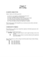
The owner shared this information with Holger, the manager of a less profitable store. Holger investigates the contribution margins from beverages and ice cream at his store. He sets up
a spreadsheet to examine the influence of the sales mix on profitability, shown in Exhibit 3.5(a).
He finds that beverages are about 15% of total revenue ( 6,000 Ϭ 40,000). The contribution
margin ratio for beverages is 93% ( 5,600 Ϭ 6,000), whereas the contribution margin for ice
cream is 42% ( 14,400 Ϭ 34,000). When he changes the desired sales mix in the spreadsheet
from 15% to 50% beverages to match the sales mix of more profitable stores, the after-tax income increases by a sizeable amount from 3,000 to 8,353 as indicated in Exhibit 3.5(b).
Holger realizes that several strategies would increase the percentage of beverages in his
current sales mix. First, he could require the sales clerks to suggest a beverage with each sale. In
addition, he could emphasize beverages in his advertising. He could also analyze his competitors’
beverage prices to be certain that his prices are competitive. A small drop in the price of beverages
might increase the volume of beverages sold more than enough to offset the decline in contribution margin ratio. He uses the spreadsheet to perform sensitivity analysis around these factors.

EXHIBIT 3.5 Spreadsheet for The Spotted Cow Creamery
A
1
2
3
4
5
6
7
8
9
10
11
12

13
14
15
16
17
18
19
20
21
22

B

C

A

D

Input section
Revenue
Variable cost
Current sales mix in revenues
Fixed costs
Tax rate
Desired sales mix in revenues

Contribution margin ratio
Income statement
Revenue

Variable cost
Contribution margin

Beverage
€6,000
400
15%

Ice Cream
€34,000
19,600
85%

15%

85%

Total
€40,000
20,000
100%
16,000
25%
100%

93%

42%

Weighted Average

50%

€6,000
400
5,600

€34,000
19,600
14,400

€40,000
20,000
20,000

Fixed costs
Pretax income
Taxes
After tax income

16,000
4,000
1,000
€3,000

(a) Current Sales Mix

1
2
3
4

5
6
7
8
9
10
11
12
13
14
15
16
17
18
19
20
21
22

B

C

D

Input section
Revenue
Variable cost
Current sales mix in revenues
Fixed costs

Tax rate
Desired sales mix in revenues

Contribution margin ratio
Income statement
Revenue
Variable cost
Contribution margin

Beverage
€6,000
400
15%

Ice Cream
€34,000
19,600
85%

50%

50%

Total
€40,000
20,000
100%
16,000
25%
100%

93%

42%

Weighted Average
68%

€20,000
1,333
18,667

€20,000
11,529
8,471

€40,000
12,863
27,137

Fixed costs
Pretax income
Taxes
After tax income

16,000
11,137
2,784
€8,353

(b) Desired Sales Mix

GUIDE YOUR LEARNING 3.3 The Spotted Cow Creamery (Part 2)
The Spotted Cow Creamery (Part 2) illustrates the influence of sales mix on profitability. For this
illustration:
Compute It

Identify Uncertainties

Explore Uses

For Exhibit 3.5, manually
recalculate:
● Sales mix in units
● Sales mix in revenues
● Weighted average contribution margin ratio

At the end of the illustration,
the store manager was considering several strategies for
changing his store’s sales mix.
What uncertainties does the
manager face?

How was CVP information
used by the owner? How was
it used by the manager?


ch03.qxd

9/27/04

4:06 PM

Page 99

To download more slides, ebook, solutions and test bank, visit

ASSUMPTIONS AND LIMITATIONS OF COST-VOLUME-PROFIT ANALYSIS

ASSUMPTIONS AND
LIMITATIONS OF
COST-VOLUMEPROFIT ANALYSIS

99

Exhibit 3.6 summarizes the input data, assumptions, and uses of CVP analysis. CVP analysis relies on several assumptions. In Chapter 2 we assumed for the linear cost function
(F ϩ V ϫ Q) that production volumes are within a relevant range of operations where
fixed costs remain fixed and variable costs remain constant. In addition, for CVP analysis,
we assume that selling prices remain constant and that the sales mix is constant. Sensitivity
analysis can be performed to determine the sensitivity of profits to these assumptions.

Q5 What assumptions and
limitations should
managers consider
when using CVP
analysis?
CHAPTER REFERENCE
Chapter 2 explains the importance of
the relevant range in measuring the

cost function.

■ Uncertainties and Quality of Input Data
As indicated in Exhibit 3.6, CVP analysis relies on forecasts of expected revenues and
costs. CVP assumptions rule out fluctuations in revenues or costs that might be caused by
common business factors such as supplier volume discounts, learning curves, changes in production efficiency, or special customer discounts. In addition, many uncertainties may arise
about whether CVP assumptions will be violated, such as the following:
●
●
●
●

●
●

Can volume of operating activity be achieved?
Will selling prices increase or decrease?
Will sales mix remain constant?
Will fixed or variable costs change as operations move into a new relevant
range?
Will costs change due to unforeseen causes?
Are revenue and cost estimates biased?

EXHIBIT 3.6 Input Data, Assumptions, and Uses of CVP Analysis
Use Results to:
Describe volume, revenues, costs, and profits:
●

Values at breakeven or target profit.:
–Units sold

–Revenues
–Variable, fixed, and total costs

●

Sensitivity of results to changes in:
–Levels of activity
–Selling price
–Cost function
–Sales mix

●

Indifference point between alternatives
Feasibility of planned operations

CVP Analysis and Assumptions
Calculate number of units or revenues needed for:

Input Data for
CVP Analysis
Expected Revenues
(volume and selling
price)
Expected Costs
(cost function)
Sales Mix (for multiple
products)

●

●

Breakeven
Target profit

Assumptions:

●

Operations within a relevant
range
● Linear cost function
–Fixed costs remain constant
–Variable cost per unit remains
constant
● Linear revenue function
–Sales mix remains constant
–Prices remain constant

Assist with plans and decisions such as:

●

●
●
●
●
●
●
●

●

Budgets
Product emphasis
Selling price
Production or activity levels
Employee work schedules
Raw material purchases
Discretionary expenditures such as advertising
Proportions of fixed versus variable costs

Monitor operations by comparing expected and
actual:
●
●

Volumes, revenues, costs, and profits
Profitability risk


ch03.qxd

9/27/04

4:06 PM

Page 100

To download more slides, ebook, solutions and test bank, visit

100

CHAPTER 3 ➤ COST-VOLUME-PROFIT ANALYSIS

EXHIBIT 3.7 Examples of Business Uncertainties
Ashanti
Goldfields
Company Ltd.

Coca-Cola
FEMSA,
S.A. de C.V.

Bank of
Montreal

Nokia
Corporation

eBay, Inc.

Sony
Corporation

Ghana

Canada

Mexico

United States

Finland

Japan

Gold mining and
exploration

Credit and noncredit banking
services

Production and
distribution of
Coca-Cola
products

Web-based marketplace and payment services

Mobile communications

Electronic equipment design and
manufacturing

Gold prices
Anticipated life
of mines
● Power supply
● Labor relations

●

Changes in
global capital
markets
● Interest rates
● Regulatory
changes
● Technological
changes

●

Deterioration in
relationships with
the Coca-Cola
Company
● Governmental
price controls
● More stringent
environmental
regulations
● High inflation

●

Retaining active
user base
● Consumer confidence in Web site
security

● Management of
fraud loss
● Retaining key
employees

●

Global network
reliance on large
multiyear contracts
● Failure of product quality
● System or network disruptions
● Electromagnetic
field-related
litigation

●

Examples adapted from
“Forward-Looking Information” in Form
20-F (filed with the
SEC).

Examples adapted from
“Caution Regarding
Forward-Looking
Statements” under
“Investor Relations” at
www4.bmo.com.

Examples adapted from
“Cautionary Statements”
in presentation to J.P.
Morgan, July 2003

Examples adapted from
“Risk Factors That May
Affect Results of Operations and Financial
Condition” in 2002
annual report.

Examples adapted from
“Risk Factors” in 2002
annual report.

Examples adapted from
“Cautionary Statement”
under Investor Relations at www.sony.net/
index.html.

●
●

CHAPTER REFERENCE
We address the quality of expected
revenue and cost information further
in Chapter 10 (budgeting).

Levels of consumer spending
● Speed and nature of technology

change
● Change in consumer preferences
● Ability to reduce
workforce

All organizations are subject to uncertainties, leading to risk that they will fail to meet
expectations. Exhibit 3.7 summarizes major business uncertainties for six companies in a variety of industries around the world. Even though each organization is subject to unique business risks, all face uncertainties related to the economic environment. Some organizations are
subject to more uncertainty than others. For example, uncertainties are greater in industries
experiencing rapid technological and market change or intense competition.

■ Quality of CVP Technique
To help managers make better decisions, accountants evaluate the quality of the techniques they
use, given the organizational setting and decisions to be made. This evaluation helps determine
when techniques such as CVP analysis are likely to be an appropriate tool and how much reliance to place on the results. The quality of information generated from an analysis technique
is higher if the economic setting is consistent with the technique’s underlying assumptions.
Strict CVP assumptions are violated in many business settings. The types of uncertainties already discussed can lead to nonlinear behavior in revenues and costs. In addition, it
may be difficult to determine the point of operating activity where operations move into a
new relevant range.
Nevertheless, in many business settings CVP analysis provides useful information. Accountants and managers use their knowledge of the organization’s operations and their judgment to evaluate whether the CVP assumptions are reasonable for their setting. They can
rely more on CVP results when the assumptions are less likely to be violated. Also, the data
used in CVP calculations must be updated continually to be useful.

■ CVP for Nonprofit Organizations
The basic CVP formulas in this chapter are written for typical for-profit businesses such as
manufacturers, retailers, or service providers. Nonprofit organizations often receive grants
and donations. These revenue sources complicate CVP calculations because they could be
affected by quantity of goods or services sold. Grants and donations that are unrelated to the


ch03.qxd

9/27/04

4:06 PM

Page 101

To download more slides, ebook, solutions and test bank, visit

ASSUMPTIONS AND LIMITATIONS OF COST-VOLUME-PROFIT ANALYSIS

101

quantity of goods or services sold are offset against fixed costs in the CVP formulas. However, when grants and donations vary with a not-for-profit organization’s operating activities, they might be included in revenues or subtracted from variable costs. The treatment depends on the nature of the grant or donation.
The following illustration continues the story of Small Animal Clinic from Chapter 2.
Recall that Small Animal Clinic is a not-for-profit organization that treats small animals. It
received a foundation grant that matches incoming revenues. For example, if a pet owner
pays $30 in fees, the foundation matches with an additional $30 to the clinic. In this case,
the grant is included in revenues for CVP calculations.

SMALL ANIMAL CLINIC
NOT-FOR-PROFIT ORGANIZATION CVP ANALYSIS
WITH TWO RELEVANT RANGES
Leticia Brown, Small Animal Clinic manager, and the accountant, Josh Hardy, are completing the
operating budget for 2006. Leticia estimated that the clinic will experience 3,800 animal visits,
and Josh estimated the cost function as follows:6
TC ϭ $119,009 ϩ $16.40Q
where Q is the number of animal visits. Leticia and Josh budgeted revenue per animal visit at
$60 ($30 in fees plus $30 in matching grant). Thus, they estimated that the clinic should achieve
a surplus of $46,671[($60)(3,800) Ϫ $119,009 Ϫ ($16.40)(3,800)]. The clinic is a not-for-profit

organization and pays no income taxes on its surplus.
To complete the planning process for next year, Leticia asks Josh to compute the clinic’s
breakeven point. As manager of a not-for-profit organization, she is particularly sensitive to financial risk and wants to know how much the clinic’s activity levels could drop before a loss would
occur.

Breakeven Compared to Budget
Josh performs the following calculations. With revenue per visit of $60, the contribution margin
per animal visit is
P Ϫ V ϭ $60.00 Ϫ $16.40 ϭ $43.60
Josh solves for Q with profit equal to $0 to find the breakeven point in number of animal visits:
($119,009 ϩ $0)
F ϩ Profit
Q ϭ ᎏᎏ ϭ ᎏᎏ ϭ 2,730 visits
(P Ϫ V )
$43.60
Leticia is pleased to see that the budgeted number of animal visits (3,800) is significantly
higher than the breakeven number. This result gives her considerable assurance that the clinic is
not likely to incur a loss, even if revenues fail to achieve targeted levels or if costs exceed estimated amounts.

Potential Investment in New Equipment
During the first two months of 2006, Leticia learns that the number of animal visits at Small Animal Clinic is running approximately 10% higher than the budget, and costs seem to be under control. Leticia thinks that the clinic might be on track for a high surplus this year.
For the past two years, Leticia has been interested in purchasing equipment costing $200,000
to provide low-cost neutering services. This year PAWS, a local charity, offered to pay for half of
the equipment cost, but only after the clinic raises the other half of the funds. Currently the clinic
has no excess cash because surpluses from prior years were invested in other projects. Thus, the
(continued)
the Chapter 2 illustration Small Animal Clinic (Part 2), the cost function was calculated as: TC ϭ $119,009 ϩ
($15.20)(Number of animal visits) ϩ (0.04)(Fee revenue). If average fee revenue is $30 per animal visit, then
the last term in the cost function can be rewritten as (0.04)($30)(Number of animal visits), which can be
simplified as ($1.20)(Number of animal visits). This substitution allows the cost function to be rewritten as:

TC ϭ $119,009 ϩ ($16.40)(Number of animal visits). This version of the cost function is appropriate for estimating total costs for the clinic, but it would not be appropriate for estimating total costs for a single animal visit, where the fees vary depending on the services performed.

6 In


ch03.qxd

9/27/04

4:06 PM

Page 102

To download more slides, ebook, solutions and test bank, visit

102

CHAPTER 3 ➤ COST-VOLUME-PROFIT ANALYSIS
clinic needs to raise $100,000 to receive the PAWS grant. Leticia asks Josh to calculate the number
of animal visits needed to achieve a surplus of $100,000.

Calculating and Analyzing Targeted Activity Level
Josh calculates the expected quantity needed to achieve $100,000 surplus as follows:
$119,009 ϩ $100,000
F ϩ Profit
$219,009
Q ϭ ᎏᎏ ϭ ᎏᎏᎏ ϭ ᎏ ϭ 5,024 animal visits
PϪV
$60.00 Ϫ $16.40
$43.60

He then calculates the total dollar amount of revenue needed:
$119,009 ϩ $100,000
F ϩ Profit
Revenues ϭ ᎏᎏ ϭ ᎏᎏᎏ ϭ $310,389
(P Ϫ V )/P
$43.60/$60.00
Josh tells Leticia that the clinic will need to earn $301,389 in revenues or 5,024 visits to achieve a
surplus of $100,000.
The budgeted level of activity (3,800 animal visits) is substantially higher than the level of activity needed to break even (2,730 animal visits). If animal visits continue to exceed this year’s budget
by 10%, Josh estimates that animal visits will reach 4,180 (3,800 ϫ 1.10) by year-end. However,
he thinks that it would be very difficult to achieve a targeted surplus of $100,000 (5,024 animal
visits).

CVP Adjusted for Change in Relevant Range
As Josh works on his report, he realizes that the clinic’s cost function might change if the number of animal visits gets very high. Leticia told him that she will probably hire another technician
and need to rent more space and purchase additional equipment if animal visits exceed 4,000 this
year. Therefore, Josh’s cost function for 5,024 visits is wrong. He develops a new cost function assuming that an additional technician, space, and equipment will increase fixed costs by about
$60,000 per year.
TC ϭ ($119,009 ϩ $60,000) ϩ $16.40Q ϭ $179,009 ϩ $16.40Q, for Q Ͼ 4,000
Thus, Josh’s earlier CVP analysis was incorrect when animal visits exceed 4,000. The level of activity needed for a targeted surplus of $100,000 needs to be recalculated:
($179,009 ϩ $100,000) Ϭ $43.60 ϭ 6,400 for Q Ͼ 4,000
Josh notices that an activity level of 6,400 animal visits is noticeably higher than the 5,024 visits
he first calculated. He realizes how important it is to adjust for the relevant range when performing CVP analyses.
When Josh shows Leticia the new results, they agree that the clinic cannot raise the funds for
new equipment by increasing the number of visits to 6,400. Leticia may need to cut costs or seek
other ways to pay for the neutering equipment. The additional fixed cost would also require the
clinic to have a much higher volume of operations to avoid a loss.

GUIDE YOUR LEARNING 3.4 Small Animal Clinic
Small Animal Clinic illustrates a CVP analysis with target profit and two relevant ranges for a not-for-profit organization. For this

illustration:

Define It

Identify Problem
and Information

Describe how the CVP computations change when more
than one relevant range is
involved.

What decisions were being
addressed? Why was CVP
information useful for the
decisions?

Identify Uncertainties

Explore Assumptions

What were the uncertainties?
Consider uncertainties about:
● Revenue and cost estimates
● Interpreting results
● Relevant range of operations
● Feasibility of activity level

How reasonable are the CVP
assumptions for Small Animal
Clinic?

9/27/04

4:06 PM

Page 103

To download more slides, ebook, solutions and test bank, visit

MARGIN OF SAFETY AND DEGREE OF OPERATING LEVERAGE

103

MARGIN OF SAFETY
AND DEGREE
OF OPERATING
LEVERAGE

In Small Animal Clinic, the manager used CVP information to help her learn how much
the volume of business could decline before the clinic would incur a loss. The manager
of Spotted Cow Creamery was able to identify the specific products to emphasize for
increased profitability. Managers are often interested in these types of questions. In addition, information from CVP analysis can be used to help manage operational risk.

Q6 How are margin of

■ Margin of Safety

safety and operating
leverage used to assess

operational risk?

The margin of safety is the excess of an organization’s expected future sales (in either revenue or units) above the breakeven point. The margin of safety indicates the amount by which
sales could drop before profits reach the breakeven point:
Margin of safety in units ϭ Actual or estimated units of activity Ϫ Units at breakeven point
Margin of safety in revenues ϭ Actual or estimated revenue Ϫ Revenue at breakeven point

The margin of safety is computed using actual or estimated sales values, depending on the
purpose. To evaluate future risk when planning, use estimated sales. To evaluate actual risk
when monitoring operations, use actual sales. If the margin of safety is small, managers may
put more emphasis on reducing costs and increasing sales to avoid potential losses. A larger
margin of safety gives managers greater confidence in making plans such as incurring additional fixed costs.
The margin of safety percentage is the margin of safety divided by actual or estimated
sales, in either units or revenues. This percentage indicates the extent to which sales can decline before profits become zero.
Margin of safety in units
Margin of safety percentage in units ϭ ᎏᎏᎏ
Actual or estimated units
Margin of safety in revenue
Margin of safety percentage in revenues ϭ ᎏᎏᎏ
Actual or estimated revenue

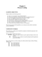
When the original budget was created for Small Animal Clinic, the breakeven point
was calculated as 2,730 animal visits, or $163,800 in revenues. However, Leticia and
Josh expected 3,800 animal visits, for $228,000 in revenue. Their margin of safety
in units of animal visits was 1,070 (3,800 Ϫ 2,730) and in revenues was $64,200
($228,000 Ϫ $163,800). Their margin of safety percentage was 28.2% (1,070 Ϭ 3,800,
or $64,200 Ϭ $228,000). In other words, their sales volume could drop 28.2% from expected levels before they expected to incur a loss. Exhibit 3.8 provides a CVP graph for
this information.

EXHIBIT 3.8

CVP Graph and Margin of
Safety for Small Animal
Clinic

Total Revenue
Estimated
Surplus = $64,200
Total Costs

$228,000
Dollars

ch03.qxd

Margin of Safety in
Revenues = $64,200

$163,800

Margin of Safety = 1,070 visits
Breakeven Point =
2,730 animal visits

Expected visits =
3,800 visits
Quantity of Animal Visits


ch03.qxd

9/27/04

4:06 PM

Page 104

To download more slides, ebook, solutions and test bank, visit

104

CHAPTER 3 ➤ COST-VOLUME-PROFIT ANALYSIS

■ Degree of Operating Leverage
Managers decide how to structure the cost function for their organizations. Often, potential
trade-offs are made between fixed and variable costs. For example, a company could purchase
a vehicle (a fixed cost) or it could lease a vehicle under a contract that charges a rate per
mile driven (a variable cost). Exhibit 3.9 lists some of the common advantages and disadvantages of fixed costs. One of the major disadvantages of fixed costs is that they may be
difficult to reduce quickly if activity levels fail to meet expectations, thereby increasing the
organization’s risk of incurring losses.
The degree of operating leverage is the extent to which the cost function is made up
of fixed costs. Organizations with high operating leverage incur more risk of loss when sales
decline. Conversely, when operating leverage is high an increase in sales (once fixed costs
are covered) contributes quickly to profit. The formula for operating leverage can be written in terms of either contribution margin or fixed costs, as shown here.7
Contribution margin
Degree of operating leverage in terms
TR Ϫ TVC
(P Ϫ V ) ϫ Q
ϭ ᎏᎏᎏ ϭ ᎏ ϭ ᎏᎏ
of contribution margin
Profit

Profit
Profit
F
Degree of operating leverage in terms of fixed costs ϭ ᎏ ϩ 1
Profit

Managers use the degree of operating leverage to gauge the risk associated with their cost
function and to explicitly calculate the sensitivity of profits to changes in sales (units or
revenues):
% change in profit ϭ % change in sales ϫ Degree of operating leverage

For Small Animal Clinic, the variable cost per animal visit was $16.40 and the fixed costs
were $119,009. With budgeted animal visits of 3,800, the managers expected to earn a profit
of $46,671. The expected degree of operating leverage using the contribution margin formula is then calculated as follows:
($60 Ϫ $16.40) ϫ 3,800 visits
$165,680
Degree of operating leverage ϭ ᎏᎏᎏᎏ ϭ ᎏ ϭ 3.55
$46,671
$46,671

We arrive at the same answer of 3.55 if we use the fixed cost formula:
$119,009
Degree of operating leverage ϭ ᎏ ϩ 1 ϭ 2.55 ϩ 1 ϭ 3.55
$46,671

EXHIBIT 3.9
Advantages and
Disadvantages of
Fixed Costs

Common Advantages

Common Disadvantages

Fixed costs might cost less in total than
variable costs.
● Companies might require unique assets
(e.g., expert labor or specialized production
facilities) that must be acquired through longterm commitments.
● Fixed assets such as automation and robotics
equipment can significantly improve operating
efficiency.
● Fixed costs are easier to plan; they do not
fluctuate with levels of activity.

Investing in fixed resources might divert
management attention away from the
organization’s core competencies.
● Fixed costs typically require a longer
financial commitment; it can be difficult to
reduce them quickly.
● Underinvestment or overinvestment in fixed
costs could affect profits and may not easily
be changed in the short term.

●

●

see the relationship between the two formulas, recall the profit equation: Profit ϭ (P Ϫ V ) ϫ Q Ϫ F, which

can be rewritten as F ϩ Profit ϭ Contribution margin. In turn, Degree of operating leverage ϭ Contribution
margin Ϭ Profit ϭ (F ϩ Profit) Ϭ Profit ϭ (F Ϭ Profit) ϩ 1.

7To


ch03.qxd

9/27/04

4:06 PM

Page 105

To download more slides, ebook, solutions and test bank, visit

MARGIN OF SAFETY AND DEGREE OF OPERATING LEVERAGE

105

The degree of operating leverage and margin of safety percentage are reciprocals.
1
Margin of safety percentage ϭ ᎏᎏᎏᎏ
Degree of operating leverage
1
Degree of operating leverage ϭ ᎏᎏᎏ
Margin of safety percentage

If the margin of safety percentage is small, then the degree of operating leverage is large. In
addition, the margin of safety percentage is smaller as the fixed cost portion of total cost gets

larger. As the level of operating activity increases above the breakeven point, the margin of
safety increases and the degree of operating leverage decreases. For Small Animal Clinic,
the reciprocal of the margin of safety percentage is 3.55 (1 Ϭ 0.282). The reciprocal of the
degree of operating leverage is 0.282 (1 Ϭ 3.55).

■ Using the Degree of Operating Leverage to Plan
and Monitor Operations
CURRENT PRACTICE
Before 1983, Medicare used costbased payment. Hospitals had high
operating leverage because risk
of loss was low. After Medicare
changed to a flat fee per patient,
managers lowered their operating
leverage.8

Managers need to consider the degree of operating leverage when they decide whether to incur additional fixed costs, such as purchasing new equipment or hiring new employees. They
also need to consider the degree of operating leverage for potential new products and services that could increase an organization’s fixed costs relative to variable costs. If additional
fixed costs cause the degree of operating leverage to reach what they consider an unacceptably high level, managers often use variable costs—such as temporary labor—rather than
additional fixed costs to meet their operating needs.
For example, the technicians at the Small Animal Clinic are paid a salary and work
40-hour weeks. Suppose Leticia could hire part-time technicians at $20.00 per hour instead
of hiring full-time technicians at the current salaries of $78,009. If each visit requires about
an hour of technician time, the new cost function would be TC ϭ ($119,009 Ϫ $78,009) ϩ
($16.40 ϩ $20.00)Q ϭ $41,000 ϩ $36.40Q. The breakeven point decreases considerably to
1,738 animal visits [$41,000 Ϭ ($60.00 Ϫ $36.40) per animal visit] or $104,280. Profit at
Q ϭ 3,800 animal visits is $48,680 [$228,000 Ϫ $41,000 Ϫ (3,800 animal visits ϫ $36.40
per animal visit)]. Operating leverage at 3,800 animal visits becomes 1.84 [($41,000 Ϭ
$48,680) ϩ 1], which is much lower than the 3.55 when technicians are a fixed cost. Although operating leverage improved, the cost for technicians increased from $18.75 per hour
[$78,009 Ϭ (2 technicians ϫ 2,080 hours per technician per year)] to $20.00 per hour.
The advantage of having technicians as hourly workers is that they can be scheduled

only for hours when appointments are also scheduled. When business is slow fewer technician hours are needed, which means less risk of incurring losses if the number of visits drops.
Exhibit 3.10 provides a CVP graph of the two options. Risk decreases considerably when
the breakeven point is so much lower. On the other hand, it may be more difficult to hire
qualified and dependable technicians unless work hours and pay can be guaranteed.
An indifference point is the level of activity at which equal cost or profit occurs across
multiple alternatives. To provide Leticia with additional information as she considers changing the cost structure, Josh calculates the indifference point. Using the budgeted assumptions, Josh sets the two cost functions equal to each other and then solves for Q as follows:
$41,000 ϩ $36.40Q ϭ $119,009 ϩ $16.40Q
$20Q ϭ $78,009, so Q ϭ 3,901

When visits are fewer than 3,901, the clinic profit will be greater using more variable cost.
When visits exceed 3,901, the clinic is better off using more fixed costs, assuming that the
fixed costs remain constant up to 4,000 visits. When visits exceed 4,000, we know that
additional fixed costs will be incurred, and then a new indifference point will need to be
calculated.

8S.

Kallapur and L. Eldenburg, “Uncertainty, Real Options, and Cost Behavior: Evidence from Washington State
Hospitals,” University of Arizona Working Paper, 2003.


ch03.qxd

9/27/04

4:06 PM

Page 106

To download more slides, ebook, solutions and test bank, visit

106

CHAPTER 3 ➤ COST-VOLUME-PROFIT ANALYSIS

EXHIBIT 3.10 CVP Graph for Small Animal Clinic with Different Degrees of Operating Leverage
Total Revenue

$234,060
TC = 41,000 + 36.40Q
TC = 119,009 + 16.40Q
$182,996
Dollars

$163,800

$119,009
$104,280

Indifference
point

$41,000

1,738

2,730

3,901

Quantity of Animal Visits

Notice that the indifference point calculation ignores operational risk. At 3,901 animal
visits, the clinic is expected to earn the same profit under the two cost function alternatives.
However, the clinic’s operational risk is greater for the cost function having higher fixed
costs. Therefore, the clinic’s manager would not necessarily be indifferent between the two
cost functions if 3,901 animal visits were expected.

GUIDE YOUR LEARNING 3.5 Key Terms
Stop to confirm that you understand the new terms introduced in the last several pages:
Margin of safety (p. 103)
Margin of safety percentage (p. 103)

Degree of operating leverage (p. 104)
Indifference point (p. 105)

For each of these terms, write a definition in your own words.

FOCUS ON ETHICAL DECISION MAKING

Temporary Labor
In recent years, U.S. companies have increasingly relied on temporary labor (also called
contingent or contract workers) to fill positions that in the past would have been filled
by regular employees. Temporary jobs span the entire workforce including manufacturing,
service, farm, and professional services. Managers gain many benefits including the
following:
●
●
●
●

●

Reduce risk of loss by increasing the proportion of variable costs.
Quickly increase and decrease employment levels in response to economic changes.
Pay higher wages to skilled workers without inflating the pay scales of regular employees.
Pay lower wages and avoid making hiring commitments to low-skilled employees.
Fill positions while recruiting permanent workers during labor shortages.

Many economists and business analysts argue that temporary labor is good for workers and
the economy. Temporary work arrangements provide the following economic benefits:


ch03.qxd

9/27/04

4:06 PM

Page 107

To download more slides, ebook, solutions and test bank, visit

MARGIN OF SAFETY AND DEGREE OF OPERATING LEVERAGE
●

●

●

107

Reduce overall unemployment levels because employers are less reluctant to hire temporary
labor than regular employees.
Increase employment opportunities for new workforce entrants, workers laid off from jobs,
and workers wanting flexible work schedules.
Improve regular employee morale by reducing their unemployment risk.

On the other hand, labor groups, homeless advocacy groups, and others believe that temporary labor arrangements are socially harmful. They argue that the use of temporary labor contributes to the following issues:
●
●

●

Unfairly reduces overall pay scales for skilled and unskilled workers.
Increases unemployment risk for the least-skilled and lowest-paid workers, contributing to
poverty and homelessness.
Reduces worker representation as well as health care and retirement benefits.

SOURCES: J. C. Cooper and K. Madigan, “U.S.: Labor’s New Flexibility Cuts Two Ways,” Business Week, December
24, 2001; and S. N. Houseman, A. L. Kalleberg, and G. A. Erickcek, “The Role of Temporary Help Employment
in Tight Labor Markets,” Upjohn Institute Staff Working Paper No. 01-73, July 2001. Available at
www.upjohninst.org/publications/wp/01-73.pdf.

Practice Ethical Decision Making
In Chapter 1, we learned about a process for making ethical decisions (Exhibit 1.11). You can address the following questions to improve your skills for making ethical decisions. Think about your
answers to these questions and discuss them with others.

Ethical Decision-Making Process

Questions to Consider

about This Ethical Dilemma

Identify ethical problems as they arise.

Does the hiring of temporary labor create an
ethical problem? Why or why not?

Objectively consider the well-being of others
and society when exploring alternatives.

Different viewpoints for this problem were
described in the preceding example. What
assumptions lie behind each viewpoint?

Clarify and apply ethical values when
choosing a course of action.

Is the hiring of temporary labor a business issue,
a social issue, or both? Explain. Identify the values
you use to answer the following questions:
● Is it fair for employers to pay different wage
rates and provide different benefits to temporary and permanent workers who perform the
same jobs?
● Is it fair for businesses to pass their business
risks directly on to the employees?

Work toward ongoing improvement of
personal and organizational ethics.

How can company managers determine on an

ongoing basis whether their hiring practices
are ethical?


ch03.qxd

9/27/04

4:06 PM

Page 108

To download more slides, ebook, solutions and test bank, visit

108

CHAPTER 3 ➤ COST-VOLUME-PROFIT ANALYSIS

APPENDIX 3A

Spreadsheet Formulas for Magik Bicycles Spreadsheet
The following formulas were used for the spreadsheet shown in Exhibit 3.2.
A
1
2
3
4
5
6
7

8
9
10
11
12
13
14
15
16
17
18
19
20
21
22
23
24
25
26
27
28
29
30
31
32
33
34
35
36
37

38
39
40
41
42
43
44
45
46
47
48
49
50
51
52

B

C

D

E

Input section
Expected sales volume-units
Price per unit
Variable cost per unit

Youth Bikes

10,000
200
75

Road Bikes
Mtn. Bikes
18,000
12,000
700
800
250
300

Fixed costs
Desired after-tax profit
Income tax rate

14,700,000
100,000
0.3

(enter zero for breakeven)

Contribution Margin
Units
Revenue
Variable costs
Contribution margin

Youth Bikes

=B3
=B3*B4
=B5*B3
=B14-B15

Road Bikes
=C3
=C3*C4
=C5*C3
=C14-C15

Mtn. Bikes
=D3
=D3*D4
=D5*D3
=D14-D15

Total Bikes
=SUM(B3:D3)
=SUM(B14:D14)
=SUM(B15:D15)
=SUM(B16:D16)

=B16/B13
=B16/B14

=C16/C13
=C16/C14

=D16/D13

=D16/D14

=E16/E13
=E16/E14

=B3/$E13
=B14/$E14

=C3/$E13
=C14/$E14

=D3/$E13
=D14/$E14

=SUM(B21:D21)
=SUM(B22:D22)

Contrib. margin per unit
Contrib. margin ratio
Expected sales mix in units
Expected sales mix in revenues
Expected Income
Contribution margin (above)
Fixed costs
Pretax income
Income taxes
After-tax income

=E16
=B7

=E16-E26
=B9*E27
=E27-E28

Preliminary CVP Calculations
Target pretax profit for CVP analysis
Fixed costs plus target pretax profit

=B8/(1-B9)
=B7+E32

CVP analysis in units
CVP calculation in units
Revenue
Variable costs
Contribution margin
Fixed costs
Pretax income
Income taxes
After-tax income

Youth Bikes
=B21*$E$36
=B36*B4
=B36*B5
=B37-B38

Road Bikes
=C21*$E$36
=C36*C4

=C36*C5
=C37-C38

Mtn. Bikes
=D21*$E$36
=D36*D4
=D36*D5
=D37-D38

Total Bikes
=E33/E18
=SUM(B37:D37)
=SUM(B38:D38)
=E37-E38
=B7
=E39-E40
=E41*B9
=E41-E42

CVP analysis in revenues
CVP calculation in revenues
Variable costs
Contribution margin
Fixed costs
Pretax income
Income taxes
After-tax income

Youth Bikes
=$E$46*B22

=B46*B5/B4
=B46-B47

Road Bikes
Mtn. Bikes
=$E$46*C22 =$E$46*D22
=C46*C5/C4 =D46*D5/D4
=C46-C47
=D46-D47

Total Bikes
=E33/E19
=SUM(B47:D47)
=E46-E47
=B7
=E48-E49
=B9*E50
=E50-E51

SUMMARY
Q1 What Is Cost-Volume-Profit (CVP) Analysis, and How Is It Used for Decision Making?
Cost-Volume-Profit (CVP) Analysis

CVP Graph

A technique that examines changes in profits in response to
changes in sales volumes, costs, and prices

Shows the relationship between total revenues and total costs;
illustrates how an organization’s profits are expected to change

under different volumes of activity


ch03.qxd

9/27/04

4:06 PM

Page 109

To download more slides, ebook, solutions and test bank, visit

SUMMARY

Uses

Assist with plans and decisions such as:

Describe volume, revenues, costs, and profits:

●

●

●

●
●

●

Values at breakeven or target profit:
–Units sold
–Revenues
–Variable, fixed, and total costs
Sensitivity of results to changes in:
–Levels of activity
–Selling price
–Cost function
–Sales mix
Indifference point between alternatives
Feasibility of planned operations

●
●
●
●

Budgets
Product emphasis
Selling price
Production or activity levels
Employee work schedules
Raw material purchases

●

●

Discretionary expenditures
such as advertising
Proportions of fixed
versus variable costs

Monitor operations by comparing expected and actual:
●
●

Volumes, revenues, costs, and profits
Profitability risk

Q2 How Are CVP Calculations Performed for a Single Product?
CVP Formulas
CVP analysis in units needed to attain target profit:
F ϩ Profit
F ϩ Profit
Q ϭ ᎏᎏᎏ ϭ ᎏᎏ
Contribution margin per unit
PϪV
CVP analysis in revenues needed to attain target profit:
F ϩ Profit
F ϩ Profit
F ϩ Profit
Revenues ϭ ᎏᎏᎏ ϭ ᎏᎏ ϭ ᎏᎏ
Contribution margin ratio
(P Ϫ V )/P
(TR Ϫ TVC)/TR
Pretax profit needed to achieve a given level of after-tax profit:
After-tax profit

Pretax profit ϭ ᎏᎏ
(1 Ϫ Tax rate)

Q3 How Are CVP Calculations Performed for Multiple Products?
Use CVP Formulas for a Single Product, Except
Total expected contribution margin
Weighted average contribution margin per unit ϭ ᎏᎏᎏᎏ
Total expected number of units
Total expected contribution margin
Weighted average contribution margin ratio ϭ ᎏᎏᎏᎏ
Total expected revenue

Q4 What Is the Breakeven Point?
Breakeven Point

Calculation

Level of operating activity at which revenues cover all fixed and
variable costs, resulting in zero profit.

Set target profit equal to zero in the CVP formula.

Q5 What Assumptions and Limitations Should Managers Consider When Using CVP Analysis?
CVP Assumptions
●
●

●

Operations within a relevant range of activity

Linear cost function
–Fixed costs remain fixed.
–Variable cost per unit remains constant.
Linear revenue function
–Sales mix remains constant.
–Prices remain constant.

Uncertainties
●
●

Actual future volumes, revenues, and costs are unknown.
CVP assumptions might not hold.

In Light of Assumptions and Uncertainties,
Need to Evaluate:
●
●
●

109

Quality of data used in CVP analyses
Suitability of CVP analysis for the setting
Sensitivity of CVP results to changes in data for important
uncertainties


ch03.qxd

9/27/04

4:06 PM

Page 110

To download more slides, ebook, solutions and test bank, visit

110

CHAPTER 3 ➤ COST-VOLUME-PROFIT ANALYSIS

Q6 How Are Margin of Safety and Operating Leverage Used to Assess Operational Risk?
Margin of Safety
Margin of safety in units ϭ Actual or estimated units of activity Ϫ Units at breakeven point
Margin of safety in revenues ϭ Actual or estimated revenue Ϫ Revenue at breakeven point
Margin of safety in units
Margin of safety in revenues
Margin of safety percentage ϭ ᎏᎏᎏ ϭ ᎏᎏᎏᎏ
Actual or estimated units
Actual or estimated revenues

Degree of Operating Leverage
In terms of contribution margin:
(P Ϫ V ) ϫ Q
Contribution margin
TR Ϫ TVC
Degree of operating leverage ϭ ᎏᎏᎏ ϭ ᎏᎏ ϭ ᎏᎏ
Profit
Profit

Profit
In terms of fixed costs:
F
Degree of operating leverage ϭ ᎏ ϩ 1
Profit
Sensitivity of profits to changes in sales (units or revenues):
% change in profit ϭ % change in sales ϫ Degree of operating leverage

Relationship Between Margin of Safety and Degree of Operating Leverage
1
Margin of safety percentage ϭ ᎏᎏᎏᎏ
Degree of operating leverage

Higher Operating Leverage (Lower Margin of Safety) Leads to:
●
●

Greater risk of loss
Accelerated profits above the breakeven point

KEY TO SYMBOLS
e This question requires students to extend knowledge
beyond the applications shown in the textbook.
1 This question requires Step 1 skills (Identifying) in Steps
for Better Thinking (Exhibit 1.10).
2 This question requires Step 2 skills (Exploring) in Steps
for Better Thinking (Exhibit 1.10).

3 This question requires Step 3 skills (Prioritizing) in Steps
for Better Thinking (Exhibit 1.10).

4 This question requires Step 4 skills (Envisioning) in Steps
for Better Thinking (Exhibit 1.10).

Self-Study Problems
Self-Study Problem 1 Cost Function, Target Profit, Margin of Safety,
Operating Leverage
Q1, Q3, Q5, Q6

Coffee Cart Supreme sells hot and iced coffee beverages and small snacks. The following is last month’s
income statement.
Revenue
Cost of beverages and snacks
Cost of napkins, straws, etc.
Cost to rent cart
Employee wages
Pretax profit
Taxes
After-tax profit

$5,000
$2,000
500
500
1, 000
ᎏᎏᎏᎏᎏᎏ

4, 000
ᎏᎏᎏᎏᎏᎏ
1,000
250

ᎏᎏᎏᎏᎏᎏ
$ 750
ᎏᎏᎏᎏᎏᎏ
ᎏᎏ
ᎏᎏ
ᎏ
ᎏ