Solution manual microeconomics 7e by pindyck ch3
Bạn đang xem bản rút gọn của tài liệu. Xem và tải ngay bản đầy đủ của tài liệu tại đây (359.24 KB, 23 trang )
To download more slides, ebook, solutions and test bank, visit
Chapter 3: Consumer Behavior
PART II
PRODUCERS, CONSUMERS, AND COMPETITIVE MARKETS
CHAPTER 3
CONSUMER BEHAVIOR
TEACHING NOTES
Now we step back from supply and demand analysis to gain a deeper understanding of what
lies behind the supply and demand curves. It will help students understand where the course is
heading if you explain that this chapter builds the foundation for deriving demand curves in Chapter 4,
and that you will do the same for supply curves later in the course (beginning in Chapter 6).
It is important to explain that economists approach behavior somewhat differently than, say,
psychologists. We take preferences to be given and don’t question how they came to be. Psychologists,
on the other hand, are interested in how preferences are formed and how and why they change, among
other things. Economists usually assume consumers are rational, while psychologists explore
alternative explanations for behavior. It is very useful to describe what we mean by rational, because
that term is often misunderstood. We mean that people have goals, and they make decisions that will
enable them to achieve those goals. Rational does not mean that the goals are somehow rational or
appropriate, nor does it mean that people do what others might think is right or best for them.
Economists generally assume that consumers want to maximize their happiness or satisfaction (i.e.,
utility), and as long as consumers are making decisions that achieve that goal, they are being rational.
If someone who absolutely loves fast cars buys an expensive Porsche and consequently lives in a dump,
wears worn-out clothes and eats poorly, he is being completely rational if that is what makes him most
happy.
Students sometimes think that economists view people as being self-centered and concerned
only with themselves. This is not necessarily the case. A consumer’s utility can depend on other
consumers’ purchases or well-being in either a positive or negative way. I had a colleague once who
taught Sunday school and said, somewhat jokingly, that it was all just a matter of interdependent
utility functions. You can come back to this issue when covering the material on network externalities
in Section 4.5 of Chapter 4 if you wish.
Many students find the consumer behavior material to be highly theoretical and not very
“realistic.” I like to use Milton Friedman’s billiards player example to illustrate that theories do not
have to be realistic to be useful.1 In his famous essay, “The Methodology of Positive Economics,”
Friedman argues that economic theories should be judged by how well they predict and not by the
descriptive realism of their assumptions. He suggests that if we wanted to predict how a skilled
billiards player would play a particular shot, we could assume that the player knows the laws of
physics and can do the calculations in his head to determine how to strike the cue ball. This theory
would probably give very good predictions even though the billiards player knows nothing about
physics, because he has learned how to make the shot through long practice. Likewise, consumers
have learned what makes them happy through experience, so even though the assumption that
consumers maximize utility subject to a budget constraint is pretty unrealistic, the theory predicts
behavior well and is quite useful.
It is possible to discuss consumer choice without going into extensive detail on utility theory,
relying instead on preference relationships and indifference curves. However, if you plan to discuss
uncertainty in Chapter 5, you should cover marginal utility (section 3.5). Even if you cover utility
theory only briefly, make sure students are comfortable with the term utility because it appears
frequently in Chapter 4. Also, emphasize that a consumer’s utility for a product does not depend on the
price of the product.
1
Milton Friedman, “The Methodology of Positive Economics,” in Essays in Positive Economics, University of
Chicago Press, 1953.
26
Copyright © 2009 Pearson Education, Inc. Publishing as Prentice Hall.
To download more slides, ebook, solutions and test bank, visit
Chapter 3: Consumer Behavior
Students sometimes say, for example, that they would prefer a huge pickup truck with dual
rear wheels to a small convertible, even though they would be much happier driving around in the
convertible. The reason they give is that the pickup costs a lot more, so they could sell the pickup, buy
the convertible and have money left over to purchase other things. This confuses preference with
choice.
When introducing indifference curves, stress that physical quantities are represented on the
two axes. After discussing supply and demand, students may think that price should be on the vertical
axis. To illustrate indifference curves, pick an initial bundle on the graph and ask which other bundles
are likely to be more preferred and less preferred to the initial bundle. This will divide the commodity
space into four quadrants as in Figure 3.1, and it is then easier for students to figure out the set of
bundles between which the consumer is indifferent. It is helpful to present a lot of examples with
different types of goods (and bads) and see if the class can figure out how to draw the indifference
curves.
The concept of utility follows naturally from the discussion of indifference curves. Emphasize
that it is the ranking that is important and not the utility number, and point out that if we can graph
an indifference curve we can certainly find an equation to represent it, so utility functions aren’t so farfetched. Finally, what is most important is the rate at which consumers are willing to exchange goods
(the marginal rate of substitution), and this is based on the relative satisfaction that they derive from
each good at any particular time.
The marginal rate of substitution, MRS, can be confusing. Some students confuse the MRS
with the ratio of the two quantities. If this is the case, point out that the slope is equal to the ratio of
the rise, ΔY, and the run, ΔX. This ratio is equal to the ratio of the intercepts of a line just tangent to
the indifference curve. As we move along a convex indifference curve, these intercepts and the MRS
change. Another problem is the terminology “of X for Y.” This is confusing because we are not
substituting “X for Y,” but Y for one unit of X. You may want to present a variety of examples in class
to explain this important concept.
Budget lines are easier to understand than indifference curves for most students, so you need
not spend as much time on them. Be certain to point out that the two intercepts represent the number
of units of each good the consumer could purchase if the consumer spent all of his or her income on that
good. Also be sure to go over some numerical examples illustrating how the budget line shifts with
changes in prices and income.
If you want to cover the utility maximization model mathematically, the Appendix to Chapter 4
lays out the Lagrangian method for solving constrained optimization problems and applies it to the
maximization of utility subject to a budget constraint. This appendix also shows how demand curves
are derived and discusses the Slutsky equation.
27
Copyright © 2009 Pearson Education, Inc. Publishing as Prentice Hall.
To download more slides, ebook, solutions and test bank, visit
Chapter 3: Consumer Behavior
QUESTIONS FOR REVIEW
1. What are the four basic assumptions about individual preferences?
significance or meaning of each.
Explain the
(1) Preferences are complete: this means that the consumer is able to compare and
rank all possible baskets of goods and services. (2) Preferences are transitive: this
means that preferences are consistent, in that if bundle A is preferred to bundle B
and bundle B is preferred to bundle C, then bundle A is preferred to bundle C. (3)
More is preferred to less: this means that all goods are desirable, and that the
consumer always prefers to have more of a good. (4) Diminishing marginal rate of
substitution: this means that indifference curves are convex, and that the slope of
the indifference curve increases (becomes less negative) as we move down along the
curve.
As a consumer moves down along her indifference curve she is willing to give up
fewer units of the good on the vertical axis in exchange for one more unit of the good
on the horizontal axis.
This assumption also means that balanced market baskets are generally preferred to
baskets that have a lot of one good and very little of the other good.
2. Can a set of indifference curves be upward sloping? If so, what would this tell you
about the two goods?
A set of indifference curves can be upward sloping if we violate assumption number
three; more is preferred to less. When a set of indifference curves is upward sloping,
it means one of the goods is a “bad” so that the consumer prefers less of that good
rather than more. The positive slope means that the consumer will accept more of
the bad only if he also receives more of the other good in return. As we move up
along the indifference curve the consumer has more of the good he likes, and also
more of the good he does not like.
28
Copyright © 2009 Pearson Education, Inc. Publishing as Prentice Hall.
To download more slides, ebook, solutions and test bank, visit
Chapter 3: Consumer Behavior
3. Explain why two indifference curves cannot intersect.
The figure below shows two indifference curves intersecting at point A. We know from
the definition of an indifference curve that the consumer has the same level of utility
for every bundle of goods that lies on the given curve. In this case, the consumer is
indifferent between bundles A and B because they both lie on indifference curve U1.
Similarly, the consumer is indifferent between bundles A and C because they both lie
on indifference curve U2. By the transitivity of preferences this consumer should also
be indifferent between C and B. However, we see from the graph that C lies above B,
so C must be preferred to B because C contains more of Good Y and the same amount
of Good X as does B, and more is preferred to less. But this violates transitivity, so
indifference curves must not intersect.
Good Y
A
C
B
U2
U1
Good X
4. Jon is always willing to trade one can of Coke for one can of Sprite, or one can of
Sprite for one can of Coke.
a. What can you say about Jon’s marginal rate of substitution?
Jon’s marginal rate of substitution can be defined as the number of cans of Coke he
would be willing to give up in exchange for a can of Sprite. Since he is always willing
to trade one for one, his MRS is equal to 1.
b. Draw a set of indifference curves for Jon.
Since Jon is always willing to trade one can of Coke for one can of Sprite, his
indifference curves are linear with a slope of −1. See the diagrams below part (c).
c. Draw two budget lines with different slopes and illustrate the satisfactionmaximizing choice. What conclusion can you draw?
Jon’s indifference curves are linear with a slope of −1. Jon’s budget line is also
linear, and will have a slope that reflects the ratio of the two prices. If Jon’s budget
line is steeper than his indifference curves, he will choose to consume only the good
on the vertical axis. If Jon’s budget line is flatter than his indifference curves, he
will choose to consume only the good on the horizontal axis. Jon will always choose a
corner solution where he buys only the less expensive good, unless his budget line
has the same slope as his indifference curves. In this case any combination of Sprite
and Coke that uses up his entire income will maximize his satisfaction.
29
Copyright © 2009 Pearson Education, Inc. Publishing as Prentice Hall.
To download more slides, ebook, solutions and test bank, visit
Chapter 3: Consumer Behavior
The diagrams below show cases where Jon’s budget line is steeper than his
indifference curves and where it is flatter. Jon’s indifference curves are linear with
slopes of −1, and four indifference curves are shown in each diagram as solid lines.
Jon’s budget is $4.00. In the diagram on the left, Coke costs $1.00 and Sprite costs
$2.00, so Jon can afford 4 Cokes (if he spends his entire budget on Coke) or 2 Sprites
(if he spends his budget on Sprite). His budget line is the dashed line. The highest
indifference curve he can reach is the one furthest to the right. He can reach that
level of utility by purchasing 4 Cokes and no Sprites. In the diagram on the right,
the price of Coke is $2.00 and the price of Sprite is $1.00. Jon’s budget line is now
flatter than his indifference curves, and his optimal bundle is the corner solution
with 4 Sprites and no Cokes.
Coke
Coke
Steeper Budget Line
Flatter Budget Line
4
4
Budget Line
3
3
2
2
1
1
1
2
3
4
Sprite
Budget Line
1
2
3
4
Sprite
5. What happens to the marginal rate of substitution as you move along a convex
indifference curve? A linear indifference curve?
The MRS measures how much of a good you are willing to give up in exchange for
one more unit of the other good, keeping utility constant. The MRS diminishes along
a convex indifference curve. This occurs because as you move down along the
indifference curve, you are willing to give up less and less of the good on the vertical
axis in exchange for one more unit of the good on the horizontal axis. The MRS is
also the negative of the slope of the indifference curve, which decreases (becomes
closer to zero) as you move down along the indifference curve. The MRS is constant
along a linear indifference curve because the slope does not change. The consumer is
always willing to trade the same number of units of one good in exchange for the
other.
30
Copyright © 2009 Pearson Education, Inc. Publishing as Prentice Hall.
To download more slides, ebook, solutions and test bank, visit
Chapter 3: Consumer Behavior
6. Explain why an MRS between two goods must equal the ratio of the price of the goods
for the consumer to achieve maximum satisfaction.
The MRS describes the rate at which the consumer is willing to trade one good for
another to maintain the same level of satisfaction. The ratio of prices describes the
trade-off that the consumer is able to make between the same two goods in the market.
The tangency of the indifference curve with the budget line represents the point at
which the trade-offs are equal and consumer satisfaction is maximized. If the MRS
between two goods is not equal to the ratio of prices, then the consumer could trade one
good for another at market prices to obtain higher levels of satisfaction. For example, if
the slope of the budget line (the ratio of the prices) is −4, the consumer can trade 4
units of Y (the good on the vertical axis) for one unit of X (the good on the horizontal
axis). If the MRS at the current bundle is 6, then the consumer is willing to trade 6
units of Y for one unit of X. Since the two slopes are not equal the consumer is not
maximizing her satisfaction. The consumer is willing to trade 6 but only has to trade 4,
so she should make the trade. This trading continues until the highest level of
satisfaction is achieved. As trades are made, the MRS will change and eventually
become equal to the price ratio.
7.
Describe the indifference curves associated with two goods that are perfect
substitutes. What if they are perfect complements?
Two goods are perfect substitutes if the MRS of one for the other is a constant
number. In this case, the slopes of the indifference curves are constant, and the
indifference curves are therefore linear. If two goods are perfect complements, the
indifference curves are L-shaped. In this case the consumer wants to consume the
two goods in a fixed proportion, say one unit of good 1 for every one unit of good 2. If
she has more of one good but not more of the other then she does not get any extra
satisfaction.
8. What is the difference between ordinal utility and cardinal utility? Explain why the
assumption of cardinal utility is not needed in order to rank consumer choices.
Ordinal utility implies an ordering among alternatives without regard for intensity of
preference. For example, if the consumer’s first choice is preferred to his second choice,
then utility from the first choice will be higher than utility from the second choice.
How much higher is not important. An ordinal utility function generates a ranking of
bundles and no meaning is given to the magnitude of the utility number itself.
Cardinal utility implies that the intensity of preferences may be quantified, and that
the utility number itself has meaning. An ordinal ranking is all that is needed to rank
consumer choices. It is not necessary to know how intensely a consumer prefers basket
A over basket B; it is enough to know that A is preferred to B.
31
Copyright © 2009 Pearson Education, Inc. Publishing as Prentice Hall.
To download more slides, ebook, solutions and test bank, visit
Chapter 3: Consumer Behavior
9. Upon merging with the West German economy, East German consumers indicated a
preference for Mercedes-Benz automobiles over Volkswagens. However, when they
converted their savings into deutsche marks, they flocked to Volkswagen dealerships.
How can you explain this apparent paradox?
There is no paradox. Preferences do not involve prices, and East German consumers
preferred Mercedes based solely on product characteristics. However, Mercedes prices
are considerably higher than Volkswagen prices. So, even though East German
consumers preferred a Mercedes to a Volkswagen, they either could not afford a
Mercedes or they preferred a bundle of other goods plus a Volkswagen to a Mercedes
alone. While the marginal utility of consuming a Mercedes exceeded the marginal
utility of consuming a Volkswagen, East German consumers considered the marginal
utility per dollar for each good and, for most of them, the marginal utility per dollar
was higher for Volkswagens. As a result, they flocked to Volkswagen dealerships to
buy VWs.
10. Draw a budget line and then draw an indifference curve to illustrate the satisfactionmaximizing choice associated with two products. Use your graph to answer the following
questions.
a. Suppose that one of the products is rationed. Explain why the consumer is likely
to be worse off.
When goods are not rationed, the consumer is able to choose the satisfactionmaximizing bundle where the slope of the budget line is equal to the slope of the
indifference curve, or the price ratio is equal to the MRS. This is point A in the
diagram below where the consumer buys G1 of good 1 and G2 of good 2 and achieves
utility level U2. If good 1 is now rationed at G* the consumer will no longer be able
to attain the utility maximizing point. He or she cannot purchase amounts of good 1
exceeding G*. As a result, the consumer will have to purchase more of the other good
instead. The highest utility level the consumer can achieve with rationing is U1 at
point B. This is not a point of tangency, and the consumer’s utility is lower than at
point A, so the consumer is worse off as a result of rationing.
Good 2
B
A
G2
U2
U1
G*
Good 1
G1
b. Suppose that the price of one of the products is fixed at a level below the current
price. As a result, the consumer is not able to purchase as much as she would like.
Can you tell if the consumer is better off or worse off?
No, you cannot tell, the consumer could be better off or worse off. When the price of
one good is fixed at a level below the current (equilibrium) price, there will be a
shortage of that good, and the good will be effectively rationed. In the diagram
below, the price of Good 1 has been reduced, and the consumer’s budget line has
rotated out to the right.
32
Copyright © 2009 Pearson Education, Inc. Publishing as Prentice Hall.
To download more slides, ebook, solutions and test bank, visit
Chapter 3: Consumer Behavior
The consumer would like to purchase bundle B, but the amount of Good 1 is
restricted because of a shortage. If the most the consumer can purchase is G*, she
will be exactly as well off as before, because she will be able to purchase bundle C on
her original indifference curve.
If there is more than G* of Good 1 available, the consumer will be better off, and if
there is less than G*, the consumer will be worse off.
Good 2
C
B
G2
A
U2
Budget line with
lower price for
Good 1.
U1
Good 1
G* G1
11. Based on his preferences, Bill is willing to trade 4 movie tickets for 1 ticket to a
basketball game. If movie tickets cost $8 each and a ticket to the basketball game costs
$40, should Bill make the trade? Why or why not?
No Bill should not make the trade. If he gives up the 4 movie tickets he will save $8
per ticket for a total of $32. However, this is not enough for a basketball ticket,
which costs $40. He would have to give up 5 movie tickets to buy a basketball ticket,
and he is willing to give up only 4.
12. Describe the equal marginal principle. Explain why this principle may not hold if
increasing marginal utility is associated with the consumption of one or both goods.
The equal marginal principle states that to obtain maximum satisfaction the ratio of
the marginal utility to price must be equal across all goods. In other words, utility
maximization is achieved when the budget is allocated so that the marginal utility per
dollar of expenditure (MU/P) is the same for each good. If the MU/P ratios are not
equal, allocating more dollars to the good with the higher MU/P will increase utility.
As more dollars are allocated to this good its marginal utility will decrease, which
causes its MU/P to fall and ultimately equal that of the other goods.
If marginal utility is increasing, however, allocating more dollars to the good with the
larger MU/P causes MU to increase, and that good’s MU/P just keeps getting larger and
larger. In this case, the consumer should spend all her income on this good, resulting
in a corner solution. With a corner solution, the equal marginal principle does not hold.
13. The price of computers has fallen substantially over the past two decades. Use this
drop in price to explain why the Consumer Price Index is likely to overstate substantially
the cost-of-living index for individuals who use computers intensively.
The consumer price index measures the cost of a basket of goods purchased by a typical
consumer in the current year relative to the cost of the basket in the base year. Each
good in the basket is assigned a weight, which reflects the importance of the good to the
typical consumer, and the weights are kept fixed from year to year.
33
Copyright © 2009 Pearson Education, Inc. Publishing as Prentice Hall.
To download more slides, ebook, solutions and test bank, visit
Chapter 3: Consumer Behavior
One problem with fixing the weights is that consumers will shift their purchases from
year to year to give more weight to goods whose prices have fallen, and less weight to
goods whose prices have risen. The CPI will therefore give too much weight to goods
whose prices have risen, and too little weight to goods whose prices have fallen.
In addition, for non-typical individuals who use computers intensively, the fixed weight
for computers in the basket will understate the importance of this good, and will hence
understate the effect of the fall in the price of computers for these individuals. The CPI
will overstate the rise in the cost of living for this type of individual.
14. Explain why the Paasche index will generally understate the ideal cost-of-living
index.
The Paasche index measures the current cost of the current bundle of goods relative
to the base year cost of the current bundle of goods. The Paasche index will
understate the ideal cost of living index because it assumes the individual buys the
current year bundle in the base period. In reality, at base year prices the consumer
would have been able to attain the same level of utility at a lower cost by altering his
or her consumption bundle in light of the base year prices. Since the base year cost
is overstated, the denominator of the Paasche index will be too large and the index
will be too low, or understated.
EXERCISES
1. In this chapter, consumer preferences for various commodities did not change during
the analysis. Yet in some situations, preferences do change as consumption occurs. Discuss
why and how preferences might change over time with consumption of these two
commodities:
a. cigarettes
The assumption that preferences do not change is a reasonable one if choices are
independent across time. It does not hold, however, when “habit-forming” or addictive
behavior is involved, as in the case of cigarettes. The consumption of cigarettes in one
period influences the consumer’s preference for cigarettes in the next period: the
consumer desires cigarettes more because he has become more addicted to them.
b. dinner for the first time at a restaurant with a special cuisine
The first time you eat at a restaurant with a special cuisine can be an exciting new
dining experience. This makes eating at the restaurant more desirable. But once
you’ve eaten there, it isn’t so exciting to do it again (“been there, done that”), and
preference changes. On the other hand, some people prefer to eat at familiar places
where they don’t have to worry about new and unknown cuisine. For them, the first
time at the restaurant would be less pleasant, but once they’ve eaten there and
discovered they like the food, they would find further visits to the restaurant more
desirable. In both cases, preferences change as consumption occurs.
34
Copyright © 2009 Pearson Education, Inc. Publishing as Prentice Hall.
To download more slides, ebook, solutions and test bank, visit
Chapter 3: Consumer Behavior
2. Draw indifference curves that represent the following individuals’ preferences for
hamburgers and soft drinks. Indicate the direction in which the individuals’ satisfaction
(or utility) is increasing.
a. Joe has convex preferences and dislikes both hamburgers and soft drinks.
Since Joe dislikes both goods, he
Hamburgers
prefers less to more, and his
satisfaction is increasing in the
direction of the origin. Convexity of
preferences implies his indifference
curves will have the normal shape in
that they are bowed towards the
direction of increasing satisfaction.
Convexity also implies that given any
two bundles between which the Joe is
indifferent, any linear combination of
Soft Drinks
the two bundles will be in the
preferred set, or will leave him at least as well off. This is true of the indifference curves
shown in the diagram.
b. Jane loves hamburgers and dislikes soft drinks. If she is served a soft drink, she
will pour it down the drain rather than drink it.
Hamburgers
Since Jane can freely dispose of the soft
drink if it is given to her, she considers
it to be a neutral good. This means she
does not care about soft drinks one way
or the other. With hamburgers on the
vertical axis, her indifference curves are
horizontal lines.
Her satisfaction
increases in the upward direction.
Soft Drinks
c. Bob loves hamburgers and dislikes soft drinks. If he is served a soft drink, he will
drink it to be polite.
Since Bob will drink the soft drink in
order to be polite, it can be thought of as
a “bad”. When served another soft drink,
he will require more hamburgers at the
same time in order to keep his
satisfaction constant. More soft drinks
without more hamburgers will worsen
his utility. More hamburgers and fewer
soft drinks will increase his utility, so his
satisfaction increases as we move upward
and to the left.
Hamburgers
35
Copyright © 2009 Pearson Education, Inc. Publishing as Prentice Hall.
Soft Drinks
To download more slides, ebook, solutions and test bank, visit
Chapter 3: Consumer Behavior
d. Molly loves hamburgers and soft drinks, but insists on consuming exactly one soft
drink for every two hamburgers that she eats.
Molly wants to consume the two goods in
a fixed proportion so her indifference
curves are L-shaped. For a fixed amount
of one good, she gets no extra satisfaction
from having more of the other good. She
will only increase her satisfaction if she
has more of both goods.
Hamburgers
3
2
1
Soft Drinks
1.5
e. Bill likes hamburgers, but neither likes nor dislikes soft drinks.
Like Jane, Bill considers soft drinks to be
a neutral good. Since he does not care
about soft drinks one way or the other we
can assume that no matter how many he
has, his utility will be the same. His
level of satisfaction depends entirely on
how many hamburgers he has, so his
satisfaction increases in the upward
direction only.
Hamburgers
Soft Drinks
f.
Mary always gets twice as much satisfaction from an extra hamburger as she does
from an extra soft drink.
How much extra satisfaction Mary gains
Hamburgers
from an extra hamburger or soft drink tells
us something about the marginal utilities of
the two goods and about her MRS. If she
always receives twice the satisfaction from
4
an extra hamburger, then her marginal
3
utility from consuming an extra hamburger
is twice her marginal utility from
consuming an extra soft drink. Her MRS,
with hamburgers on the vertical axis, is 1/2
because she will give up one hamburger
only if she receives two soft drinks. Her
indifference curves are straight lines with a slope of −1/2.
6
8
Soft Drinks
3. If Jane is currently willing to trade 4 movie tickets for 1 basketball ticket, then she
must like basketball better than movies. True or false? Explain.
This statement is not necessarily true. If she is always willing to trade 4 movie
tickets for 1 basketball ticket then yes, she likes basketball better because she will
always gain the same satisfaction from 4 movie tickets as she does from 1 basketball
ticket. However, it could be that she has convex preferences (diminishing MRS) and
is at a bundle where she has a lot of movie tickets relative to basketball tickets. As
she gives up movie tickets and acquires more basketball tickets, her MRS will fall. If
MRS falls far enough she might get to the point where she would require, say, two
basketball tickets to give up another movie ticket.
36
Copyright © 2009 Pearson Education, Inc. Publishing as Prentice Hall.
To download more slides, ebook, solutions and test bank, visit
Chapter 3: Consumer Behavior
It would not mean though that she liked basketball better, just that she had a lot of
basketball tickets relative to movie tickets. Her willingness to give up a good
depends on the quantity of each good in her current basket.
4. Janelle and Brian each plan to spend $20,000 on the styling and gas mileage features of
a new car. They can each choose all styling, all gas mileage, or some combination of the
two. Janelle does not care at all about styling and wants the best gas mileage possible.
Brian likes both equally and wants to spend an equal amount on each. Using indifference
curves and budget lines, illustrate the choice that each person will make.
Styling ($000)
Styling ($000)
20
20
B
10
J
10
20
10
Gas Mileage ($000)
20
Gas Mileage ($000)
Plot thousands of dollars spent on styling on the vertical axis and thousands spent on
gas mileage on the horizontal axis as shown above. Janelle, on the left, has
indifference curves that are vertical. If the styling is there she will take it, but she
otherwise does not care about it. As her indifference curves move over to the right,
she gains more gas mileage and more satisfaction. She will spend all $20,000 on gas
mileage at point J. Brian, on the right, has indifference curves that are L-shaped.
He will not spend more on one feature than on the other feature. He will spend
$10,000 on styling and $10,000 on gas mileage. His optimal bundle is at point B.
5. Suppose that Bridget and Erin spend their incomes on two goods, food (F) and clothing
(C). Bridget’s preferences are represented by the utility function U(F,C) = 10FC , while
2 2
Erin’s preferences are represented by the utility function U ( F ,C ) = .20F C .
a. With food on the horizontal axis and clothing on the vertical axis, identify on a
graph the set of points that give Bridget the same level of utility as the bundle
(10,5). Do the same for Erin on a separate graph.
The bundle (10,5) contains 10 units of food and 5 of clothing. Bridget receives utility
of 10(10)(5) = 500 from this bundle. Thus, her indifference curve is represented by
the equation 10FC = 500 or C = 50/F. Some bundles on this indifference curve are
(5,10), (10,5), (25,2), and (2,25). It is plotted in the diagram below. Erin receives a
utility of .2(102)(52) = 500 from the bundle (10,5). Her indifference curve is
represented by the equation .2F2C2 = 500, or C = 50/F. This is the same indifference
curve as Bridget. Both indifference curves have the normal, convex shape.
Clothing
25
20
15
C = 50/F
10
5
0
5
1037 15
20
25
Food
Copyright © 2009 Pearson Education, Inc. Publishing as Prentice Hall.
To download more slides, ebook, solutions and test bank, visit
Chapter 3: Consumer Behavior
b. On the same two graphs, identify the set of bundles that give Bridget and Erin the
same level of utility as the bundle (15,8).
For each person, plug F = 15 and C = 8 into their respective utility functions. For
Bridget, this gives her a utility of 1200, so her indifference curve is given by the
equation 10FC = 1200, or C = 120/F. Some bundles on this indifference curve are
(12,10), (10,12), (3,40), and (40,3). The indifference curve will lie above and to the
right of the curve diagrammed in part (a). This bundle gives Erin a utility of 2880, so
her indifference curve is given by the equation .2F2C2 = 2880, or C = 120/F. This is
the same indifference curve as Bridget.
c. Do you think Bridget and Erin have the same preferences or different
preferences? Explain.
They have the same preferences because their indifference curves are identical. This
means they will rank all bundles in the same order. Note that it is not necessary
that they receive the same level of utility for each bundle to have the same set of
preferences. All that is necessary is that they rank the bundles in the same order.
6. Suppose that Jones and Smith have each decided to allocate $1000 per year to an
entertainment budget in the form of hockey games or rock concerts. They both like hockey
games and rock concerts and will choose to consume positive quantities of both goods.
However, they differ substantially in their preferences for these two forms of
entertainment. Jones prefers hockey games to rock concerts, while Smith prefers rock
concerts to hockey games.
► Note: The answer at the end of the book (first printing) is incorrect. In part (a), the labels on the
indifference curves should be switched. Jones’ indifference curves are more steeply sloped. In part (b),
Jones is willing to give up more (not less) of R to get some H than Smith is. So Jones has a higher MRS
of H for R (not R for H), and his indifference curves are steeper (not less steep).
a. Draw a set of indifference curves for Jones and a second set for Smith.
Given they each like both goods and they will each choose to consume positive
quantities of both goods, we can assume their indifference curves have the normal
convex shape. However since Jones has an overall preference for hockey and Smith
has an overall preference for rock concerts, their two sets of indifference curves will
have different slopes. Suppose that we place rock concerts on the vertical axis and
hockey games on the horizontal axis, Jones will have a larger MRS of hockey games
for rock concerts than Smith. Jones is willing to give up more rock concerts in
exchange for a hockey game since he prefers hockey games. The indifference curves
for Jones will therefore be steeper than the indifference curves for Smith.
b. Using the concept of marginal rate of substitution, explain why the two sets of
curves are different from each other.
At any combination of hockey games and rock concerts, Jones is willing to give up more
rock concerts for an additional hockey game, whereas, Smith is willing to give up fewer
rock concerts for an additional hockey game. Since the MRS is a measure of how many
of one good (rock concerts) an individual is willing to give up for an additional unit of
the other good (hockey games), the MRS, and hence the slope of the indifference curves,
will be different for the two individuals.
38
Copyright © 2009 Pearson Education, Inc. Publishing as Prentice Hall.
To download more slides, ebook, solutions and test bank, visit
Chapter 3: Consumer Behavior
7. The price of DVDs (D) is $20 and the price of CDs (C) is $10. Philip has a budget of $100
to spend on the two goods. Suppose that he has already bought one DVD and one CD. In
addition there are 3 more DVDs and 5 more CDs that he would really like to buy.
a. Given the above prices and income, draw his budget line on a graph with CDs on
the horizontal axis.
His budget line is PD D + PC C = I , or 20D + 10C = 100. If he spends his entire
income on DVDs he can afford to buy 5. If he spends his entire income on CDs he can
afford to buy 10.
b. Considering what he has already purchased, and what he still wants to purchase,
identify the three different bundles of CDs and DVDs that he could choose. For
this part of the question, assume that he cannot purchase fractional units.
Given he has already purchased one of each, for a total of $30, he has $70 left. Since
he wants 3 more DVDs, he can buy these for $60 and spend his remaining $10 on 1
CD. This is the first bundle below. He could also choose to buy only 2 DVDs for $40
and spend the remaining $30 on 3 CDs. This is the second bundle. Finally, he could
purchase 1 more DVD for $20 and spend the remaining $50 on the 5 CDs he would
like. This is the final bundle shown in the table below.
Purchased Quantities Total Quantities
DVDs CDs
DVDs CDs
3
1
4
2
2
3
3
4
1
5
2
6
8. Anne has a job that requires her to travel three out of every four weeks. She has an
annual travel budget and can travel either by train or by plane. The airline on which she
typically flies has a frequent-traveler program that reduces the cost of her tickets
according to the number of miles she has flown in a given year. When she reaches 25,000
miles, the airline will reduce the price of her tickets by 25 percent for the remainder of
the year. When she reaches 50,000 miles, the airline will reduce the price by 50 percent
for the remainder of the year. Graph Anne’s budget line, with train miles on the vertical
axis and plane miles on the horizontal axis.
Train Miles
The typical budget line is linear (with a
constant slope) because the prices of the
two goods do not change as the consumer
buys more or less of each good. In this case,
the price of airline miles changes
depending on how many miles Anne
purchases. As the price changes, the slope
of the budget line changes. Because there
are three prices, there will be three slopes
(and two kinks) to the budget line. Since
25
the price falls as Anne flies more miles, her
budget line will become flatter with every price change.
50
39
Copyright © 2009 Pearson Education, Inc. Publishing as Prentice Hall.
Plane Miles (000)
To download more slides, ebook, solutions and test bank, visit
Chapter 3: Consumer Behavior
9. Debra usually buys a soft drink when she goes to a movie theater, where she has a
choice of three sizes: the 8-ounce drink costs $1.50, the 12-ounce drink, $2.00, and the
16-ounce drink $2.25. Describe the budget constraint that Debra faces when deciding
how many ounces of the drink to purchase. (Assume that Debra can costlessly dispose
of any of the soft drink that she does not want.)
First notice that as the size of the drink increases, the price per ounce decreases. So, for
example, if Debra wants 16 ounces of soft drink, she should buy the 16-ounce size and not
two 8-ounce size drinks. Also, if Debra wants 14 ounces, she should buy the 16-ounce size
drink and dispose of the last 2 ounces. The problem assumes she can do this without cost.
As a result, Debra’s budget constraint is a series of horizontal lines as shown in the
diagram below.
Snacks ($)($)
Snacks
4.50
Single Point
4.00
3.50
3.00
2.50
2.00
1.50
1.00
0.50
0
4
8
12
16
20
24
28
32
Soft Drinks (oz.)
The diagram assumes Debra has a budget of $4.50 to spend on snacks and soft
drinks at the movie. Dollars spent on snacks are plotted on the vertical axis and
ounces of soft drinks on the horizontal. If Debra wants just an ounce or two of soft
drink, she has to purchase the 8-ounce size, which costs $1.50. Thus, she would have
$3.00 to spend on snacks. If Debra wants more than 16 ounces of soft drink, she has
to purchase more than one drink, and we have to figure out the least-cost way for her
to do that. If she wants, say, 20 ounces, she should purchase one 8-ounce and one 12ounce drink. All of this must be considered in drawing her budget line.
40
Copyright © 2009 Pearson Education, Inc. Publishing as Prentice Hall.
To download more slides, ebook, solutions and test bank, visit
Chapter 3: Consumer Behavior
10. Antonio buys five new college textbooks during his first year at school at a cost of $80
each. Used books cost only $50 each. When the bookstore announces that there will be a
10 percent increase in the price of new books and a 5 percent increase in the price of
used books, Antonio’s father offers him $40 extra.
a. What happens to Antonio’s budget line? Illustrate the change with new books on
the vertical axis.
In the first year Antonio
N ew B ooks
spends $80 each on 5 new
5
books for a total of $400. For
the same amount of money
4
he could have bought 8 used
textbooks. His budget line is
3
N e w B u d g e t L in e
therefore 80N + 50U = 400,
2
where N is the number of
O rig in a l
new books and U is the
1
B u d g e t L in e
number of used books. After
the price change, new books
U sed B o o ks
cost $88, used books cost
0
2
4
6
8
10
$52.50, and he has an income
of $440. If he spends all of his income on new books, he can still afford to buy 5 new
books, but he can now afford to buy 8.4 used books if he buys only used books.
The new budget line is 88N + 52.50U = 440. The budget line has become slightly flatter
as shown in the diagram.
b. Is Antonio worse or better off after the price change? Explain.
The first year he bought 5 new books at a cost of $80 each, which is a corner solution.
The new price of new books is $88 and the cost of 5 new books is now $440. The $40
extra income will cover the price increase. Antonio is definitely not worse off since
he can still afford the same number of new books. He may in fact be better off if he
decides to switch to some used books, although the slight shift in his budget line
suggests that the new optimum will most likely remain at the same corner solution
as before.
11. Consumers in Georgia pay twice as much for avocados as they do for peaches.
However, avocados and peaches are the same price in California. If consumers in both
states maximize utility, will the marginal rate of substitution of peaches for avocados be
the same for consumers in both states? If not, which will be higher?
The marginal rate of substitution of peaches for avocados is the maximum amount of
avocados that a person is willing to give up to obtain one additional peach, or
ΔA
MRS = −
, where A is the number of avocados and P the number of peaches. When
ΔP
consumers maximize utility, they set their MRS equal to the price ratio, which in this
p
case is P , where p P is the price of a peach and p A is the price of an avocado. In
pA
Georgia, avocados costs twice as much as peaches, so the price ratio is ½, but in
California, the prices are the same, so the price ratio is 1. Therefore, when consumers
maximize utility (assuming they buy positive amounts of both goods), consumers in
Georgia will have a MRS that is one-half as large as consumers in California. Thus,
the marginal rates of substitution will not be the same for consumers in both states.
41
Copyright © 2009 Pearson Education, Inc. Publishing as Prentice Hall.
To download more slides, ebook, solutions and test bank, visit
Chapter 3: Consumer Behavior
12. Ben allocates his lunch budget between two goods, pizza and burritos.
a. Illustrate Ben’s optimal bundle on a graph with pizza on the horizontal axis.
In the diagram below (for part b), Ben’s income is I, the price of pizza is PZ and the
price of burritos is PB. Ben’s budget line is linear, and he consumes at the point
where his indifference curve is tangent to his budget line at point a in the diagram.
This places him on the highest possible indifference curve, which is labeled Ua. Ben
buys Za pizza and Ba burritos.
b. Suppose now that pizza is taxed, causing the price to increase by 20 percent.
Illustrate Ben’s new optimal bundle.
Burritos
The price of pizza increases 20
percent because of the tax, and
I/PB
Ben’s budget line pivots inward.
The new price of pizza is P′Z =
Before tax
1.2PZ. This shrinks the size of
budget line
Ben’s budget set, and he will no
Ba
longer be able to afford his old
a
Bb
b
bundle.
His new optimal
Ua
bundle is where the lower
After tax
indifference curve Ub is tangent
budget line
Ub
to his new budget line. Ben
Zb
I/PZ Pizza
Za I/P′Z
now consumes Zb pizza and Bb
burritos. Note: The diagram
shows that Ben buys fewer burritos after the tax, but he could buy more if his indifference
curves were drawn differently.
c. Suppose instead that pizza is rationed at a quantity less than Ben’s desired
quantity. Illustrate Ben’s new optimal bundle.
Rationing the quantity of pizza
that can be purchased will result
in Ben not being able to choose
his preferred bundle, a. The
rationed amount of pizza is Zr in
the diagram. Ben will choose
bundle c on the budget line that
is above and to the left of his
original bundle. He buys more
burritos, Bc, and the rationed
amount of pizza, Zr. The new
bundle gives him a lower level of
utility, Uc.
Burritos
I/PB
Bc
c
Ba
a
Ua
Uc
Zr
Za
42
Copyright © 2009 Pearson Education, Inc. Publishing as Prentice Hall.
I/PZ
Pizza
To download more slides, ebook, solutions and test bank, visit
Chapter 3: Consumer Behavior
13. Brenda wants to buy a new car and has a budget of $25,000. She has just found a
magazine that assigns each car an index for styling and an index for gas mileage. Each
index runs from 1-10, with 10 representing either the most styling or the best gas mileage.
While looking at the list of cars, Brenda observes that on average, as the style index
increases by one unit, the price of the car increases by $5000. She also observes that as
the gas-mileage index rises by one unit, the price of the car increases by $2500.
a. Illustrate the various combinations of style (S) and gas mileage (G) that Brenda
could select with her $25,000 budget. Place gas mileage on the horizontal axis.
For every $5000 she spends on style the index rises by one so the most she can
achieve is a car with a style index of 5. For every $2500 she spends on gas mileage,
the index rises by one so the most she can achieve is a car with a gas-mileage index
of 10. The slope of her budget line is therefore −1/2 as shown by the dashed line in
the diagram for part (b).
b. Suppose Brenda’s preferences are such that she always receives three times as
much satisfaction from an extra unit of styling as she does from gas mileage. What
type of car will Brenda choose?
If Brenda always receives three times as much satisfaction from an extra unit of
styling as she does from an extra unit of gas mileage, then she is willing to trade one
unit of styling for three units of gas mileage and still maintain the same level of
satisfaction. Her indifference curves are straight lines with slopes of −1/3. Two are
shown in the graph as solid lines. Since her MRS is a constant 1/3 and the slope of
her budget line is −1/2, Brenda will choose all styling.
You can also compute the marginal utility
Styling
per dollar for styling and gas mileage and
Optimal bundle
note that the MU/P for styling is always
5
greater, so there is a corner solution. Two
indifference curves are shown on the
3.33
graph as solid lines. The higher one starts
with styling of 5 on the vertical axis.
Moving down the indifference curve,
Brenda gives up one unit of styling for
every 3 additional units of gas mileage, so
this indifference curve intersects the gas
10
15 Gas Mileage
mileage axis at 15.
The other indifference curve goes from 3.33 units of styling to 10 of gas mileage. Brenda
reaches the highest indifference curve when she chooses all styling and no gas mileage.
c. Suppose that Brenda’s marginal rate of substitution (of gas mileage for styling) is
equal to S/(4G). What value of each index would she like to have in her car?
To find the optimal value of each index, set MRS equal to the price ratio of 1/2 and
cross multiply to get S = 2G. Now substitute into the budget constraint, 5000S +
2500G = 25,000, to get G = 2 and S = 4.
d. Suppose that Brenda’s marginal rate of substitution (of gas mileage for styling) is
equal to (3S)/G. What value of each index would she like to have in her car?
Now set her new MRS equal to the price ratio of 1/2 and cross multiply to get G = 6S.
Now substitute into the budget constraint, 5000S + 2500G = 25,000, to get G = 7.5
and S = 1.25.
43
Copyright © 2009 Pearson Education, Inc. Publishing as Prentice Hall.
To download more slides, ebook, solutions and test bank, visit
Chapter 3: Consumer Behavior
14. Connie has a monthly income of $200 that she allocates among two goods: meat and
potatoes.
a. Suppose meat costs $4 per pound and potatoes $2 per pound. Draw her budget
constraint.
Let M = meat and P = potatoes. Connie’s budget constraint is
4M + 2P = 200, or
M = 50 − 0.5P.
As shown in the figure below, with M on the vertical axis, the vertical intercept is 50
pounds of meat. The horizontal intercept may be found by setting M = 0 and solving for
P. The horizontal intercept is therefore 100 pounds of potatoes.
Meat
100
75
Budget Constraint
and Utility Function
50
25
U = 100
25
50
75
100
125
Potatoes
b. Suppose also that her utility function is given by the equation U(M, P) = 2M + P.
What combination of meat and potatoes should she buy to maximize her utility?
(Hint: Meat and potatoes are perfect substitutes.)
When the two goods are perfect substitutes, the indifference curves are linear. To find
the slope of the indifference curve, choose a level of utility and find the equation for a
representative indifference curve. Suppose U = 50, then 2M + P = 50, or M = 25 − 0.5P.
Therefore, Connie’s budget line and her indifference curves have the same slope. This
indifference curve lies below the one shown in the diagram above. Connie’s utility is
equal to 100 when she buys 50 pounds of meat and no potatoes or no meat and 100
pounds of potatoes. The indifference curve for U = 100 coincides with her budget
constraint. Any combination of meat and potatoes along this line will provide her with
maximum utility.
44
Copyright © 2009 Pearson Education, Inc. Publishing as Prentice Hall.
To download more slides, ebook, solutions and test bank, visit
Chapter 3: Consumer Behavior
c. Connie’s supermarket has a special promotion. If she buys 20 pounds of potatoes (at
$2 per pound), she gets the next 10 pounds for free. This offer applies only to the
first 20 pounds she buys. All potatoes in excess of the first 20 pounds (excluding
bonus potatoes) are still $2 per pound. Draw her budget constraint.
With potatoes on the horizontal axis,
Connie’s budget constraint has a slope of
−1/2 until Connie has purchased twenty
pounds of potatoes. Then her budget line
is flat from 20 to 30 pounds of potatoes,
because the next ten pounds of potatoes
are free, and she does not have to give up
any meat to get these extra potatoes.
After 30 pounds of potatoes, the slope of
her budget line becomes −1/2 again until
it intercepts the potato axis at 110.
Meat
50
40
20 30
110
Potatoes
d. An outbreak of potato rot raises the price of potatoes to $4 per pound. The
supermarket ends its promotion. What does her budget constraint look like now?
What combination of meat and potatoes maximizes her utility?
With the price of potatoes at $4, Connie may buy either 50 pounds of meat or 50
pounds of potatoes, or any combination in between. See the diagram below. She
maximizes utility at U = 100 at point A when she consumes 50 pounds of meat and no
potatoes. This is a corner solution.
Meat
100
75
50
Budget Constraint
A
Indifference Curve for U = 100
25
25
50
75
100
125
Potatoes
15. Jane receives utility from days spent traveling on vacation domestically (D) and days
spent traveling on vacation in a foreign country (F), as given by the utility function
U(D,F) = 10DF. In addition, the price of a day spent traveling domestically is $100, the
price of a day spent traveling in a foreign country is $400, and Jane’s annual travel
budget is $4000.
a. Illustrate the indifference curve associated with a utility of 800 and the
indifference curve associated with a utility of 1200.
45
Copyright © 2009 Pearson Education, Inc. Publishing as Prentice Hall.
To download more slides, ebook, solutions and test bank, visit
Chapter 3: Consumer Behavior
The indifference curve
with a utility of 800
has the equation 10DF
= 800, or D = 80/F. To
plot
it,
find
combinations of D and
F that satisfy the
equation (such as D = 8
and F = 10). Draw a
smooth curve through
the points to plot the
indifference
curve,
which is the lower of
the two on the graph to
the
right.
The
indifference curve with
a utility of 1200 has
the equation 10DF =
1200, or D = 120/F.
Find combinations of D
and F that satisfy this
equation and plot the
indifference
curve,
which is the upper
curve on the graph.
b. Graph Jane’s budget
line on the same graph.
D om estic Travel
40
35
30
25
20
15
10
5
U = 1200
B udget Line
U = 800
0
0
5
10
15
20
25
30
35
40
Foreign Travel
If Jane spends all of her budget on domestic travel she can afford 40 days. If she
spends all of her budget on foreign travel she can afford 10 days. Her budget line is
100D + 400F = 4000, or D = 40 − 4F. This straight line is plotted in the graph above.
c. Can Jane afford any of the bundles that give her a utility of 800? What
about a utility of 1200?
Jane can afford some of the bundles that give her a utility of 800 because part of the
U = 800 indifference curve lies below the budget line. She cannot afford any of the
bundles that give her a utility of 1200 as this indifference curve lies entirely above
the budget line.
d. Find Jane’s utility maximizing choice of days spent traveling domestically and
days spent in a foreign country.
The optimal bundle is where the ratio of prices is equal to the MRS, and Jane is
PF
spending her entire income.
The ratio of prices is
= 4 , and
PD
MU F 10 D D
MRS =
=
= . Setting the two equal and solving for D, we get D = 4F.
MU D 10 F F
Substitute this into the budget constraint, 100D + 400F = 4000, and solve for F. The
optimal solution is F = 5 and D = 20. Utility is 1000 at the optimal bundle, which is
on an indifference curve between the two drawn in the graph above.
46
Copyright © 2009 Pearson Education, Inc. Publishing as Prentice Hall.
To download more slides, ebook, solutions and test bank, visit
Chapter 3: Consumer Behavior
16. Julio receives utility from consuming food (F) and clothing (C) as given by the utility
function U(C,F) = FC. In addition, the price of food is $2 per unit, the price of clothing is
$10 per unit, and Julio’s weekly income is $50.
a. What is Julio’s marginal rate of substitution of food for clothing when utility is
maximized? Explain.
Plotting clothing on the vertical axis and food on the horizontal, as in the textbook,
Julio’s utility is maximized when his MRS (of food for clothing) equals PF/PC, the
price ratio. The price ratio is 2/10 = 0.2, so Julio’s MRS will equal 0.2 when his
utility is maximized.
b. Suppose instead that Julio is consuming a bundle with more food and less clothing
than his utility maximizing bundle. Would his marginal rate of substitution of
food for clothing be greater than or less than your answer in part a? Explain.
In absolute value terms, the slope of his indifference curve at this non-optimal
bundle is less than the slope of his budget line, because the indifference curve is
flatter than the budget line. He is willing to give up more food than he has to at
market prices to obtain one more unit of clothing. His MRS is less than the answer
in part a.
Clothing
Optimal Bundle
Current Bundle
Food
17. The utility that Meredith receives by consuming food F and clothing C is given by
U(F,C) = FC. Suppose that Meredith’s income in 1990 is $1200 and that the prices of food
and clothing are $1 per unit for each. By 2000, however, the price of food has increased to
$2 and the price of clothing to $3. Let 100 represent the cost of living index for 1990.
Calculate the ideal and the Laspeyres cost-of-living index for Meredith for 2000. (Hint:
Meredith will spend equal amounts on food and clothing with these preferences.)
First, we need to calculate F and C, which make up the bundle of food and clothing
that maximizes Meredith’s utility given 1990 prices and her income in 1990. Use the
hint to simplify the problem: Since she spends equal amounts on both goods, she
must spend half her income on each. Therefore, PFF = PCC = $1200/2 = $600. Since
PF = PC = $1, F and C are both equal to 600 units, and Meredith’s utility is U =
(600)(600) = 360,000.
Note: You can verify the hint mathematically as follows. The marginal utilities with
this utility function are MUC = ΔU/ΔC = F and MUF = ΔU/ΔF = C. To maximize
utility, Meredith chooses a consumption bundle such that MUF/MUC = PF/PC, which
yields PFF = PCC.
47
Copyright © 2009 Pearson Education, Inc. Publishing as Prentice Hall.
To download more slides, ebook, solutions and test bank, visit
Chapter 3: Consumer Behavior
Laspeyres Index:
The Laspeyres index represents how much more Meredith would have to spend in
2000 versus 1990 if she consumed the same amounts of food and clothing in 2000 as
she did in 1990. That is, the Laspeyres index (LI) for 2000 is given by:
LI = 100 (I′)/I,
where I′ represents the amount Meredith would spend at 2000 prices consuming the
same amount of food and clothing as in 1990. In 2000, 600 clothing and 600 food
would cost $3(600) + $2(600) = $3000.
Therefore, the Laspeyres cost-of-living index is:
LI = 100($3000/$1200) = 250.
Ideal Index:
The ideal index represents how much Meredith would have to spend on food and
clothing in 2000 (using 2000 prices) to get the same amount of utility as she had in
1990. That is, the ideal index (II) for 2000 is given by:
II = 100(I'')/I, where I'' = P′FF′ + P′CC′ = 2F′ + 3C′,
where F′ and C′ are the amount of food and clothing that give Meredith the same
utility as she had in 1990. F′ and C′ must also be such that Meredith spends the
least amount of money at 2000 prices to attain the 1990 utility level.
The bundle (F′,C′) will be on the same indifference curve as (F,C), so U = F′C′ = FC =
360,000, and 2F′ = 3C′ because Meredith spends the same amount on each good. We
now have two equations: F′C′ = 360,000 and 2F′ = 3C′. Solving for F′:
F′[(2/3)F′] = 360,000 or F′ =
[(3 / 2 )360,000 )] = 734.85.
From this, we obtain C′,
C′ = (2/3)F′ = (2/3)734.85 = 489.90.
In 2000, the bundle of 734.85 units of food and 489.90 units of clothing would cost
734.85($2) + 489.9($3) = $2939.40, and Meredith would still get 360,000 in utility.
We can now calculate the ideal cost-of-living index:
II = 100($2939.40/$1200) = 245.
48
Copyright © 2009 Pearson Education, Inc. Publishing as Prentice Hall.