Solution manual microeonomics 7e by pindyck chapter 6
Bạn đang xem bản rút gọn của tài liệu. Xem và tải ngay bản đầy đủ của tài liệu tại đây (223.27 KB, 11 trang )
To download more slides, ebook, solutions and test bank, visit
Chapter 6: Production
CHAPTER 6
PRODUCTION
TEACHING NOTES
Chapters 3, 4 and 5 examined consumer behavior and demand. Now, in Chapter 6, we start
looking more deeply at supply by studying production. Students often find the theory of supply easier
to understand than consumer theory because it is less abstract, and the concepts are more familiar. It
is helpful to emphasize the similarities between utility maximization and cost minimization –
indifference curves and budget lines become isoquants and isocost lines. Once students have seen
consumer theory, production theory usually is a bit easier.
While the concept of a production function is not difficult, the mathematical and graphical
representation can sometimes be confusing. Numerical examples are very helpful. Be sure to point out
that the production function tells us the greatest level of output for any given set of inputs. Thus,
engineers have already determined the best production methods for any set of inputs, and all this is
captured in the production function. While technical efficiency is assumed throughout, you may want
to discuss the importance of improving productivity and the concept of learning by doing, which is
covered in Section 7.6 in Chapter 7. Examples 1 and 2 in Chapter 6 are also good for highlighting this
issue.
It is important to emphasize that the inputs used in production functions represent flows such
as labor hours per week. Capital is measured in terms of capital services used during a period of time
(e.g., machine hours per month) and not the number of units of capital. Capital flows are especially
difficult for students to understand, but it is important to make the point here so that the discussion of
input costs in Chapter 7 is easier for students to grasp.
Graphing the one-input production function in Section 6.2 leads naturally to a discussion of
marginal product and diminishing marginal returns. Emphasize that diminishing returns exist
because some factors are fixed by definition, and that diminishing returns does not mean negative
returns. If you have not discussed marginal utility, now is the time to make sure that students know
the difference between average and marginal. An example that captures students’ attention is the
relationship between average and marginal test scores. If their latest grade is greater than their
average grade to date, it will increase their average.
Isoquants are defined and discussed in Section 6.3 of the chapter. Although the first few
sentences in this section suggest that the one-input case corresponds to the short run while the twoinput case occurs in the long run, you might want to point out that isoquants can also describe
substitution among variable inputs in the short run. For example, skilled and unskilled labor, or labor
and raw material can be substituted for each other in the short run. Rely on the students’
understanding of indifference curves when discussing isoquants, and point out that, as with
indifference curves, isoquants are a two-dimensional representation of a three-dimensional production
function. A key concept in this section is the marginal rate of technical substitution, which is like the
MRS in consumer theory.
Figure 6.4 is especially useful for demonstrating how diminishing marginal returns depend on
the isoquant map. For example, if capital is held constant at 3 units, you can trace out the increase in
output as labor increases and see that there are diminishing returns to labor.
Section 6.4 defines returns to scale, which has no counterpart in consumer theory because we
do not care about the cardinal properties of utility functions. Be sure to explain the difference between
diminishing returns to an input and decreasing returns to scale. Unfortunately, these terms sound
very similar and frequently confuse students.
88
Copyright © 2009 Pearson Education, Inc. Publishing as Prentice Hall.
To download more slides, ebook, solutions and test bank, visit
Chapter 6: Production
QUESTIONS FOR REVIEW
1. What is a production function? How does a long-run production function differ from a
short-run production function?
A production function represents how inputs are transformed into outputs by a firm.
In particular, a production function describes the maximum output that a firm can
produce for each specified combination of inputs. In the short run, one or more factors
of production cannot be changed, so a short-run production function tells us the
maximum output that can be produced with different amounts of the variable inputs,
holding fixed inputs constant. In the long-run production function, all inputs are
variable.
2. Why is the marginal product of labor likely to increase initially in the short run as
more of the variable input is hired?
The marginal product of labor is likely to increase initially because when there are
more workers, each is able to specialize on an aspect of the production process in
which he or she is particularly skilled. For example, think of the typical fast food
restaurant. If there is only one worker, he will need to prepare the burgers, fries,
and sodas, as well as take the orders. Only so many customers can be served in an
hour. With two or three workers, each is able to specialize, and the marginal product
(number of customers served per hour) is likely to increase as we move from one to
two to three workers. Eventually, there will be enough workers and there will be no
more gains from specialization. At this point, the marginal product will begin to
diminish.
3. Why does production eventually experience diminishing marginal returns to labor in
the short run?
The marginal product of labor will eventually diminish because there will be at least
one fixed factor of production, such as capital. As more and more labor is used along
with a fixed amount of capital, there is less and less capital for each worker to use,
and the productivity of additional workers necessarily declines. Think for example of
an office where there are only three computers. As more and more employees try to
share the computers, the marginal product of each additional employee will diminish.
4. You are an employer seeking to fill a vacant position on an assembly line. Are you
more concerned with the average product of labor or the marginal product of labor for
the last person hired? If you observe that your average product is just beginning to
decline, should you hire any more workers? What does this situation imply about the
marginal product of your last worker hired?
In filling a vacant position, you should be concerned with the marginal product of the
last worker hired, because the marginal product measures the effect on output, or total
product, of hiring another worker. This in turn determines the additional revenue
generated by hiring another worker, which should then be compared to the cost of
hiring the additional worker.
The point at which the average product begins to decline is the point where average
product is equal to marginal product. As more workers are used beyond this point,
both average product and marginal product decline. However, marginal product is still
positive, so total product continues to increase. Thus, it may still be profitable to hire
another worker.
89
Copyright © 2009 Pearson Education, Inc. Publishing as Prentice Hall.
To download more slides, ebook, solutions and test bank, visit
Chapter 6: Production
5. What is the difference between a production function and an isoquant?
A production function describes the maximum output that can be achieved with any
given combination of inputs. An isoquant identifies all of the different combinations
of inputs that can be used to produce one particular level of output.
6. Faced with constantly changing conditions, why would a firm ever keep any factors
fixed? What criteria determine whether a factor is fixed or variable?
Whether a factor is fixed or variable depends on the time horizon under consideration:
all factors are fixed in the very short run while all factors are variable in the long run.
As stated in the text, “All fixed inputs in the short run represent outcomes of previous
long-run decisions based on estimates of what a firm could profitably produce and sell.”
Some factors are fixed in the short run, whether the firm likes it or not, simply because
it takes time to adjust the levels of those inputs. For example, a lease on a building
may legally bind the firm, some employees may have contracts that must be upheld, or
construction of a new facility may take a year or more. Recall that the short run is not
defined as a specific number of months or years but as that period of time during which
some inputs cannot be changed for reasons such as those given above.
7. Isoquants can be convex, linear, or L-shaped. What does each of these shapes tell you
about the nature of the production function? What does each of these shapes tell you
about the MRTS?
Convex isoquants indicate that some units of one input can be substituted for a unit
of the other input while maintaining output at the same level. In this case, the
MRTS is diminishing as we move down along the isoquant. This tells us that it
becomes more and more difficult to substitute one input for the other while keeping
output unchanged. Linear isoquants imply that the slope, or the MRTS, is constant.
This means that the same number of units of one input can always be exchanged for
a unit of the other input holding output constant. The inputs are perfect substitutes
in this case. L-shaped isoquants imply that the inputs are perfect complements, and
the firm is producing under a fixed proportions type of technology. In this case the
firm cannot give up one input in exchange for the other and still maintain the same
level of output. For example, the firm may require exactly 4 units of capital for each
unit of labor, in which case one input cannot be substituted for the other.
8. Can an isoquant ever slope upward? Explain.
No. An upward sloping isoquant would mean that if you increased both inputs
output would stay the same. This would occur only if one of the inputs reduced
output; sort of like a bad in consumer theory. As a general rule, if the firm has more
of all inputs it can produce more output.
9. Explain the term “marginal rate of technical substitution.” What does a MRTS = 4
mean?
MRTS is the amount by which the quantity of one input can be reduced when the
other input is increased by one unit, while maintaining the same level of output. If
the MRTS is 4 then one input can be reduced by 4 units as the other is increased by
one unit, and output will remain the same.
10. Explain why the marginal rate of technical substitution is likely to diminish as more
and more labor is substituted for capital.
As more and more labor is substituted for capital, it becomes increasingly difficult for
labor to perform the jobs previously done by capital. Therefore, more units of labor
will be required to replace each unit of capital, and the MRTS will diminish. For
example, think of employing more and more farm labor while reducing the number of
tractor hours used.
90
Copyright © 2009 Pearson Education, Inc. Publishing as Prentice Hall.
To download more slides, ebook, solutions and test bank, visit
Chapter 6: Production
At first you would stop using tractors for simpler tasks such as driving around the
farm to examine and repair fences or to remove rocks and fallen tree limbs from
fields. But eventually, as the number or labor hours increased and the number of
tractor hours declined, you would have to plant and harvest your crops primarily by
hand. This would take large numbers of additional workers.
11. It is possible to have diminishing returns to a single factor of production and constant
returns to scale at the same time. Discuss.
Diminishing returns and returns to scale are completely different concepts, so it is
quite possible to have both diminishing returns to, say, labor and constant returns to
scale. Diminishing returns to a single factor occurs because all other inputs are fixed.
Thus, as more and more of the variable factor is used, the additions to output
eventually become smaller and smaller because there are no increases in the other
factors. The concept of returns to scale, on the other hand, deals with the increase in
output when all factors are increased by the same proportion. While each factor by
itself exhibits diminishing returns, output may more than double, less than double, or
exactly double when all the factors are doubled. The distinction again is that with
returns to scale, all inputs are increased in the same proportion and no inputs are
fixed. The production function in Exercise 10 is an example of a function with
diminishing returns to each factor and constant returns to scale.
12. Can a firm have a production function that exhibits increasing returns to scale,
constant returns to scale, and decreasing returns to scale as output increases? Discuss.
Many firms have production functions that first exhibit increasing, then constant, and
ultimately decreasing returns to scale. At low levels of output, a proportional increase
in all inputs may lead to a larger-than-proportional increase in output, because there
are many ways to take advantage of greater specialization as the scale of operation
increases. As the firm grows, the opportunities for specialization may diminish, and
the firm operates at peak efficiency. If the firm wants to double its output, it must
duplicate what it is already doing. So it must double all inputs in order to double its
output, and thus there are constant returns to scale. At some level of production, the
firm will be so large that when inputs are doubled, output will less than double, a
situation that can arise from management diseconomies.
13. Give an example of a production process in which the short run involves a day or a
week and the long run any period longer than a week.
Suppose a small Mom and Pop business makes specialty teddy bears in the family’s
garage. It would not take long to hire another worker or buy more supplies; maybe a
couple of days. It would take a bit longer to find a larger production facility. The
owner(s) would have to look for a larger building to rent or add on to the existing
garage. This could easily take more than a week, but perhaps not more than a month
or two.
EXERCISES
1. The menu at Joe’s coffee shop consists of a variety of coffee drinks, pastries, and
sandwiches. The marginal product of an additional worker can be defined as the number
of customers that can be served by that worker in a given time period. Joe has been
employing one worker, but is considering hiring a second and a third. Explain why the
marginal product of the second and third workers might be higher than the first. Why
might you expect the marginal product of additional workers to diminish eventually?
The marginal product could well increase for the second and third workers because
each would be able to specialize in a different task. If there is only one worker, that
person has to take orders and prepare all the food. With 2 or 3, however, one could
take orders and the others could do most of the coffee and food preparation.
91
Copyright © 2009 Pearson Education, Inc. Publishing as Prentice Hall.
To download more slides, ebook, solutions and test bank, visit
Chapter 6: Production
Eventually, however, as more workers are employed, the marginal product would
diminish because there would be a large number of people behind the counter and in
the kitchen trying to serve more and more customers with a limited amount of
equipment and a fixed building size.
2. Suppose a chair manufacturer is producing in the short run (with its existing plant
and equipment). The manufacturer has observed the following levels of production
corresponding to different numbers of workers:
Number of chairs
1
2
3
4
5
6
7
Number of workers
10
18
24
28
30
28
25
a. Calculate the marginal and average product of labor for this production function.
The average product of labor, APL, is equal to
q
. The marginal product of labor, MPL,
L
Δq
, the change in output divided by the change in labor input. For this
ΔL
production process we have:
is equal to
L
q
APL
MPL
0
0
__
__
1
10
10
10
2
18
9
8
3
24
8
6
4
28
7
4
5
30
6
2
6
28
4.7
–2
7
25
3.6
–3
b. Does this production function exhibit diminishing returns to labor? Explain.
Yes, this production process exhibits diminishing returns to labor. The marginal
product of labor, the extra output produced by each additional worker, diminishes as
workers are added, and this starts to occur with the second unit of labor.
c. Explain intuitively what might cause the marginal product of labor to become
negative.
Labor’s negative marginal product for L > 5 may arise from congestion in the chair
manufacturer’s factory. Since more laborers are using the same fixed amount of
capital, it is possible that they could get in each other’s way, decreasing efficiency and
the amount of output. Firms also have to control the quality of their output, and the
high congestion of labor may produce products that are not of a high enough quality to
be offered for sale, which can contribute to a negative marginal product.
92
Copyright © 2009 Pearson Education, Inc. Publishing as Prentice Hall.
To download more slides, ebook, solutions and test bank, visit
Chapter 6: Production
3. Fill in the gaps in the table below.
Quantity of
Variable Input
Total
Output
0
0
1
225
Marginal Product
of Variable Input
Average Product
of Variable Input
–
–
2
300
3
300
4
1140
5
225
6
225
Quantity of
Variable Input
Total
Output
Marginal Product
of Variable Input
Average Product
of Variable Input
0
0
___
___
1
225
225
225
2
600
375
300
3
900
300
300
4
1140
240
285
5
1365
225
273
6
1350
–15
225
4.
A political campaign manager must decide whether to emphasize television
advertisements or letters to potential voters in a reelection campaign. Describe the
production function for campaign votes. How might information about this function
(such as the shape of the isoquants) help the campaign manager to plan strategy?
The output of concern to the campaign manager is the number of votes. The
production function has two inputs, television advertising and letters. The use of these
inputs requires knowledge of the substitution possibilities between them. If the inputs
are perfect substitutes for example, the isoquants are straight lines, and the campaign
manager should use only the less expensive input in this case. If the inputs are not
perfect substitutes, the isoquants will have a convex shape. The campaign manager
should then spend the campaign’s budget on the combination of the two inputs will
that maximize the number of votes.
93
Copyright © 2009 Pearson Education, Inc. Publishing as Prentice Hall.
To download more slides, ebook, solutions and test bank, visit
Chapter 6: Production
5. For each of the following examples, draw a representative isoquant. What can you say
about the marginal rate of technical substitution in each case?
a. A firm can hire only full-time employees to produce its output, or it can hire some
combination of full-time and part-time employees. For each full-time worker let
go, the firm must hire an increasing number of temporary employees to maintain
the same level of output.
Place part-time workers on the vertical axis and Part-time
full-time workers on the horizontal. The slope of
the isoquant measures the number of part-time
workers that can be exchanged for a full-time
worker while still maintaining output. At the
bottom end of the isoquant, at point A, the
isoquant hits the full-time axis because it is
possible to produce with full-time workers only
and no part-timers. As we move up the isoquant
and give up full-time workers, we must hire more
and more part-time workers to replace each fulltime worker. The slope increases (in absolute
value) as we move up the isoquant. The isoquant
is therefore convex and there is a diminishing
marginal rate of technical substitution.
A
Full-time
b. A firm finds that it can always trade two units of labor for one unit of capital and
still keep output constant.
The marginal rate of technical substitution measures the number of units of capital
that can be exchanged for a unit of labor while still maintaining output. If the firm
can always trade two units of labor for one unit of capital then the MRTS of labor for
capital is constant and equal to 1/2, and the isoquant is linear.
c. A firm requires exactly two full-time workers to operate each piece of machinery
in the factory
This firm operates under a fixed proportions technology, and the isoquants are Lshaped. The firm cannot substitute any labor for capital and still maintain output
because it must maintain a fixed 2:1 ratio of labor to capital. The MRTS is infinite
(or undefined) along the vertical part of the isoquant and zero on the horizontal part.
6. A firm has a production process in which the inputs to production are perfectly
substitutable in the long run. Can you tell whether the marginal rate of technical
substitution is high or low, or is further information necessary? Discuss.
Further information is necessary. The marginal rate of technical substitution, MRTS,
is the absolute value of the slope of an isoquant. If the inputs are perfect substitutes,
the isoquants will be linear. To calculate the slope of the isoquant, and hence the
MRTS, we need to know the rate at which one input may be substituted for the other.
In this case, we do not know whether the MRTS is high or low. All we know is that it
is a constant number. We need to know the marginal product of each input to
determine the MRTS.
94
Copyright © 2009 Pearson Education, Inc. Publishing as Prentice Hall.
To download more slides, ebook, solutions and test bank, visit
Chapter 6: Production
7. The marginal product of labor in the production of computer chips is 50 chips per
hour. The marginal rate of technical substitution of hours of labor for hours of machine
capital is 1/4. What is the marginal product of capital?
The marginal rate of technical substitution is defined at the ratio of the two marginal
products. Here, we are given the marginal product of labor and the marginal rate of
technical substitution. To determine the marginal product of capital, substitute the
given values for the marginal product of labor and the marginal rate of technical
substitution into the following formula:
MPL
50
1
= MRTS , or
= .
MPK
MPK 4
Therefore, MPK = 200 computer chips per hour.
8. Do the following functions exhibit increasing, constant, or decreasing returns to scale?
What happens to the marginal product of each individual factor as that factor is
increased and the other factor held constant?
a. q = 3L + 2K
This function exhibits constant returns to scale. For example, if L is 2 and K is 2
then q is 10. If L is 4 and K is 4 then q is 20. When the inputs are doubled, output
will double. Each marginal product is constant for this production function. When L
increases by 1, q will increase by 3. When K increases by 1, q will increase by 2.
1
b. q = (2L + 2K) 2
This function exhibits decreasing returns to scale. For example, if L is 2 and K is 2
then q is 2.8. If L is 4 and K is 4 then q is 4. When the inputs are doubled, output
increases by less than double. The marginal product of each input is decreasing.
This can be determined using calculus by differentiating the production function with
respect to either input, while holding the other input constant. For example, the
marginal product of labor is
∂q
=
∂L
2
1
2(2L + 2K)
.
2
Since L is in the denominator, as L gets bigger, the marginal product gets smaller. If
you do not know calculus, you can choose several values for L (holding K fixed at
some level), find the corresponding q values and see how the marginal product
changes. For example, if L=4 and K=4 then q=4. If L=5 and K=4 then q=4.24. If
L=6 and K=4 then q= 4.47. Marginal product of labor falls from 0.24 to 0.23. Thus,
MPL decreases as L increases, holding K constant at 4 units.
95
Copyright © 2009 Pearson Education, Inc. Publishing as Prentice Hall.
To download more slides, ebook, solutions and test bank, visit
Chapter 6: Production
c. q = 3LK 2
This function exhibits increasing returns to scale. For example, if L is 2 and K is 2,
then q is 24. If L is 4 and K is 4 then q is 192. When the inputs are doubled, output
more than doubles. Notice also that if we increase each input by the same factor λ
then we get the following:
q'= 3(λ L)(λK) 2 = λ3 3LK 2 = λ 3q .
Since
λ
is raised to a power greater than 1, we have increasing returns to scale.
The marginal product of labor is constant and the marginal product of capital is
increasing. For any given value of K, when L is increased by 1 unit, q will go up by
3K 2 units, which is a constant number. Using calculus, the marginal product of
capital is MPK = 6LK. As K increases, MPK increases. If you do not know calculus,
you can fix the value of L, choose a starting value for K, and find q. Now increase K
by 1 unit and find the new q. Do this a few more times and you can calculate
marginal product. This was done in part (b) above, and in part (d) below.
1
2
d. q = L K
1
2
This function exhibits constant returns to scale. For example, if L is 2 and K is 2
then q is 2. If L is 4 and K is 4 then q is 4. When the inputs are doubled, output will
exactly double. Notice also that if we increase each input by the same factor, λ , then
we get the following:
1
1
1
1
q'= (λ L) (λ K) = λL K 2 = λq .
2
Since
λ
2
2
is raised to the power 1, there are constant returns to scale.
The marginal product of labor is decreasing and the marginal product of capital is
decreasing. Using calculus, the marginal product of capital is
1
L2
MPK =
2K
1
2
.
For any given value of L, as K increases, MPK will decrease. If you do not know
calculus then you can fix the value of L, choose a starting value for K, and find q. Let
L=4 for example. If K is 4 then q is 4, if K is 5 then q is 4.47, and if K is 6 then q is
4.90. The marginal product of the 5th unit of K is 4.47−4 = 0.47, and the marginal
product of the 6th unit of K is 4.90−4.47 = 0.43. Hence we have diminishing marginal
product of capital. You can do the same thing for the marginal product of labor.
1
e.
q = 4L2 + 4K
This function exhibits decreasing returns to scale. For example, if L is 2 and K is 2
then q is 13.66. If L is 4 and K is 4 then q is 24. When the inputs are doubled,
output increases by less than double.
The marginal product of labor is decreasing and the marginal product of capital is
constant. For any given value of L, when K is increased by 1 unit, q goes up by 4
units, which is a constant number. To see that the marginal product of labor is
decreasing, fix K=1 and choose values for L. If L=1 then q=8, if L=2 then q=9.66, and
if L=3 then q=10.93. The marginal product of the second unit of labor is 9.66–8=1.66,
and the marginal product of the third unit of labor is 10.93–9.66=1.27. Marginal
product of labor is diminishing.
96
Copyright © 2009 Pearson Education, Inc. Publishing as Prentice Hall.
To download more slides, ebook, solutions and test bank, visit
Chapter 6: Production
9. The production function for the personal computers of DISK, Inc., is given by q =
10K0.5L0.5, where q is the number of computers produced per day, K is hours of machine
time, and L is hours of labor input. DISK’s competitor, FLOPPY, Inc., is using the
production function q = 10K0.6L0.4.
► Note: The answer at the end of the book (first printing) incorrectly listed this as the answer for
Exercise 8. Also, the answer at the end of the book for part (a) is correct only if K = L for both firms. A
more complete answer is given below.
a. If both companies use the same amounts of capital and labor, which will generate
more output?
Let q1 be the output of DISK, Inc., q2, be the output of FLOPPY, Inc., and X be the
same equal amounts of capital and labor for the two firms. Then, according to their
production functions,
q1 = 10X0.5X0.5 = 10X(0.5 + 0.5) = 10X
and
q2 = 10X0.6X0.4 = 10X(0.6 + 0.4) = 10X.
Because q1 = q2, both firms generate the same output with the same inputs. Note that
if the two firms both used the same amount of capital and the same amount of labor,
but the amount of capital was not equal to the amount of labor, then the two firms
would not produce the same levels of output. In fact, if K > L then q2 > q1, and if L > K
then q1 > q2.
b. Assume that capital is limited to 9 machine hours, but labor is unlimited in supply.
In which company is the marginal product of labor greater? Explain.
With capital limited to 9 machine hours, the production functions become q1 = 30L0.5
and q2 = 37.37L0.4. To determine the production function with the highest marginal
productivity of labor, consider the following table:
L
q
Firm 1
MPL
Firm 1
q
Firm 2
MPL
Firm 2
0
0.0
___
0.00
___
1
30.00
30.00
37.37
37.37
2
42.43
12.43
49.31
11.94
3
51.96
9.53
57.99
8.68
4
60.00
8.04
65.06
7.07
For each unit of labor above 1, the marginal productivity of labor is greater for the first
firm, DISK, Inc.
If you know calculus, you can determine the exact point at which the marginal
products are equal. For firm 1, MPL = 15L-0.5, and for firm 2, MPL = 14.95L-0.6. Setting
these marginal products equal to each other,
15L-0.5 = 14.95L-0.6.
Solving for L,
L0.1 = .997, or L = .97.
Therefore, for L < .97, MPL is greater for firm 2 (FLOPPY, Inc.), but for any value of L
greater than .97, firm 1 (DISK, Inc.) has the greater marginal productivity of labor.
97
Copyright © 2009 Pearson Education, Inc. Publishing as Prentice Hall.
To download more slides, ebook, solutions and test bank, visit
Chapter 6: Production
10. In Example 6.3, wheat is produced according to the production function q = 100(K0.8L0.2).
a. Beginning with a capital input of 4 and a labor input of 49, show that the marginal
product of labor and the marginal product of capital are both decreasing.
For fixed labor and variable capital:
K = 4 ⇒ q = (100)(40.8 )(490.2 ) = 660.22
K = 5 ⇒ q = (100)(50.8 )(490.2 ) = 789.25 ⇒ MPK = 129.03
K = 6 ⇒ q = (100)(60.8 )(490.2 ) = 913.19 ⇒ MPK = 123.94
K = 7 ⇒ q = (100)(70.8 )(490.2 ) = 1,033.04 ⇒ MPK = 119.85.
So the marginal product of capital decreases as the amount of capital increases.
For fixed capital and variable labor:
L = 49 ⇒ q = (100)(40.8 )(490.2 ) = 660.22
L = 50 ⇒ q = (100)(40.8 )(500.2 ) = 662.89 ⇒ MPL = 2.67
L = 51 ⇒ q = (100)(40.8 )(510.2 ) = 665.52 ⇒ MPL = 2.63
L = 52 ⇒ q = (100)(40.8 )(520.2 ) = 668.11 ⇒ MPL = 2.59.
In this case, the marginal product of labor decreases as the amount of labor increases.
Therefore the marginal products of both capital and labor decrease as the variable
input increases.
b. Does this production function exhibit increasing, decreasing, or constant returns to
scale?
Constant (increasing, decreasing) returns to scale implies that proportionate increases
in inputs lead to the same (more than, less than) proportionate increases in output. If
we were to increase labor and capital by the same proportionate amount (λ) in this
production function, output would change by the same proportionate amount:
q′ = 100(λK)0.8 (λL)0.2, or
q′ = 100K0.8 L0.2 λ(0.8 + 0.2) = λq
Therefore, this production function exhibits constant returns to scale. You can also
determine this if you plug in values for K and L and compute q, and then double the K
and L values to see what happens to q. For example, let K = 4 and L = 10. Then q =
480.45. Now double both inputs to K = 8 and L = 20. The new value for q is 960.90,
which is exactly twice as much output. Thus, there are constant returns to scale.
98
Copyright © 2009 Pearson Education, Inc. Publishing as Prentice Hall.